Communication

Design and Performance Evaluation of eLoran Monitoring System

1
National Time Service Center, Chinese Academy of Sciences, Xi’an 710600, China
2
University of Chinese Academy of Sciences, Beijing 101408, China
*
Author to whom correspondence should be addressed.
Appl. Sci. 2024, 14(16), 7350; https://doi.org/10.3390/app14167350 (registering DOI)
Submission received: 28 July 2024 / Revised: 14 August 2024 / Accepted: 19 August 2024 / Published: 20 August 2024

Abstract

:
The monitoring system is one of the indispensable components of the eLoran system, which can monitor the reliability and integrity of the eLoran system. In this paper, an eLoran monitoring system is designed based on the BPL time service system, and an integrity monitoring method based on the receiver time difference prediction model is designed according to the stability and accuracy of the receiver time difference. The deviation between the solved time difference and the predicted time difference is utilized to assist in integrity monitoring at the user’s end. And the test results show that the monitoring system can effectively determine the signal quality and system health of the eLoran system and provide early warning service for the system performance.

1. Introduction

The structural components of the eLoran system generally include a broadcasting station, monitoring station, and differential enhancement station. The monitoring system is used to monitor the accuracy, reliability, and integrity of the eLoran system, and is an indispensable part of the eLoran system. The traditional monitoring station is designed for the Loran-C system, which cannot monitor the status of the eLoran system completely [1,2,3].
Compared with the traditional Loran-C system, the eLoran system has two major changes: firstly, the data channel is increased by way of phase modulation, which can broadcast time code information and emergency information; secondly, the time synchronization between each broadcasting station is carried out by comparing the link, which improves the control precision of broadcasting [4,5,6,7].
China’s BPL time service system adopts the Loran-C signaling system, and it was up-graded in 2008, with eLoran signaling capability, but its monitoring system has not been established completely. In this paper, a monitoring system is designed for the eLoran system characteristics, and tested and verified based on the BPL time service system, and the test results show that the monitoring system can monitor the BPL time signal and analyze and evaluate the status of the BPL time service system in all weather in real time [8,9,10,11,12,13].

2. Principle and Structure

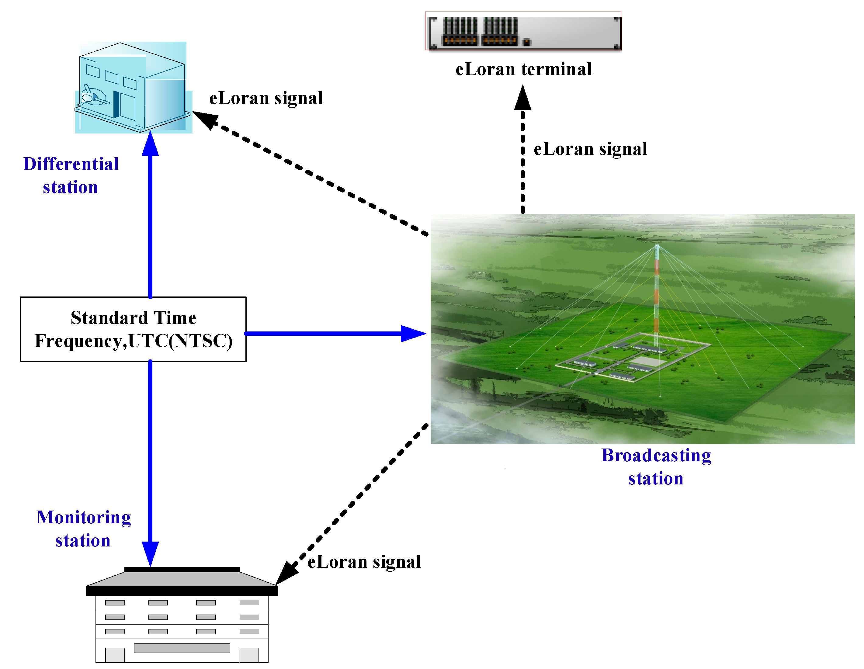
2.1. Principle of eLoran Time Service System

The principle of the eLoran system evolved from the Loran-C system; eLoran is an internationally standardized positioning, navigation, and timing (PNT) service system with the advantages of long range, good stability, high reliability, and strong anti-interference capability. The timing service can usually achieve a ground-wave timing accuracy of better than 1 μs, and a timing accuracy of better than 100 ns can be realized by using differential technology [14].
The structural components of the eLoran system generally include a broadcasting station, monitoring station, and differential enhancement station as shown in Figure 1. Among them, the broadcasting station adopts solid-state transmitter technology and data chain technology to realize high-precision time signal broadcasting; the monitoring station is set up to ensure the reliability and accuracy of time broadcasting; and the differential enhancement station is set up to improve the accuracy of time broadcasting.
All broadcasting stations are time-synchronized, and trace back to the Chinese standard time UTC (NTSC) kept by the National Timing Center.
The timekeeping system at the eLoran monitoring station is traceable to UTC (NTSC), an eLoran signal belongs to the long-wave band, and the propagation performance is stable; by comparing the time difference between the output time signal of the monitoring receiver and the time signal of UTC (NTSC), you can judge the working condition of the broadcasting station and make an early warning.
The differential enhancement station monitors the correction amount of the timing deviation of an eLoran timing signal in a certain area and broadcasts it to the user by the system, and the user obtains high-precision timing service after deducting the correction amount of timing deviation.

2.2. Near-Field Monitoring Station

According to the wave propagation characteristics of the eLoran, the BPL monitoring system is constructed to match the near-field and far-field monitoring, so as to continuously monitor the integrity and accuracy of the BPL timing signal in the monitoring coverage area, and to ensure that the BPL timing signal can be used, usable, and good.
The structural components of the eLoran monitoring system are mainly composed of three parts: the near-field monitoring station, far-field monitoring station, and data processing center.
The near-field monitoring station is located at the BPL time service station, which is mainly used to monitor the accuracy of the broadcasting control of the time service station, collect the BPL signal from the root of the transmitting antenna through the current transformer, and demodulate the time code information and 1PPS (plus per second) signal contained in the BPL signal through the BPL monitoring receiver. The structure of the near-field monitoring station is shown in Figure 2, which is mainly composed of four parts: the data acquisition equipment, time interval counter, time-frequency keeping equipment, and enhanced Roland timing terminal.
The time-frequency keeping unit consists of a cesium atomic clock, 5071A (accuracy ±1.0 × 10⁻¹², stability ≤ 1.2 × 10⁻¹¹ for 1 s averaging time, long-term stability ≤ 5.0 × 10⁻¹⁴ for 5-day averaging time), and a fiber optic traceability system, which provides standard 10 MHz and 1PPS signals, and traces back to the Chinese standard time UTC (NTSC) kept by the National Timing Center through optical fiber. The 1PPS signal output from the BPL monitoring receiver is compared with the 1PPS output from the time-frequency keeping unit through the time interval counter (model number SR620, 25ps single-shot time resolution), and the control accuracy of the BPL signals can be analyzed through the analysis of the comparison data [14,15,16,17,18].

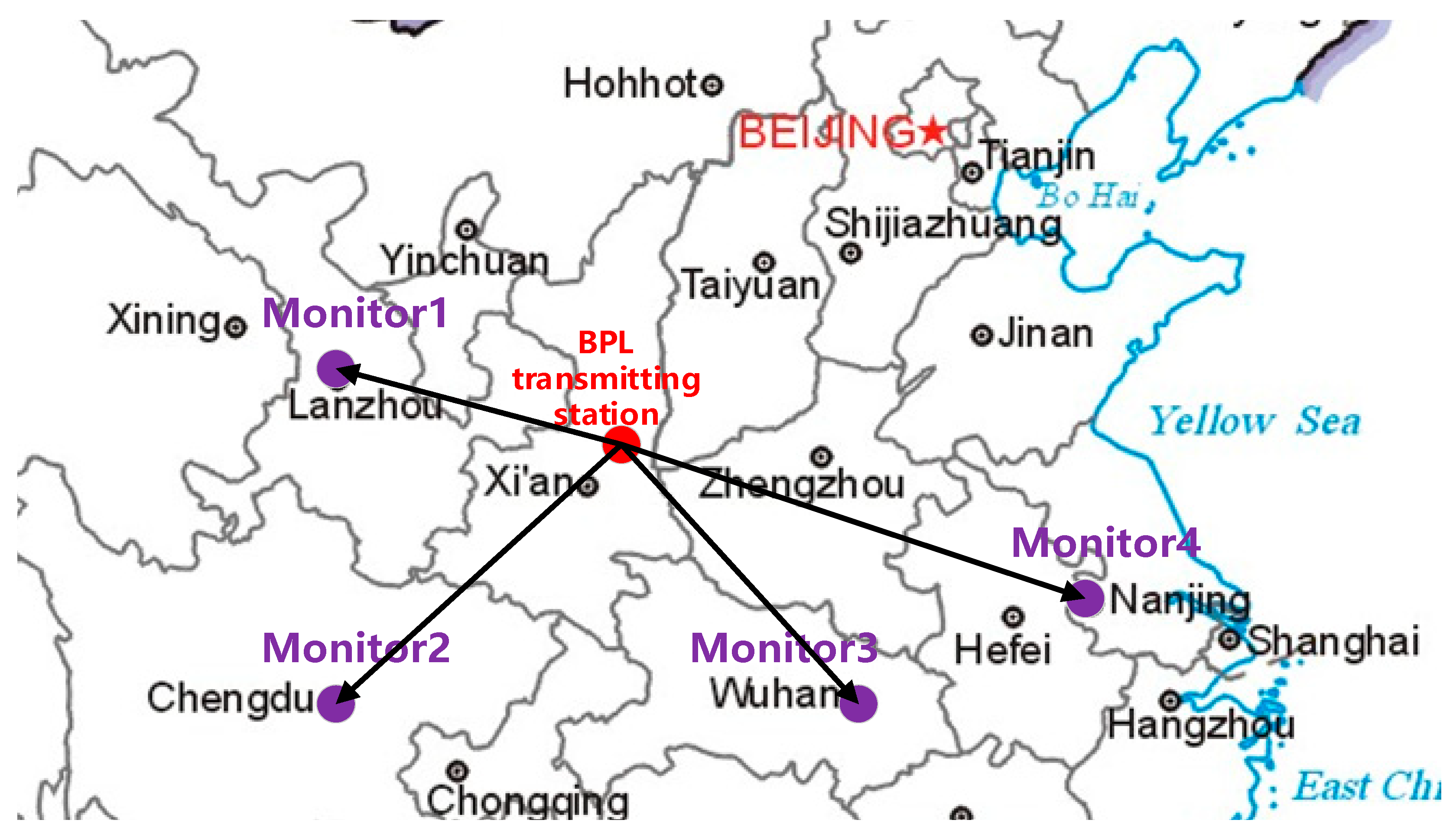
2.3. Far-Field Monitoring Station

The propagation characteristics of eLoran signals have large path variability, so the distance from the BPL time service station and the difference in geographical direction will cause the difference in the propagation characteristics of timing signals, including the propagation delay, field strength, signal-to-noise ratio changes, etc. Therefore, this design mainly considers the construction of four monitoring stations with different distances from the BPL time service station. Therefore, this design mainly considers the construction of four monitoring stations with different distances in four different directions of the BPL station to monitor the quality of the BPL signal in real time, and the monitoring data are transmitted to the BPL monitoring data processing center.
The overall design scheme of the far-field monitoring station is shown in Figure 3, and the equipment components of the far-field monitoring station mainly include a BPL monitoring receiver, time and frequency traceability keeping unit, time interval counter, and data processing and transmission platform.
Its main working principle:
  • The time-frequency traceability keeping unit realizes time traceability to China standard time UTC (NTSC) through BDS (BeiDou Navigation Satellite System) common-view comparison, and provides a high-precision 1PPS reference signal (measurement reference), a 10 MHz frequency standard signal, and UTC time code information;
  • The BPL monitoring receiver outputs a 1PPS timing signal, a 10MHz frequency calibration signal, and time code data information by receiving a BPL signal;
  • The time interval counter receives the time difference data by measuring the 1PPS and reference 1PPS output from the BPL monitoring receiver, and receives the time code monitoring comparison data by comparing the time code information;
  • The monitoring receiver transmits the time difference data and time code data obtained from the measurement comparison to the monitoring data processing center through the network.

2.4. Data Processing Center

The BPL monitoring data processing center realizes a comprehensive processing and analysis and evaluation of monitoring data gathered by each monitoring station, evaluates and assesses the performance of the BPL time service system and the integrity and availability of current BPL signals, and realizes the functions of an abnormal alarm for time difference, abnormal alarm for time code, and abnormal alarm for power.

3. Near-Field Monitoring Station Performance Analysis

The near-field monitoring station is located in the BPL time service station, which mainly monitors the precision of transmission control. The near-field monitoring station transmission control accuracy test uses the BPL timing monitoring receiver to collect the current transformer sampling signal at the root of the transmit antenna, and conducts the timing output comparison test to eliminate the error introduced by the receiver, which is the timing transmission control accuracy. However, since it is not easy to separate the receiver error, the time difference between the 1PPS signal output from the monitoring receiver and the standard 1PPS signal is measured directly and analyzed and calculated to obtain the timing and transmission control accuracy [19,20,21,22,23,24,25].
The 1PPS signal output from the time-frequency reference unit is the reference, and the 1PPS signal output from the BPL timing monitoring receiver is the measured signal; the time difference measurement data output from the time interval counter measurement is used for the calculation of the transmission control accuracy.

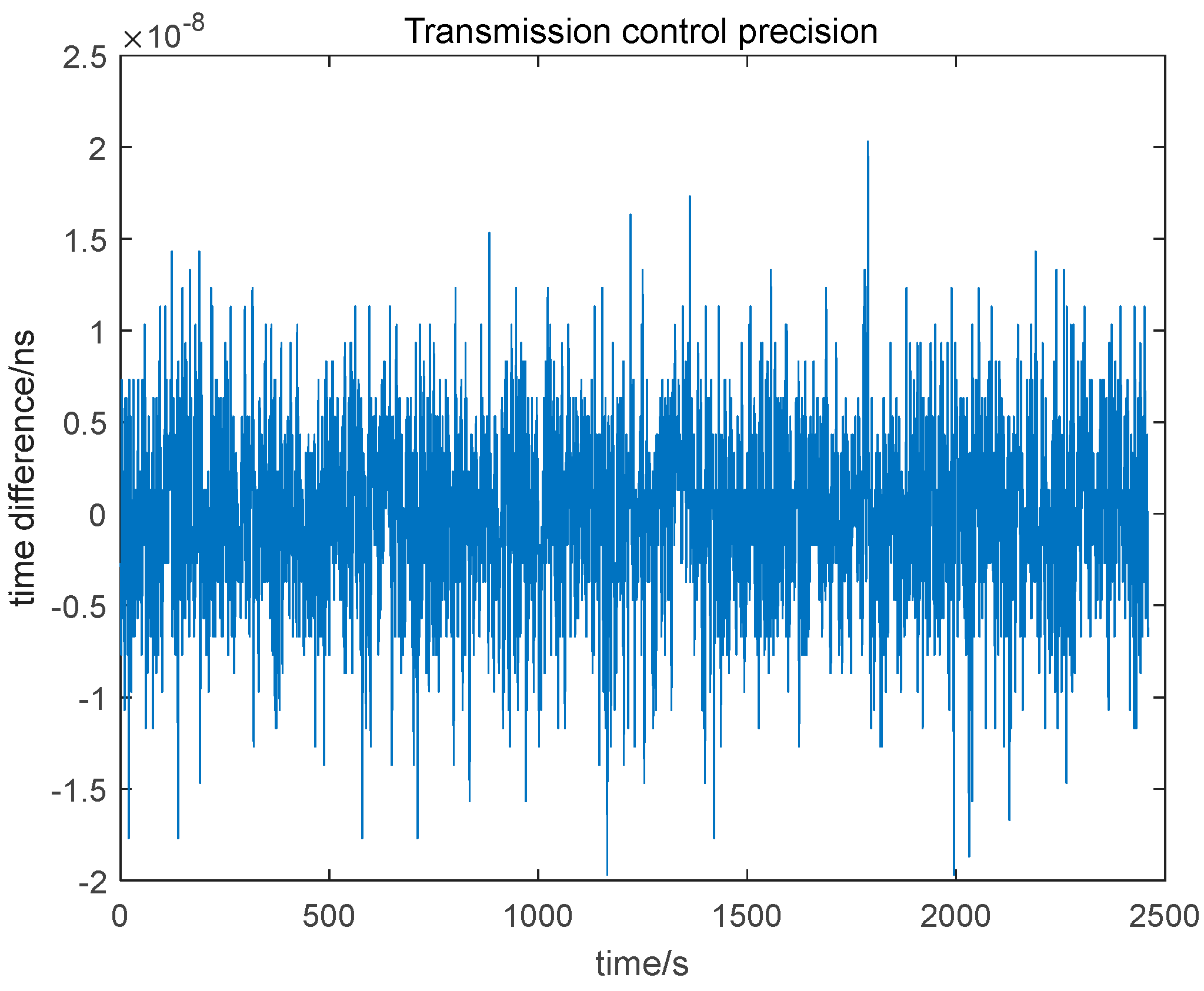
3.1. Transmission Control Precision Calculation Method

The transmission control accuracy is expressed by the standard deviation of the measured 1PPS time difference, once data are measured per second, for i sets of data. It is represented by Formula (1).
σ = 1 i T X i T X 2 i
In the formula,
σ is the transmission control accuracy in ns;
TXi is the time difference data obtained from the ith measurement of the time interval counter, in ns;
TX is the mean value of the time difference data in ns.

3.2. Transmission Control Precision Data Analysis

According to the test method of transmission control accuracy of the near-field monitoring station, the test was carried out in the BPL time service system. After the calculation and analysis of the test data for a long time, as shown in Figure 4, the standard deviation of the time difference between the 1PPS signal output by the monitoring receiver and the UTC (NTSC) standard 1PPS signal is 6.24 ns, which is less than 30 ns. It meets the requirement of the transmission control precision index of the eLoran system.

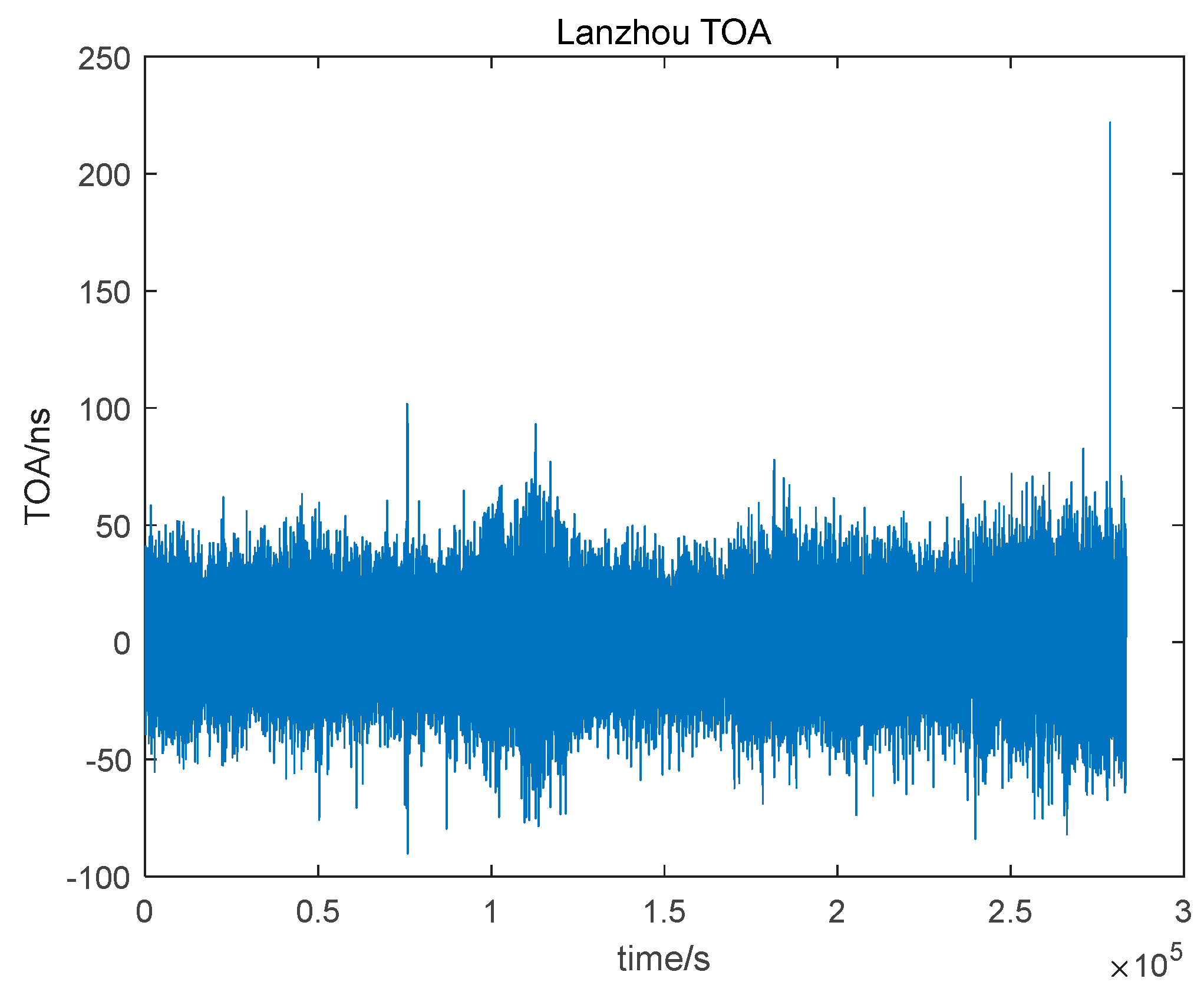
4. Far-Field Monitoring Station Performance Analysis

The four far-field monitoring stations of the BPL monitoring system are located in the coverage area of the BPL ground-wave signals, and suitable locations are selected in different directions for layout and construction. According to the experimental test, the layout of the far-field monitoring stations is mainly set up in four different directions of the BPL station, and the distance of the four far-field monitoring stations from the BPL station varies from 500 to 900 km. The far-field monitoring stations are mainly used to monitor the changes in the time-of-arrival (TOA) value, and to analyze the performance of the transmitter–radiator through these worthwhile changes. The coordinate information and distribution map of the far-field monitoring stations are shown in Table 1 and Figure 5 [19,26,27,28,29,30].
The difference between the 1PPS output from the BPL monitoring receiver and the 1PPS output from the time-traceable keeping unit, which is subtracted from the propagation time and the receiver delay, is the TOA value, and the performance of the BPL signal is judged by analyzing the change in the TOA value and the standard deviation. Figure 6, Figure 7, Figure 8 and Figure 9 show the trend of TOA values for Lanzhou, Chengdu, Wuhan, and Nanjing. Table 2 shows the standard deviation of TOA values of each monitoring station.
From Figure 6, Figure 7, Figure 8 and Figure 9, it can be seen that as the distance increases, the STD value of TOA becomes larger and larger, indicating that the jitter in the TOA value also increases.
The Wuhan station is slightly closer to the BPL than the Chengdu station, but the STD of the TOA value is larger, mainly because the Wuhan station is located in the center of the city of Wuhan, which has a complex electromagnetic environment and a lower signal-to-noise ratio. The Chengdu station is located in the suburb of Chengdu, with a better electromagnetic environment and a higher signal-to-noise ratio. The receiver antenna installation environment is shown in Figure 10.
BPL adopts the eLoran signal system, which belongs to a low frequency and long-wave signal. The increase in TOA jitter is mainly caused by the difference in the propagation path. However, in the same location, the trend of the TOA value is basically the same.

5. Integrity Monitoring Analysis

The BPL signal belongs to low-frequency long-wave signals in the same location where the signal trend is relatively stable, and this paper uses the TOA value to analyze the intactness; based on the TOA in the history of the data for prediction, when the gap between the predicted value and the actual value is too large, it is issued as a warning to the BPL time service.

5.1. Time Difference Prediction Model

The basic idea of time difference prediction is to utilize the existing historical data of the TOA to predict the current TOA value through the prediction model.
In this paper, the Kalman filter prediction model is used; Kalman filtering is an algorithm that uses a series of measurements observed over time, including statistical noise and other inaccuracies, and produces estimates of unknown variables that tend to be more accurate than those based on a single measurement alone, by estimating a joint probability distribution over the variables for each timeframe [31,32,33,34,35].
The Kalman filter consists of two main stages: the prediction stage and the update stage. Theoretical derivations are given in Equations (2)–(11).
1. Prediction Stage
In the prediction stage, the current state estimate and the system model are used to predict the state and error covariance at the next time step.
Predict the next state:
x k | k 1 = A x k 1 | k 1 + B u k
xk|k−1 is the predicted state at time k, xk−1|k−1 is the estimated state at time k−1, A is the state transition matrix, B is the control input matrix, and uk is the control vector.
Predict the error covariance:
P k | k 1 = A P k 1 | k 1 A T + Q
Pk|k−1 is the predicted error covariance, Pk−1|k−1 is the error covariance at time k−1, and Q is the process noise covariance matrix.
2. Update Stage
In the update stage, the predicted state and error covariance are updated using the new measurement.
Compute the Kalman gain:
K k = P k | k 1 H T H P k | k 1 H T + R 1
Kk is the Kalman gain, H is the measurement matrix, and R is the measurement noise covariance matrix.
Update the state estimate:
x k | k = x k | k 1 + K k z k H x k | k 1
zk is the measurement at time k.
Update the error covariance:
P k | k = I K k H P k | k 1
I is the identity matrix.
3. Iteration
For each time step k,
Prediction Stage:
x k | k 1 = x k 1 | k 1
P k | k 1 = P k 1 | k 1 + Q
Update Stage:
K k = P k | k 1 P k | k 1 + R
x k | k = x k | k 1 + K k z k x k | k 1
P k | k = 1 K k P k | k 1
By following these steps, the Kalman filter recursively estimates and predicts the state of one-dimensional time difference data.
4. Parameter setting
For the application scenario in this paper, in the prediction with Kalman filtering, a certain amount of historical data need to be selected for the prediction of the latter data, and the parameter num_pre is the amount of historical data needed for the prediction; in order to determine this parameter, the experiments were performed for num_pre = 1, num_pre = 2, num_pre = 3, num_pre = 5, num_pre = 10, and num_pre = 20, and performing the experiment with the same remainder of the parameters, the root mean square error is 0.0083874, 0.0073235, 0.0073572, 0.0078228, 0.0082398, and 0.0082664, respectively. The root mean square error is smaller when num_pre = 2. Therefore, we choose to take the historical data of the first two moments as a prior for predicting the time difference data of the latter moment.
The ideal value of the time difference is 0, so the initial state is set to 0.
Process noise covariance Q is set to 0.01.
Measurement noise covariance R is set to 0.1.
Initial error covariance P is set to 1.
Since the next momentary state is not significantly correlated with the previous momentary state, state transition matrix A is set to 1.
Measurement matrix H is set to 1.

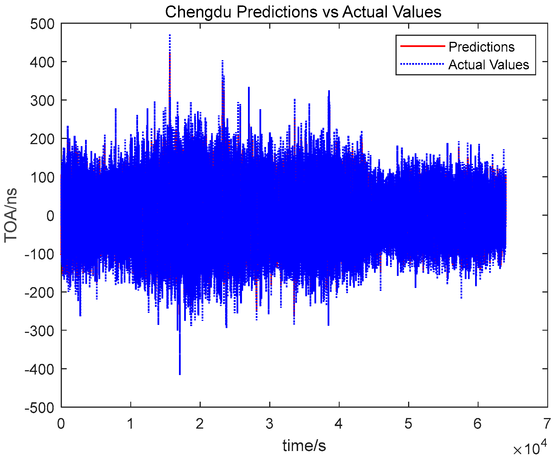
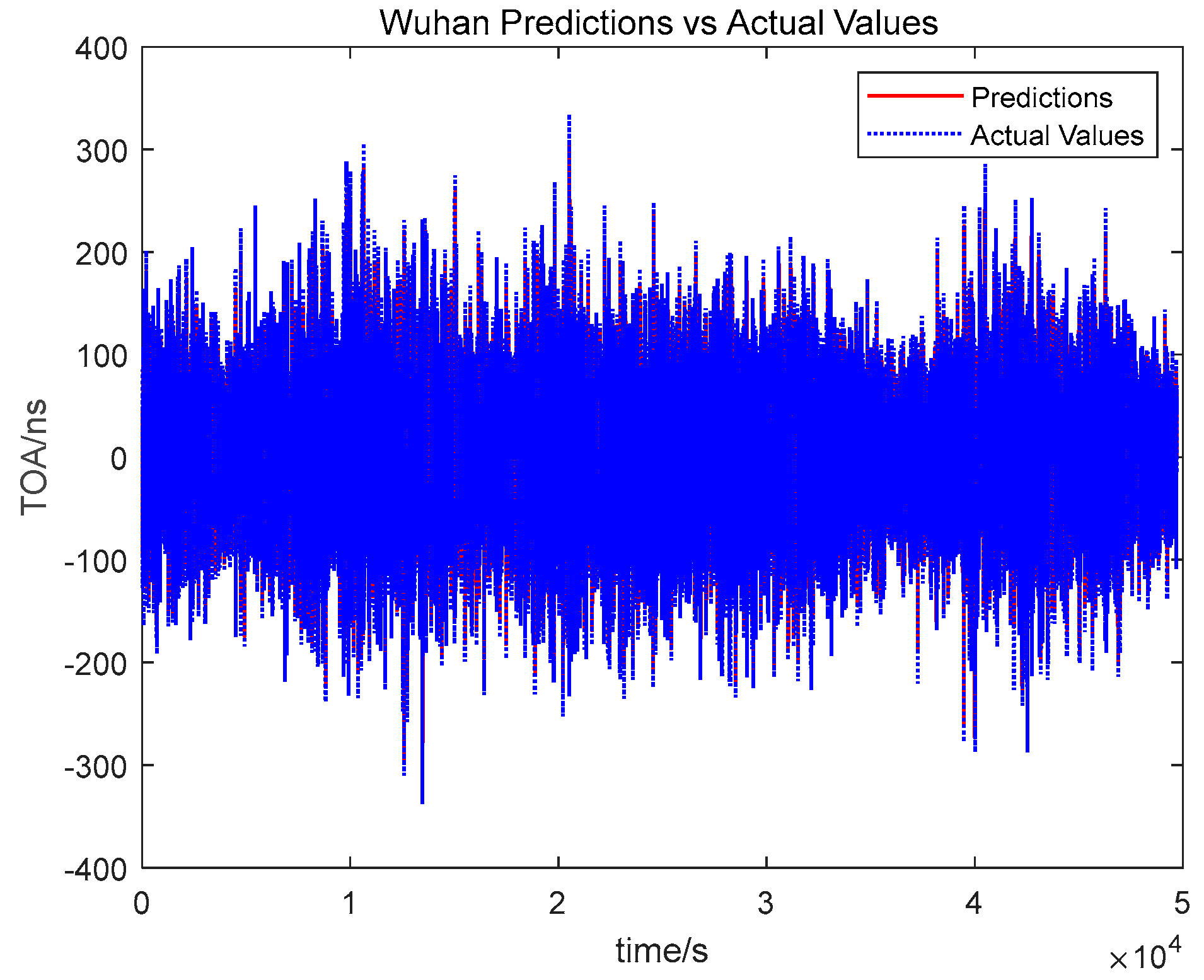
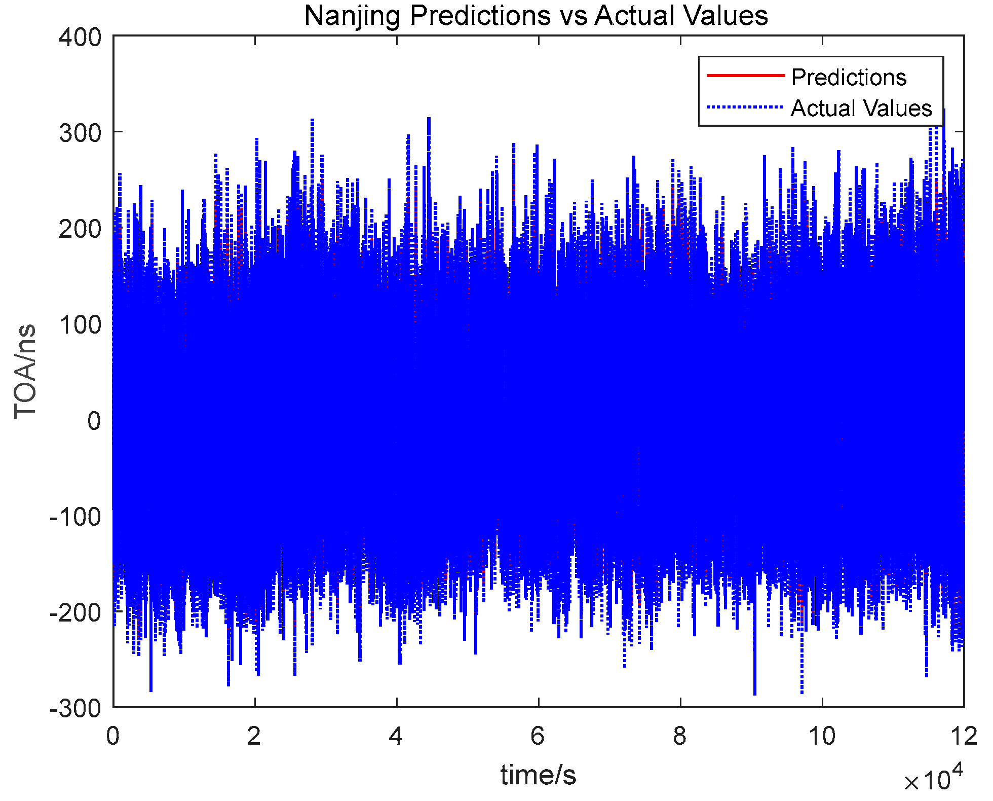
5.2. Predictive Performance Analysis

An important part of integrity monitoring is the prediction of the TOA. The closer the predicted TOA value is to the calculated value, the better. Figure 11, Figure 12, Figure 13 and Figure 14 show the trend of the predicted value and actual value for Lanzhou, Chengdu, Wuhan, and Nanjing. Table 3 shows the standard deviation of TOA values of the predicted value and actual value.
From Table 3, we can see that the STD values of the predicted values and the actual values have a relatively high degree of conformity, and the predicted values can reflect the trend of the actual values, and the predicted values can be used as a basis for judging the integrity of the system.

5.3. Thresholds for Integrity Judgments

The actual value and the predicted value should be very close to each other when there is no fault, and when there is a fault in the time service system or a drastic change in the propagation path, the difference between the two values will become larger than the normal error range, which can be used as the basis for the judgment of fault detection.
Before the integrity judgment, a threshold value needs to be determined as the upper limit of error to measure the system without fault. The threshold value is generally obtained empirically, and in practice, it is generally taken as five times the actual value of the STD value.

6. Conclusions

In this paper, the components of the eLoran system are presented, focusing on the working principle and realization path of the monitoring system. And the performance of the monitoring system is verified on the BPL system.
Kalman filter prediction is introduced into the eLoran monitoring system and the difference between the designed prediction value and the actual value is used to determine the state of the transmitter and broadcasting station. The eLoran monitoring system can monitor the status of the eLoran system to ensure the quality of its time service.
Due to the weak correlation between the next moment value of the time difference data and the previous moment data, the prediction can be utilized with less historical data, resulting in a large error between the predicted value and the actual value. The next step is for the authors to try to accumulate more time difference data and to analyze the possibility of applying machine learning to the prediction of the time difference data in order to provide a better monitoring service.

Author Contributions

Conceptualization, C.Y. and S.L.; investigation, C.Y.; resources, S.L.; data curation, X.G. and Z.H.; writing—review and editing, C.Y.; funding acquisition, C.Y. All authors have read and agreed to the published version of the manuscript.

Funding

This research was funded by the Youth Innovation Promotion Association, Chinese Academy of Sciences, grant number: 2021409.

Institutional Review Board Statement

Not applicable.

Informed Consent Statement

Not applicable.

Data Availability Statement

The data presented in this study are available on request from the corresponding author. The data are not publicly available due to the eLoran monitoring system still being under construction.

Conflicts of Interest

The authors declare no conflicts of interest.

References

  1. Enhanced Loran (Eloran) Definition Document, Version 0.1. Available online: https://rntfnd.org/wp-content/uploads/eLoran-Definition-Document-0-1-Released.pdf (accessed on 8 May 2024).
  2. Minimum Performance Standards for Marine eLORAN Receiving Equipment Radio Technical Commission for Maritime Services. Available online: https://rtcm.myshopify.com/collections/maritime-navigation-equipment-standards/products/copy-of-differential-gnss-package-both-of-the-current-standards-10402-3-and-10403-3 (accessed on 8 May 2024).
  3. U.S. Coast Guard and the U.S. Coast Guard Auxiliary. Loran-C User Handbook. Available online: https://www.loran.org/otherarchives/1992%20Loran-C%20User%20Handbook%20-%20USCG.pdf (accessed on 8 May 2024).
  4. Lo, S.; Enge, P. Data transmission using LORAN-C. In Proceedings of the International Loran Association 29th Annual Meeting, Washington, DC, USA, 12–15 November 2000. [Google Scholar]
  5. SAE9990; Transmitted Enhanced Loran (eLoran) Signal Standard. SAE International: Warrendale, PA, USA, 2018. Available online: https://www.sae.org/standards/content/sae9990/ (accessed on 19 August 2024).
  6. SAE9990/1; Transmitted Enhanced Loran (eLoran) Signal Standard for Tri-State Pulse Position Modulation. SAE International: Warrendale, PA, USA, 2018. Available online: https://www.sae.org/standards/content/sae9990/1// (accessed on 19 August 2024).
  7. SAE9990/2; Transmitted Enhanced Loran (eLoran) Signal Standard for 9th Pulse Modulation. SAE International: Warrendale, PA, USA, 2018. Available online: https://www.sae.org/standards/content/sae9990/2// (accessed on 19 August 2024).
  8. Offermans, G.W.A.; Helwig, A.W.S. Integrated Navigation System eurofix: Vision, Concept, Design, Implementation & Test. Ph.D. Thesis, Delft University of Technology, Delft, The Netherlands, 2003. [Google Scholar]
  9. Willigen, D.V.; Offermans, G.W.A.; Helwig, A.W.S. EUROFIX: Definition and Current Status. In Proceedings of the IEEE Position Location & Navigation Symposium, Palm Springs, CA, USA, 20–23 April 1996; pp. 101–108. [Google Scholar] [CrossRef]
  10. ITU-R. P.368-9: Ground-Wave Propagation Curves for Frequencies between 10 kHz and 30 MHz. 2007. Available online: https://www.itu.int/rec/R-REC-P.368/en (accessed on 30 September 2020).
  11. Computational Methods of LW Ground-Wave Transmission Channels, F0130, SJ 20839-2002, People’s Republic of China Electronics Industry Standard. Available online: https://et.wanfangdata.com.cn/bz/Standard/Detail?standardId=SJ%2020839-2002 (accessed on 15 May 2024).
  12. EU eLoran Efforts Sharpen While U.S. Requirements Study Continues. Available online: https://insidegnss.com/eu-eloran-efforts-sharpen-while-u-s-requirements-study-continues/ (accessed on 20 April 2019).
  13. Li, S.F.; Wang, Y.L.; Hua, Y.; Xu, Y.L. Research of Loran-C data demodulation and decoding technology. Chin. J. Sci. Instrum. 2012, 33, 1407–1413. [Google Scholar]
  14. Yang, C.; Li, S.; Hu, Z. Analysis of the Development Status of eLoran Time Service System in China. Appl. Sci. 2023, 13, 12703. [Google Scholar] [CrossRef]
  15. Offermans, G.; Bartlett, S.; Schue, C. Providing a Resilient Timing and UTC Service Using eLoran in the United States: Resilient timing using eLoran. Navigation 2017, 64, 339–349. [Google Scholar] [CrossRef]
  16. Yuan, J.; Yan, W.; Li, S.; Hua, Y. Demodulation Method for Loran-C at Low SNR Based on Envelope Correlation–Phase Detection. Sensors 2020, 20, 4535. [Google Scholar] [CrossRef]
  17. Yang, S.H.; Lee, C.B.; Lee, Y.K.; Lee, J.K. Accuracy Improvement Technique for Timing Application of LORAN-C Signal. IEEE Trans. Instrum. Meas. 2011, 60, 2648–2654. [Google Scholar] [CrossRef]
  18. Wang, X.Y.; Zhang, S.F.; Sun, X.W. The Additional Secondary Phase Correction System for AIS Signals. Sensors 2017, 17, 736. [Google Scholar] [CrossRef]
  19. Son, P.W.; Park, S.H.; Seo, K.; Han, Y.; Seo, J. Development of the Korean eLoran testbed and analysis of its expected positioning accuracy. In Proceedings of the 19th IALA Conference, Incheon, Republic of Korea, 27 May–2 June 2018. [Google Scholar]
  20. Lo, S.C.; Peterson, B.B.; Hardy, T.; Enge, P.K. Improving Loran coverage with low power transmitters. J. Navig. 2010, 63, 23–38. [Google Scholar] [CrossRef]
  21. Li, Y.; Hua, Y.; Yan, B.R.; Guo, W. Analysis on Time Variation Analysis of BPL Long Wave Time Service Signal Transmission Delay. J. Astronaut. Metrol. Meas. 2019, 39, 12–16. [Google Scholar]
  22. Rhee, J.H.; Seo, J. eLoran Signal Strength and Atmospheric Noise Simulation over Korea. J. Position. Navig. Timing 2013, 2, 101–108. [Google Scholar] [CrossRef]
  23. Yan, B.; Li, Y.; Guo, W.; Hua, Y. High-Accuracy Positioning Based on Pseudo-Ranges: Integrated Difference and Performance Analysis of the Loran System. Sensors 2020, 20, 4436. [Google Scholar] [CrossRef] [PubMed]
  24. Lo, S.C.; Peterson, B.B.; Enge, P.K.; Swaszek, P. Loran Data Modulation: Extensions and Examples. IEEE Trans. Aerosp. Electron. Syst. 2007, 43, 628–644. [Google Scholar] [CrossRef]
  25. Yan, W.; Zhao, K.; Li, S.; Wang, X.; Hua, Y. Precise Loran-C Signal Acquisition Based on Envelope Delay Correlation Method. Sensors 2020, 20, 2329. [Google Scholar] [CrossRef] [PubMed]
  26. Hu, A.P.; Gong, T. Research Status and Progress on the Enhance Loran-C Navigation Technology. Mod. Navig. 2016, 1, 74–78. [Google Scholar]
  27. Li, Y.; Hua, Y.; Yan, B.R.; Guo, W. Experimental Study on a Modified Method for Propagation Delay of Long Wave Signal. IEEE Antennas Wirel. Propag. Lett. 2019, 18, 1719. [Google Scholar] [CrossRef]
  28. Safár, J.; Lebekwe, K.C.; Williams, P. Accuracy Performance of eLORAN for Maritime Applicaations. Annu. Navig. 2010, 16, 109–121. [Google Scholar]
  29. Li, S.F.; Wang, Y.L.; Hua, Y.; Yuan, J.B. Loran-C Signal Fast Acquisition Method and Its performance Analysis. J. Electron. Inf. Technol. 2013, 35, 2175–2179. [Google Scholar] [CrossRef]
  30. GBT 14379-1993; Generic Specification Loran-C System. The State Bureau of Quality and Technical Supervision; 1993. Available online: https://std.samr.gov.cn/gb/search/gbDetailed?id=Uu8Zes3Ntyg=&mode=p (accessed on 15 May 2024).
  31. Davis, J.A.; Shemar, S.L.; Whibberley, P.B. A Kalman filter UTC (k) prediction and steering algorithm. In Proceedings of the 2011 Joint Conference of the IEEE International Frequency Control and the European Frequency and Time Forum (FCS) Proceedings, San Francisco, CA, USA, 2–5 May 2011; IEEE: Piscataway, NJ, USA, 2011; pp. 1–6. [Google Scholar]
  32. Luzar, M.; Korbicz, J.; Sobolewski, Ł.; Korbitcz, J. Prediction of corrections for the Polish time scale UTC (PL) using artificial neural networks. Bull. Pol. Acad. Sci. Tech. Sci. 2013, 61, 589–594. [Google Scholar] [CrossRef]
  33. Li, X.H.; Wu, H.T.; Gao, H.J.; Bian, Y.J. Clock disciplined method by using Kalman filter. Control Theory Appl. 2003, 20, 551–554. [Google Scholar]
  34. Ren, Y.; Li, X.-H.; Xue, Y.; Dong, R. Application of Kalmen filter for steering UTC(Lab) to UTC. In Proceedings of the 2014 IEEE International Frequency Control Symposium (FCS), Taipei, Taiwan, 19–22 May 2014; pp. 1–3. [Google Scholar] [CrossRef]
  35. Lin, X.; Luo, Z.-C. A new noise covariance matrix estimation method of Kalman filter for satellite clock errors. Acta Phys. Sin. 2015, 64, 080201. [Google Scholar] [CrossRef]
Figure 1. Working principle of eLoran time service system.
Applsci 14 07350 g001
Figure 2. Component structure of near-field monitoring station.
Applsci 14 07350 g002
Figure 3. Component structure of far-field monitoring station.
Applsci 14 07350 g003
Figure 4. Transmission control precision.
Applsci 14 07350 g004
Figure 5. Distribution map of far-field monitoring stations.
Applsci 14 07350 g005
Figure 6. Trend of TOA in Lanzhou.
Applsci 14 07350 g006
Figure 7. Trend of TOA in Chengdu.
Applsci 14 07350 g007
Figure 8. Trend of TOA in Wuhan.
Applsci 14 07350 g008
Figure 9. Trend of TOA in Nanjing.
Applsci 14 07350 g009
Figure 10. Chengdu and Wuhan receiver antenna installation environment diagram.
Applsci 14 07350 g010
Figure 11. Lanzhou comparison chart of predicted value and actual value.
Applsci 14 07350 g011
Figure 12. Chengdu comparison chart of predicted value and actual value.
Applsci 14 07350 g012
Figure 13. Wuhan comparison chart of predicted value and actual value.
Applsci 14 07350 g013
Figure 14. Nanjing comparison chart of predicted value and actual value.
Applsci 14 07350 g014
Table 1. Coordinates of far-field monitoring stations.
Serial NumberLocationDistance from BPL
1Lanzhou527 km
2Chengdu700 km
3Wuhan675 km
4Nanjing861 km
Table 2. Standard deviation of TOA value.
Serial NumberLocationDistance from BPLSTD of TOA
1Lanzhou527 km16.2 ns
2Chengdu700 km65.4 ns
3Wuhan675 km66.6 ns
4Nanjing861 km70.1 ns
Table 3. Comparison chart of predicted TOA and actual TOA.
Serial NumberLocationSTD of Actual TOASTD of Predicted TOA
1Lanzhou16.2 ns14.5 ns
2Chengdu65.4 ns54.7 ns
3Wuhan66.6 ns61.8 ns
4Nanjing70.1 ns58.2 ns
Disclaimer/Publisher’s Note: The statements, opinions and data contained in all publications are solely those of the individual author(s) and contributor(s) and not of MDPI and/or the editor(s). MDPI and/or the editor(s) disclaim responsibility for any injury to people or property resulting from any ideas, methods, instructions or products referred to in the content.

