Abstract
Stage-built long-span bridges deform with temperature, affecting alignment to design needs. In this paper, a model for predicting temperature time series is proposed, which can predict temperatures in engineering practice and utilize the predicted results to adjust the elevation of stage construction. The model employs convolutional neural networks (CNNs) for initial feature extraction, followed by bidirectional long short-term memory (BiLSTM) layers to capture temporal dependencies. An attention mechanism is applied to the LSTM output, enhancing the model’s ability to focus on the most relevant parts of the sequence. The Crested Porcupine Optimizer (CPO) is used to fine-tune parameters like the number of LSTM units, dropout rate, and learning rate. The experiments on the measured temperature data of an under-construction cable-stayed bridge are conducted to validate our model. The results indicate that our model outperforms the other five models in comparison, with all the R2 values exceeding 0.97. The average of the mean absolute error (MAE) on the 30 measure points is 0.19095, and the average of the root mean square error (RMSE) is 0.28283. Furthermore, the model’s low sensitivity to data makes it adaptable and effective for predicting temperatures and adjusting the elevation in large-span bridge construction.
1. Introduction
Temperature changes can lead to the expansion and contraction of materials, resulting in the deformation of engineering structures. Particularly in materials such as concrete and steel, there are noticeable changes in the shape and dimensions of structures. Large-span complex bridge structures like cable-stayed bridges and suspension bridges cannot ignore the thermal effects such as strain and deflection induced by temperature [1,2]. Lei et al.’s research [3] showed that the tensile stress caused by lateral temperature gradients is significant and cannot be ignored in structural design. In the construction control of large-span concrete cable-stayed bridges, there are quite a few parameters affecting their control precision, with temperature changes having the greatest impact on bridge elevations. In the research by Innocenzi et al. [4], it was pointed out that temperature variations affect the dynamic testing results of newly constructed cable-stayed steel–concrete bridges. Ling et al. [5] found that the longitudinal displacement of the bridge increases with the rise in temperature throughout the day, indicating that temperature variations cause structural responses. Cao et al.’s research [6] indicates that temperature variations have a significant impact on bridge structures, including causing thermal expansion or the contraction of materials, temperature lags, and gradient changes. These factors may lead to displacement and deformation of the bridge, and they can even affect the stability and safety of the bridge. Liu et al. [7] employed a numerical analysis method based on measured temperature fields to study the effect of temperature on the elevation of the main beam. Meanwhile, under the influence of temperature, the main girder of a cable-stayed bridge will exhibit significant deflection, so timely temperature prediction can better assess the health condition of the bridge. Yue et al. [8] provided comparative values for bridge assessment by establishing a correlation model between temperature and temperature-induced deflection. The studies mentioned above calculated the effects of temperature on bridge deformation based on the measured temperature data and could not guide the temperature corrections for construction stage elevations in advance. Therefore, using a more accurate method to predict short-term temperature is of great practical value.
In the early days, people employed models such as the Autoregressive Integrated Moving Average (ARIMA) to forecast and model time series data [9]. In recent years, with the development of machine learning technology, more and more researchers have been engaged in the study of temperature prediction models, which essentially involve time series prediction. Wang K et al. [10] established a model for predicting the vertical and lateral temperature gradients of concrete box girders using a BP neural network optimized by a genetic algorithm, achieving good results. X Shi et al. [11] used support vector machines (SVMs) to predict temperature levels at specific locations. Both models exhibited high temperature prediction accuracy in terms of temperature prediction. However, considering the characteristics of time series—time dependency and periodic trends—traditional machine learning models may have certain advantages on specific datasets, but they may not effectively capture time-related information in trend data. Therefore, models better suited for handling time dependency and dynamic features have emerged, such as recurrent neural networks (RNNs), long short-term memory networks (LSTMs), gated recurrent unit networks (GRUs) [12,13,14,15], etc. These models can better capture the time relatedness and long-term dependencies in time series data.
According to the research, the long short-term memory (LSTM) network outperforms the autoregressive integrated moving average (ARIMA) in terms of performance [16]. Meanwhile, researchers compared the performance of the LSTM model with the SVM on time series data and concluded that LSTM outperformed the SVM in all scenarios [17]. Based on LSTM, Youru Li et al. proposed an LSTM training method incorporating evolutionary attention in 2019. In temperature prediction, this model can achieve competitive predictive performance [18]. Based on LSTM, scholars have further proposed a bidirectional long short-term memory network (BiLSTM). Experimental studies have shown that the BiLSTM model provides better predictions than LSTM models, but the BiLSTM model reaches equilibrium much slower than models based on LSTM [19].
To improve prediction performance, researchers have introduced hybrid models to integrate the strengths of each individual model. The hybrid prediction model combines data preprocessing, optimization algorithms, and ensemble neural networks. Gang Liu [20] proposed an architecture called Attention-based Convolutional Bidirectional Long Short-Term Memory (AC-BiLSTM) to handle sequential data, which achieved good results. This algorithm combines convolutional layers with attention mechanisms, improving the BiLSTM algorithm. The convolutional layer is used to extract information from the initial data, and the attention mechanism is used to give different weights to the output of the BiLSTM hidden layer. Z Wang et al. [21] derived the hyperparameters of the random forest (RF) model through the Bayesian optimization algorithm, enabling accurate assessments of the temperature field for the design, construction, and maintenance of large-span bridges. Zhang K et al. [22] proposed a temperature time series prediction model, which combined the Seasonal-Trend decomposition based on LOESS (STL) [23] decomposition method, Jump-Upward-Shift-and-Trend (JUST) algorithm, and bidirectional long short-term memory (Bi-LSTM) network [24], which integrated the advantages of various methods, eliminating the fluctuation influence of temperature time series and making accurate temperature predictions. It can be seen that the comprehensive use of models to improve prediction model accuracy is evident and also provides effective and reasonable ideas for solving our problems.
To enhance prediction accuracy, researchers have developed hybrid models that leverage the strengths of individual models. The hybrid prediction model incorporates data preprocessing, optimization algorithms, and ensemble neural networks. Gang Liu [20] introduced the Attention-based Convolutional Bidirectional Long Short-Term Memory (AC-BiLSTM) architecture, which effectively processes sequential data by combining convolutional layers with attention mechanisms to enhance the BiLSTM algorithm. Convolutional layers extract information from the initial data, while the attention mechanism assigns different weights to the BiLSTM hidden layer’s output. Z Wang et al. [21] utilized a Bayesian optimization algorithm to fine-tune the hyperparameters of a random forest (RF) model, enabling precise temperature field assessments for the design, construction, and maintenance of large-span bridges. Zhang K et al. [22] proposed a temperature time series prediction model that integrates the Seasonal-Trend decomposition based on LOESS (STL) [23], the Jump-Upward-Shift-and-Trend (JUST) algorithm, and a bidirectional long short-term memory (Bi-LSTM) network. This approach combines the strengths of various methods to reduce the fluctuation in temperature time series and deliver accurate predictions. These comprehensive model strategies significantly improve prediction accuracy and offer effective solutions to our challenges.
This paper proposes a model for bridge temperature prediction, which combines convolutional networks, attention mechanisms, and Bi-LSTM neural networks, as well as uses the Crested Porcupine Optimizer to optimize the parameters of the network. This model has stronger expressive power and generalization ability in temperature prediction tasks, accurately capturing the regularities of temperature changes and being applicable to various complex temperature transformation scenarios. The attention mechanism was initially used for visual image processing and has since been widely applied to sequence data processing and natural language processing (NLP) [23,25,26,27]. In our data, temperatures often exhibit phased different trends. The model with an attention mechanism can dynamically learn the importance of the input data at each time step, thereby improving the performance and generalization ability of the model. We also use the Crested Porcupine Optimizer (CPO) optimization algorithm to optimize the network model parameters, using the number of LSTM units, Dropout Rate, and Learning Rate as optimization parameters, as well as the model’s Loss as the fitness function for iteration to obtain the best parameters. Using the optimized model to predict temperature series can effectively capture the long-term dependencies of the temperature series and generate accurate forecast results.
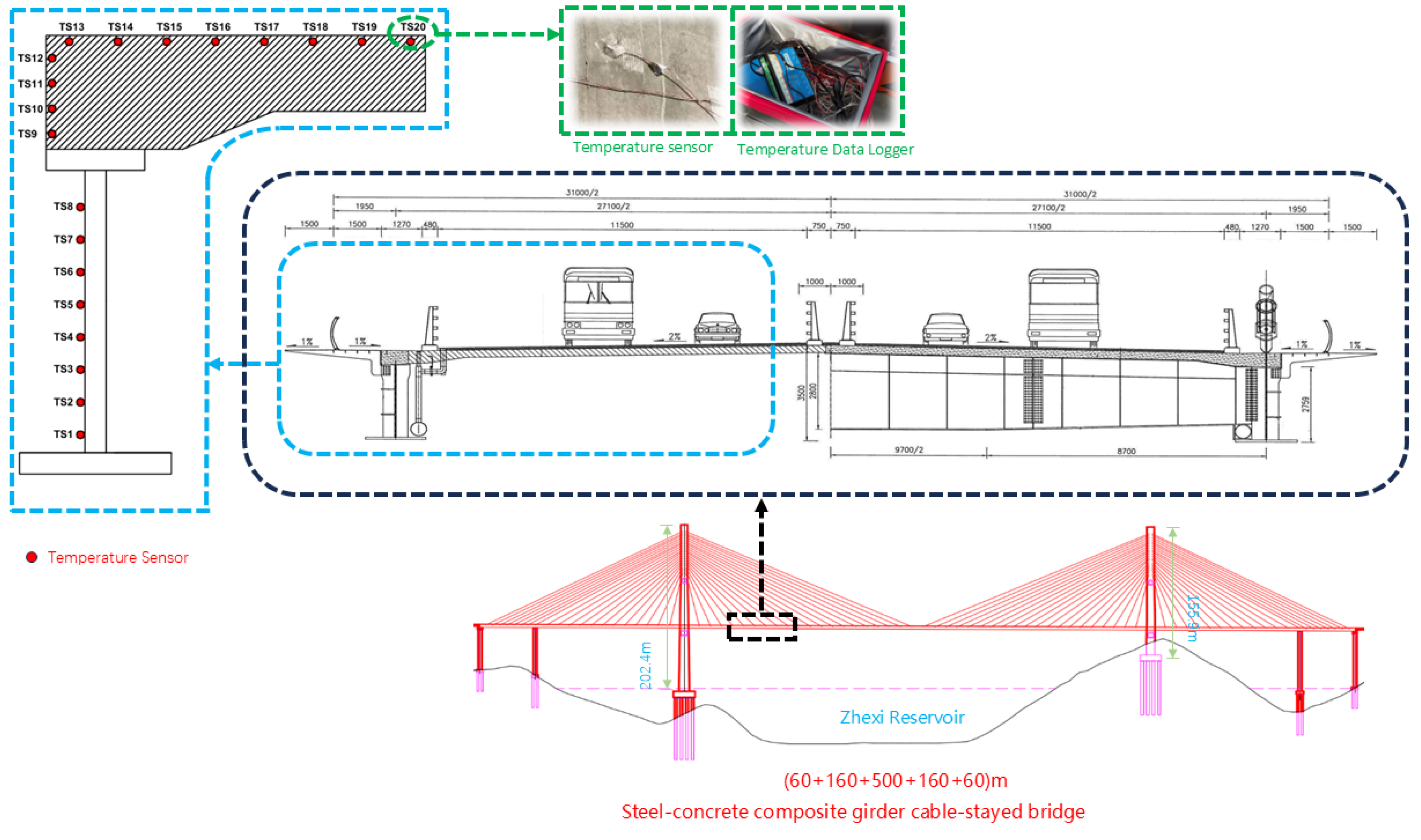
The model can accurately predict the temperature of the main girder, providing important data support for bridge construction and maintenance. Our on-site measurements focus on the vertical temperature distribution of the bridge’s main girder and our predictions target these measurement points as well. The temperature data obtained on-site at the Xuefeng Lake Bridge reflects the vertical temperature distribution of the bridge’s main girder, with the distribution of measurement points shown in Figure 1. This study offers predictive data for analyzing the temperature distribution of the main girder, which can then be used to assess the impact of this temperature distribution on the vertical deformation of the main girder. By considering these impacts during construction, the elevation of the main girder can be adjusted to better meet the design requirements for the bridge’s alignment.
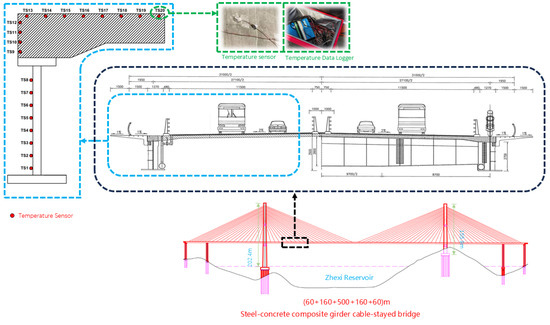
Figure 1.
One of the temperature sensors and data collection devices on the main girder.
The main work of this paper is as follows:
- We proposed a short-term bridge temperature prediction model based on the CPO-CNN-BilSTM-Attention model, which effectively captures the long-term dependence relationship of temperature sequences;
- We used the CPO optimization algorithm to optimize the key parameters of the model to improve the accuracy of the model;
- We used a large amount of real temperature data from Xuefeng Lake Bridge for extensive analysis, proving the generalization ability and stability of the model.
2. Materials and Methods
2.1. Data Materials
This study utilizes data from temperature measurement points on Xuefeng Lake Bridge in Anhua County, Yiyang City, Hunan Province, China. Spanning the Zhexi Reservoir, the bridge measures 1187 m in total length, with a main span of 500 m. It is a double-tower, double-cable-plane, semi-floating system, cable-stayed bridge, and it is a critical project for the Guanxin Expressway as the largest span steel–concrete composite girder cable-stayed bridge in Hunan Province. Temperature sensors installed vertically along the main girder provide surface temperature data from various positions, which we used to train models predicting the girder’s temperature. By analyzing the temperature distribution’s impact on the vertical deformation of the main beams during construction, we can adjust the construction elevation of the main girder. This adjustment ensures that the bridge’s line shape aligns better with design specifications.
The temperature data used in this study were collected from 23 June 2023 to 1 August 2023. Since higher temperatures have a significant impact on bridges, analyzing temperatures in spring, autumn, and winter is less meaningful. Therefore, we chose to use summer temperature data for model training and validation. Each day’s data consists of the temperature readings from 40 measurement points, with temperature recorded once per minute at each point. After preprocessing the data, we obtained 57,600 data points for each measurement point. We randomly selected data from 10 out of 40 temperature measurement points for model training, and the data of the remaining 30 measurement points were used for the model compare experiments. An example of a temperature sensor installation is shown in Figure 1.
Given the small time intervals of the selected data, it is exceptionally well-suited for validating and testing short-term prediction models, effectively meeting the demands of practical engineering applications. However, due to random sensor failures, the data obtained may contain unreasonable values. To address this issue, this study employed the multiple imputation method to handle the erroneous data [28].
2.2. Methods
In this part, we will introduce the methods used in the model proposed in this paper, as well as the conceptual framework of our model. The methods mainly include the attention mechanism, Bi-LSTM, and the CPO optimization algorithm.
2.2.1. Covolutional Neural Network (CNN)
Convolutional neural networks (CNNs) extract local features of input data through convolutional layers, followed by pooling layers to reduce spatial dimensions of features. The CNN structure proposed in this article consists of two One-dimensional convolutional layer (Conv1D), each followed by a One-dimensional max pooling layer (MaxPooling1D) and a Dropout layer. The first Conv1D layer utilizes 64 filters with a size-1 convolutional kernel and ReLU activation function. Subsequently, the MaxPooling1D layer performs pooling with a window size of 2. The second Conv1D layer employs 64 filters with a size-3 convolutional kernel, and it uses ReLU activation.
By utilizing different kernel sizes, the model can capture temporal information at different scales. The first convolutional layer, with a smaller kernel size, helps capture finer-grained features, while the second convolutional layer, with a larger kernel size, captures broader temporal patterns. MaxPooling layers reduce parameters count, mitigating overfitting risk while maintaining feature representativeness. The dropout layers randomly discard outputs of neurons to enhance model generalization. This combination of CNN layers provides rich feature representations for subsequent LSTM layers and attention mechanisms, enhancing the model’s capability to handle series data.
2.2.2. Bidirectional Long Short-Term Memory Model (Bi-LSTM) and Attention
Recurrent Neural Networks (RNNs) [12] are designed to process sequential data, capturing temporal dependencies by passing hidden states across time steps. Long short-term memory (LSTM) [14] is an enhanced RNN architecture that mitigates the gradient problem in sequence processing through the use of forget, input, and output gates. The forget gate discards unnecessary old information, the input gate records relevant new information, and the output gate determines how the current memory state is reflected in the output. These gates enable LSTM to effectively retain long-term information, making it ideal for sequence prediction problems. The structure of an LSTM is depicted in Figure 2.
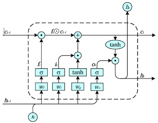
Figure 2.
The structure of LSTM network.
The LSTM network structure consists of the following four steps: updating the forget gate, input gate, cell state, and output gate. Here are the specific four steps introduced below.
and represent the forget gate, input gate, and output gate at time t, respectively. W and b represent the corresponding weight coefficients and biases. represents the hidden state at time . represents the input at time t, and represents the current time step’s cell state. is the candidate value vector. denotes the Sigmoid activation function [14].
Update the Forget Gate:
Update the Input Gate:
Update cell state:
Update the Output Gate:
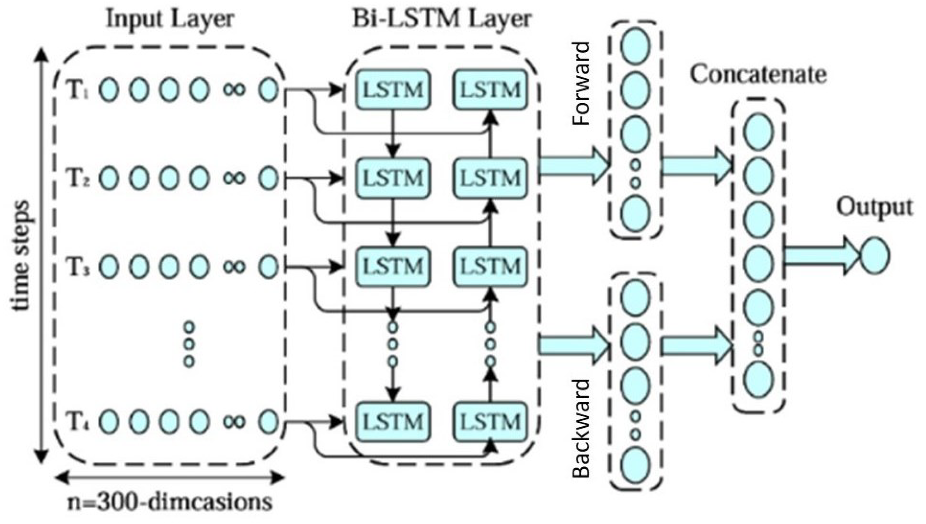
The limitation of LSTM units lies in transferring information only in a single direction, while Bi-LSTM takes into account both forward and backward information, enabling it to capture richer contextual information. The structure of the bidirectional LSTM model is depicted in Figure 3.
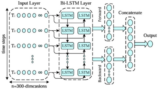
Figure 3.
The structure of Bi-LSTM network.
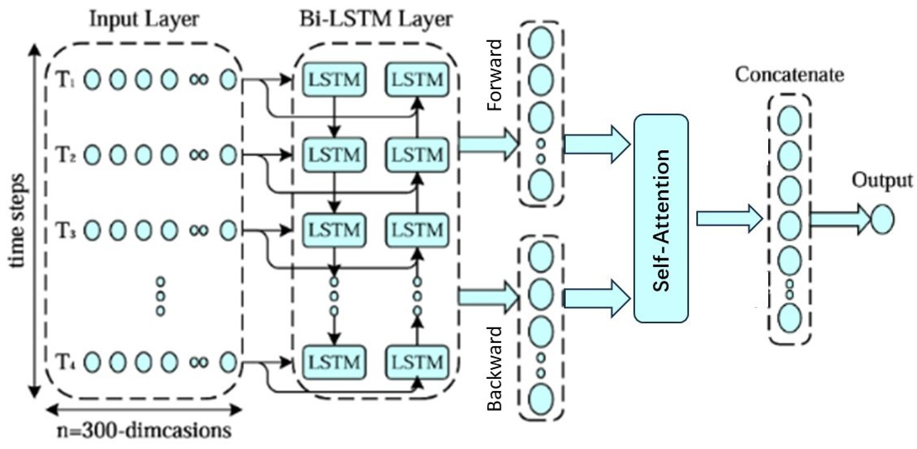
To enhance the generalization capability of the Bi-LSTM, we introduced the self-attention mechanism, which allows the model to dynamically focus on important parts while processing sequences. This combination enables the model to better understand and utilize sequential data, thereby improving its performance and effectiveness.
Self-attention mechanism reduces reliance on external information and is better at capturing internal correlations within data or features. Computing attention involves three stages. In the first stage, the computation of the similarity or correlation between the query and each key (In our implementation of the Attention mechanism, the Key is the output obtained after a Bi-LSTM layer passes through a fully connected layer—the query vector comes from the intermediate representation generated by a convolutional layer) is conducted as follows:
The self-attention mechanism reduces reliance on external information and excels at capturing internal correlations within data or features. Computing attention involves three stages. In the first stage, the similarity or correlation between the query and each key is calculated. In our implementation, the key is derived from the output of a Bi-LSTM layer followed by a fully connected layer. The query vector originates from the intermediate representation generated by a convolutional layer. The computation is performed as follows:
where represents the attention score. are the weight and bias of the attention mechanism. Respectively, refers to the input of the attention mechanism and also represents the hidden states in both directions of output by the Bi-LSTM.
In the second stage, the scores obtained from the first stage are normalized, and the attention scores are transformed using the softmax function, as shown in the following formula:
The final attention value is obtained by the weighted summation of values as shown in the formula:
The Bi-LSTM model with the addition of the Attention mechanism is shown in Figure 4.
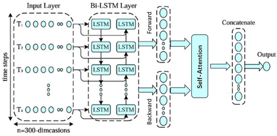
Figure 4.
The Bi-LSTM model with the addition of the Attention mechanism.
2.2.3. Crested Porcupine Optimizer (CPO)
The crested porcupine, a sizable rodent species, is ubiquitous across the globe except for the Antarctic continent. It can be found in a variety of habitats, including forests, arid regions, rocky terrains, and sloping areas. The Crested Porcupine Optimizer (CPO) is an algorithm inspired by the crested porcupine’s defensive tactics, which encompass four levels of aggression: visual, auditory, olfactory, and physical confrontation, escalating in intensity. In the CPO framework, these tactics are mirrored by four separate search domains, each aligning with a specific defensive zone of the porcupine. Zone A represents the initial avoidance behavior, where the porcupine retreats from potential threats. When this initial tactic proves insufficient and predators persist, Zone B is activated, signifying the second line of defense. If the predator remains undeterred, Zone C is engaged, indicating the third level of defense. Finally, if all previous strategies fail, the porcupine resorts to Zone D, its ultimate protective measure, where it resorts to a direct physical confrontation to safeguard itself, potentially neutralizing the threat.
CPO consists of 4 stages:
- Step 1 Population Initialization: Initialize the population by starting the search from an initial set of individuals (candidate solutions); the optimization problem in this paper consists of three dimension (three parameters to optimize: LSTM Unit, Learning Rate, Dropout Rate). The starting point for each dimension is set by random initialization. This is achieved through a formula, which is as follows:where N represents the population size, indicates the ith candidate solution in the search space, and and are the lower and upper boundaries of the search range, respectively. is a vector initialized randomly between 0 and 1. The initial population can be represented as follows:where indicates the jth position of the ith solution, and N represents the number of population size. We only have three network model parameters to optimize, so the dimension is assumed to be 3, meaning that the maximum value for j in is 3.
- Step 2 Cycle Population Reduction (CPR) Technique: The CPR technique operates by periodically reducing the population size while preserving diversity to accelerate convergence. This strategy is analogous to the behavior of Cape porcupines, where not all individuals engage their defense mechanisms—only those that perceive a threat do so. In this method, some Cape porcupines are selectively removed from the population during the optimization process to quicken convergence and later reintroduced to maintain diversity. This helps avoid the risk of becoming trapped in local minima. The mathematical model for cyclic reduction in population size is shown in Equation (12), where T represents the number of cycles, t denotes the function evaluation, is the maximum value of the evaluation function, and is the minimum number of newly generated population individuals.
- Step 3 Exploration Phase: Utilize the first and second defense strategies for population search.
- First Defense MechanismWhen the CP detects a predator, it responds by agitating its feathers. Subsequently, the predator has two options: it can either advance toward the CP, thereby promoting exploration of the vicinity between the predator and the CP to expedite convergence; or it can retreat from the CP, thereby facilitating exploration of more distant areas to identify unexplored territories. This behavior is mathematically modeled using Equation (13):where denotes the best solution of the evaluation function denotes the position of the predator at the time of iteration denotes a normally distributed random value, and is a random value in .
- Second defense mechanismIn this mechanism, the CP makes sounds and threatens the predator. When the predator approaches the CP, the CP’s moans become louder. Mathematically modeling this behavior is achieved in Equation (14):where and are two random integers between , and t is a random number between [29].
- Step 4 Exploitation Phase: Utilize the third and fourth defense strategies for population search.
- Third defense mechanismIn this mechanism, the CP releases a foul odor that permeates its surroundings, thus deterring predators from approaching. The behavior is modeled using Equation (15):where denotes the position of the ith individual at iteration represents the defense factor, denotes a random value between , and controls the search direction. is a random value between , and signifies the odor diffusion factor.
- Fourth defense mechanismThis mechanism is a physical retaliation. When a predator approaches the CP to initiate an attack, the CP responds with physical force. This interaction is modeled as a one-dimensional non-elastic collision, and it is mathematically represented by Equation (16):where denotes the optimal solution obtained, is a random value between is the convergence rate factor, and represents the average force affecting the CP.
The four defense mechanisms of CPO outlined above fall into two distinct categories: exploration and exploitation phases. During the exploration phase, a trade-off between the first and second defense mechanisms is executed when , with and representing two randomly generated numbers between 0 and 1. In the exploitation phase, the third defense mechanism is employed when ; otherwise, the fourth defense mechanism is activated. is a constant ranging from 0 to 1, and it determines the trade-off between the third and fourth defense mechanisms. We present the simplified mathematical formula for updating the CP position as follows:
where , , , , and are generated within the range of 0 to 1, which is subsequently normalized to derive the desired result .
In this study, we will treat the number of LSTM units, dropout rate, and learning rate as optimization parameters, constituting the population to be optimized. The neural network’s loss function will serve as the fitness function for iterative optimization [29,30,31].
2.2.4. CPO-CNN-BiLSTM-Attention Model
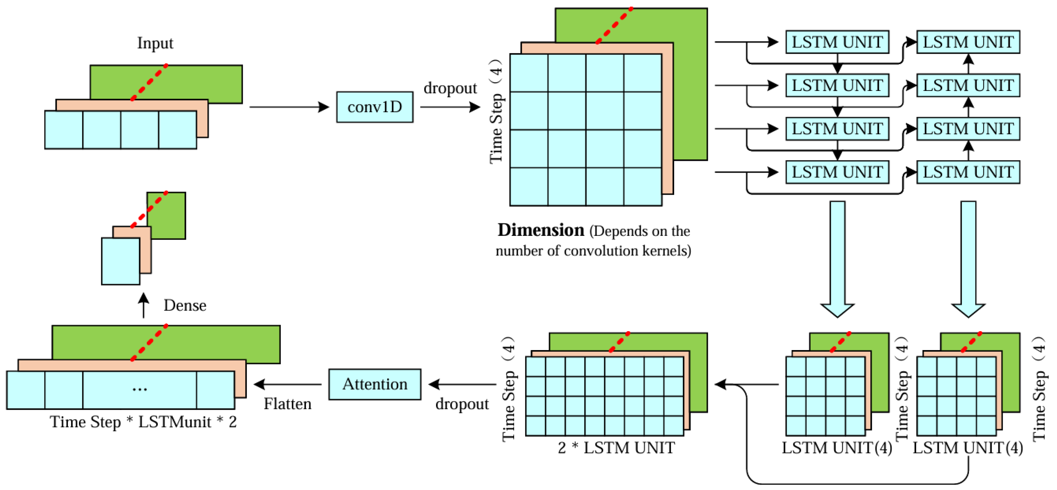
The model proposed in this paper consists of two main components: a deep learning network and an optimization algorithm. The deep learning network comprises a convolutional neural network (CNN), a bidirectional long short-term memory (Bi-LSTM) network, and a self-attention mechanism. After creating a time series with specific time steps, it is fed into the deep learning network. Initially, the input sequence passes through a CNN layer to extract local features. Subsequently, a dropout layer is applied to prevent overfitting. The sequence then enters a bidirectional LSTM layer to capture long-term dependencies within the input sequence and to output the entire sequence. Next, the attention mechanism function is invoked to perform attention-based weighting on the output of the Bi-LSTM layer. Finally, the weighted output is flattened into a one-dimensional vector through a flattening layer, followed by a fully connected layer to produce a linear value.
As shown in Figure 5, the deep learning network consists of a CNN layer, Bi-LSTM, and an attention mechanism for processing the output vector of Bi-LSTM. Firstly, at the input layer, the model takes a three-dimensional tensor with a shape of (batch size, time steps, input dimension). It then proceeds to the convolutional layer for one-dimensional convolution operation, comprising 64 filters, each with a size 1 and ReLU activation. This layer aims to extract local features of the sequence, while a dropout layer is utilized to randomly dropout some neurons during training to prevent overfitting. Secondly, the input sequence is passed to the Bi-LSTM layer, where it undergoes forward and backward learning to capture long-term dependencies within the sequence. The output is then processed by the attention mechanism, which weights the vector to allow the model to focus on crucial parts of the input sequence. Finally, the output is flattened into a one-dimensional vector using a flatten layer and fed into a fully connected layer, resulting in a linear value for prediction.
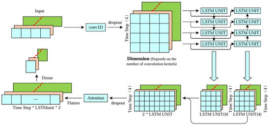
Figure 5.
The neural network component of the temperature prediction network model proposed in this paper.
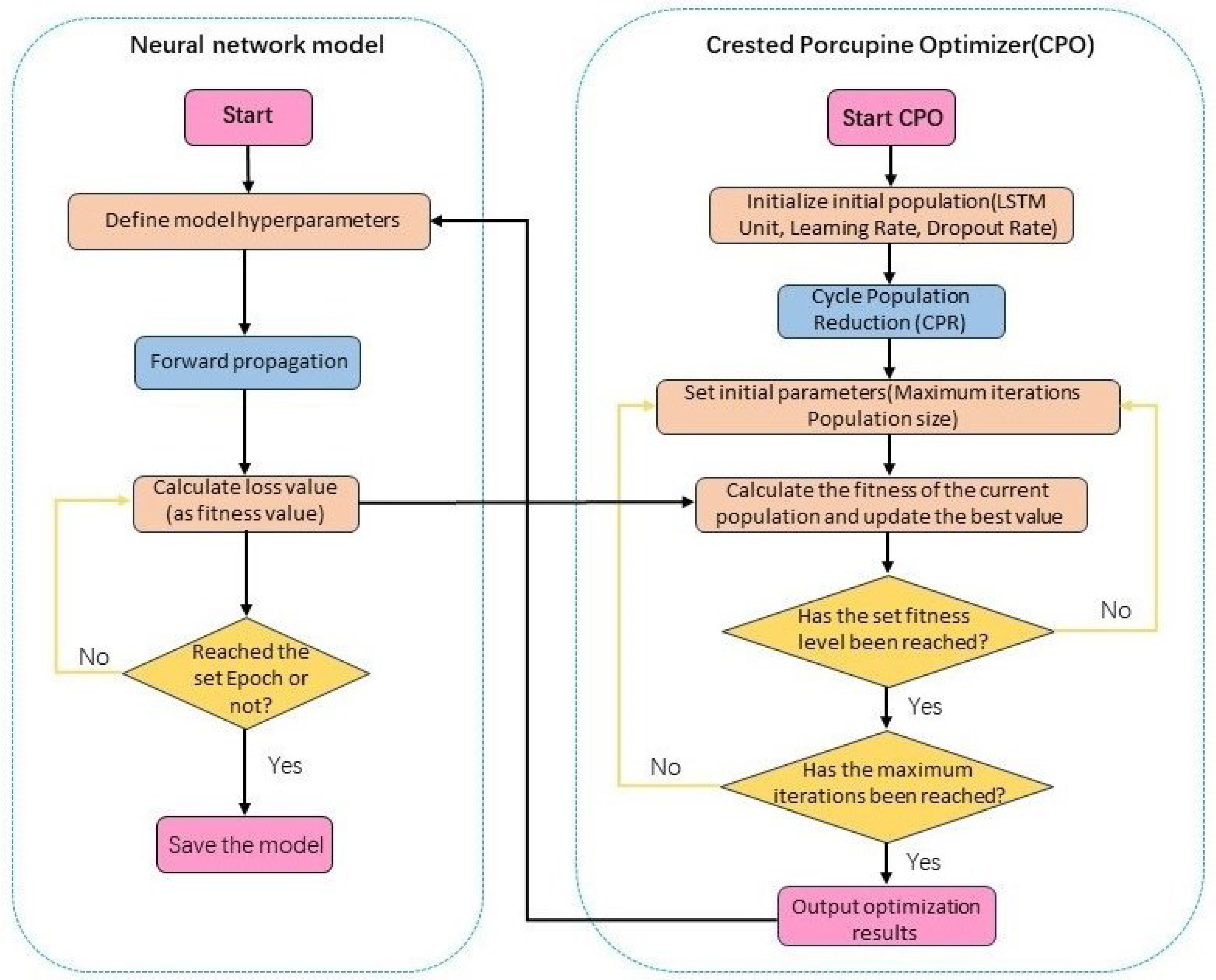
The process of applying the CPO algorithm to optimize the neural network model is illustrated in Figure 6. The optimization algorithm iteratively optimizes the parameters of our network model. We treat the LSTM units, dropout rate, and learning rate of the model as the population for the CPO algorithm. The loss value of the model serves as the fitness function, enabling optimization. In practice, this step is performed first to determine the optimal parameters of the model, thus eliminating the need for laborious manual tuning.
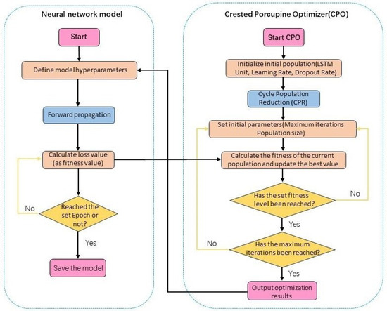
Figure 6.
Flowchart of the CPO optimization algorithm applied to optimize the network model.
3. Results
3.1. Parameters Environment Setup and Loss Function Selection
In our study, the loss function used by the model is the mean squared error (MSE) function, which is expressed as follows:
Among them, represents the true values, represents the predicted values, and n represents the length of the sequence. In the formal experiments, based on our observations, we set the number of epochs for traversing the dataset to 100. This decision was made because, after multiple tests, we noticed an increasing trend in the loss function on the validation set after 100 epochs. For other models, we also chose the corresponding number of epochs based on experimentation. We set the batch size to 32 and the time step to 10. The selection of the remaining three parameters, the number of LSTM units, the learning rate, and the dropout rate, will be optimized and discussed in the optimization module. Meanwhile, Adam optimizer was used in the experiments for its fast convergence speed.
The model proposed in this paper was trained on GeForce RTX3080 using Python 3.7 and Keras version 2.3.1 software and modules.
3.2. Choice of Evaluation Criteria
In order to objectively evaluate the temperature prediction capability of the model proposed in this paper, the root mean square error (), mean absolute error (), and coefficient of determination () were adopted as performance measurement metrics. The expressions for RMSE, MAE, and are as follows:
where is the true value, is the mean value of the time series, is the predicted value, and n is the length of the sequence.
3.3. Experimental Comparison
3.3.1. The Effect of Crested Porcupine Optimizer (CPO)
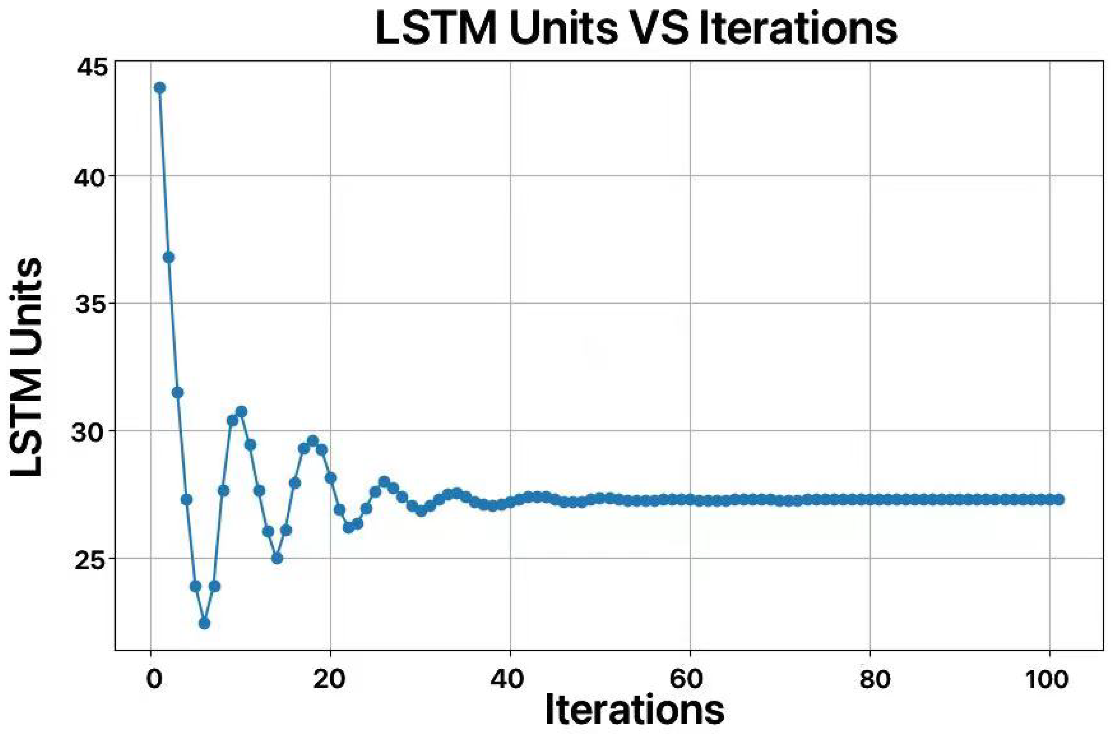
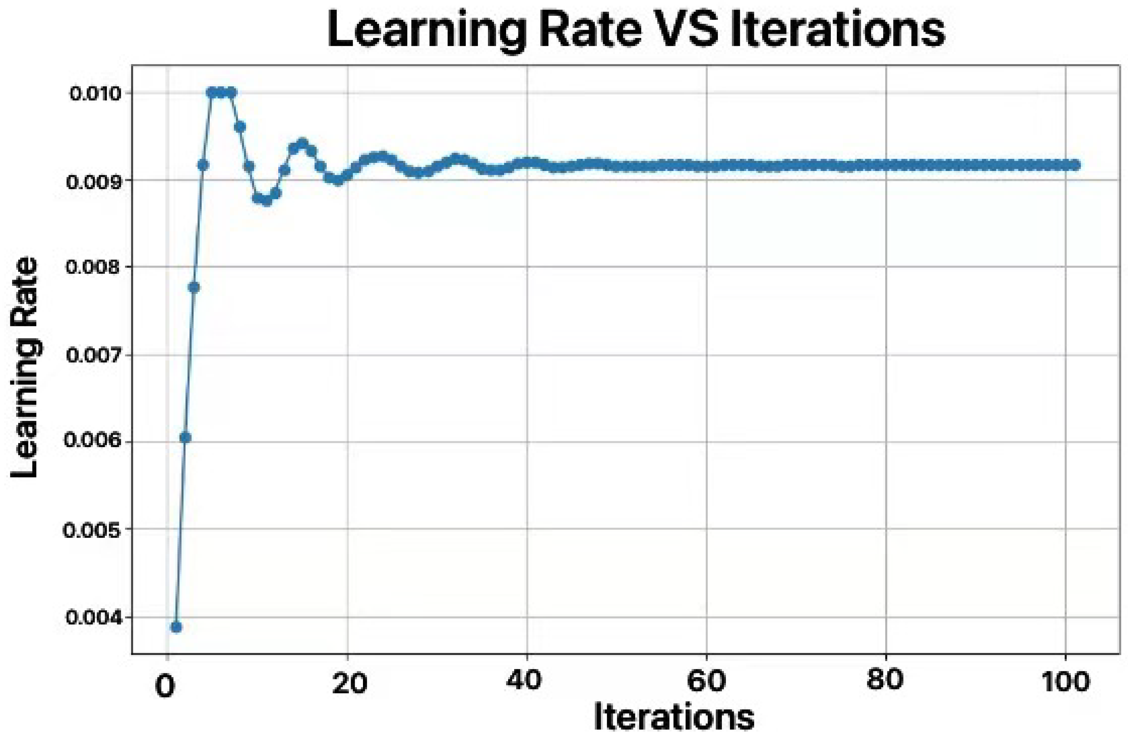
In this study, We utilized the Crested Porcupine Optimizer (CPO) algorithm on the dataset at the temperature measurement point 1 (because the data at point 1 are one of the few datasets that does not require preprocessing, as no dirty data were generated during sensor operation) to optimize the number of LSTM units, learning rate, and dropout rate. We set the number of iterations to 100 to more fully capture the optimization process, but the results showed that the model had already achieved good convergence around the 50th generation. The optimization results are shown in Figure 7 and Figure 8.
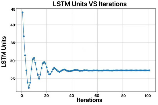
Figure 7.
Curve of optimization for number of LSTM units.
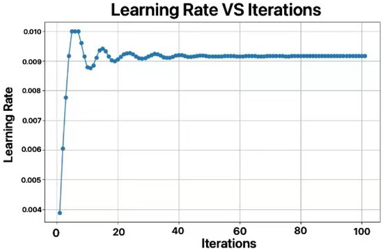
Figure 8.
Curve of optimization for number of learning rate.
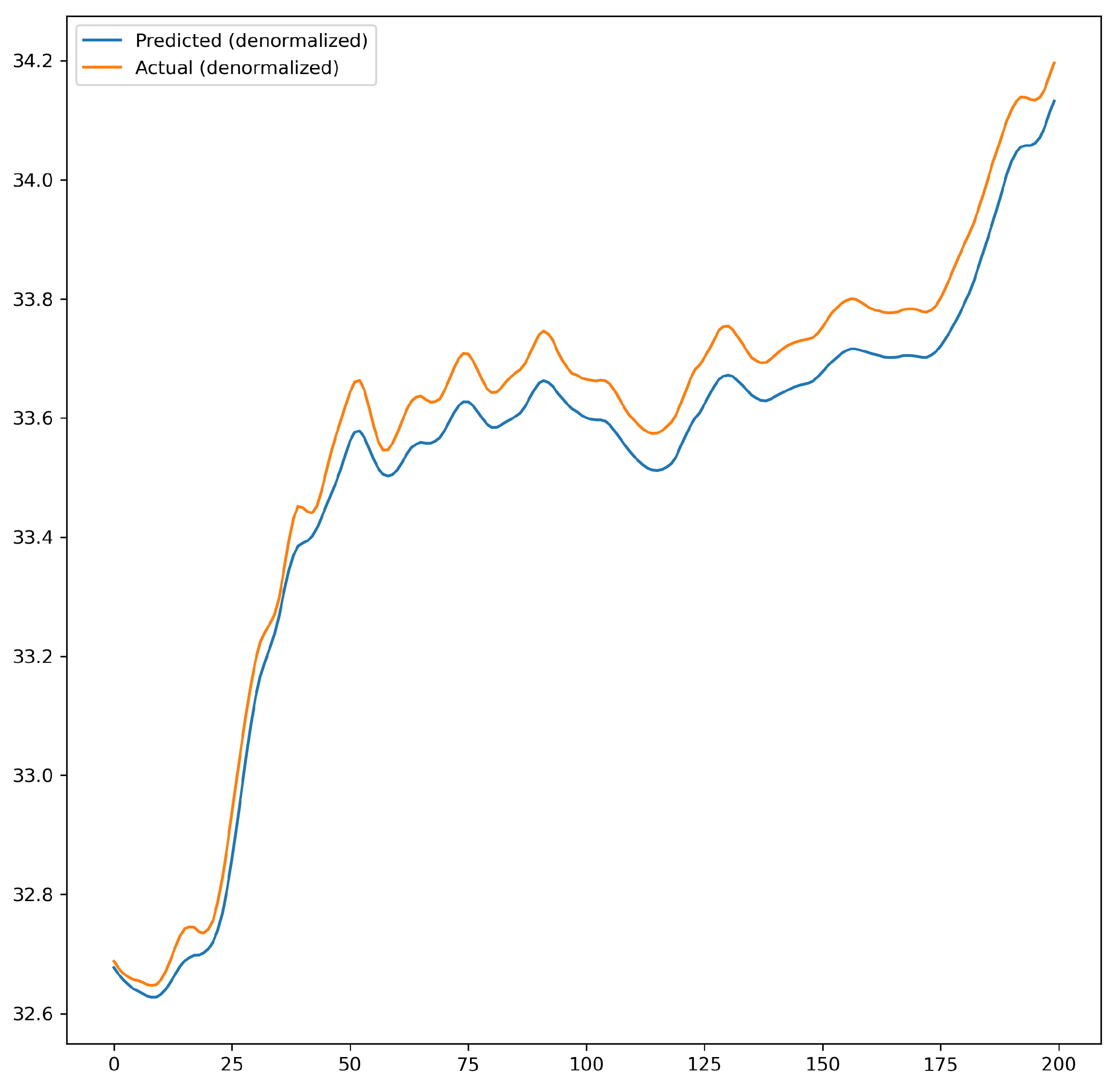
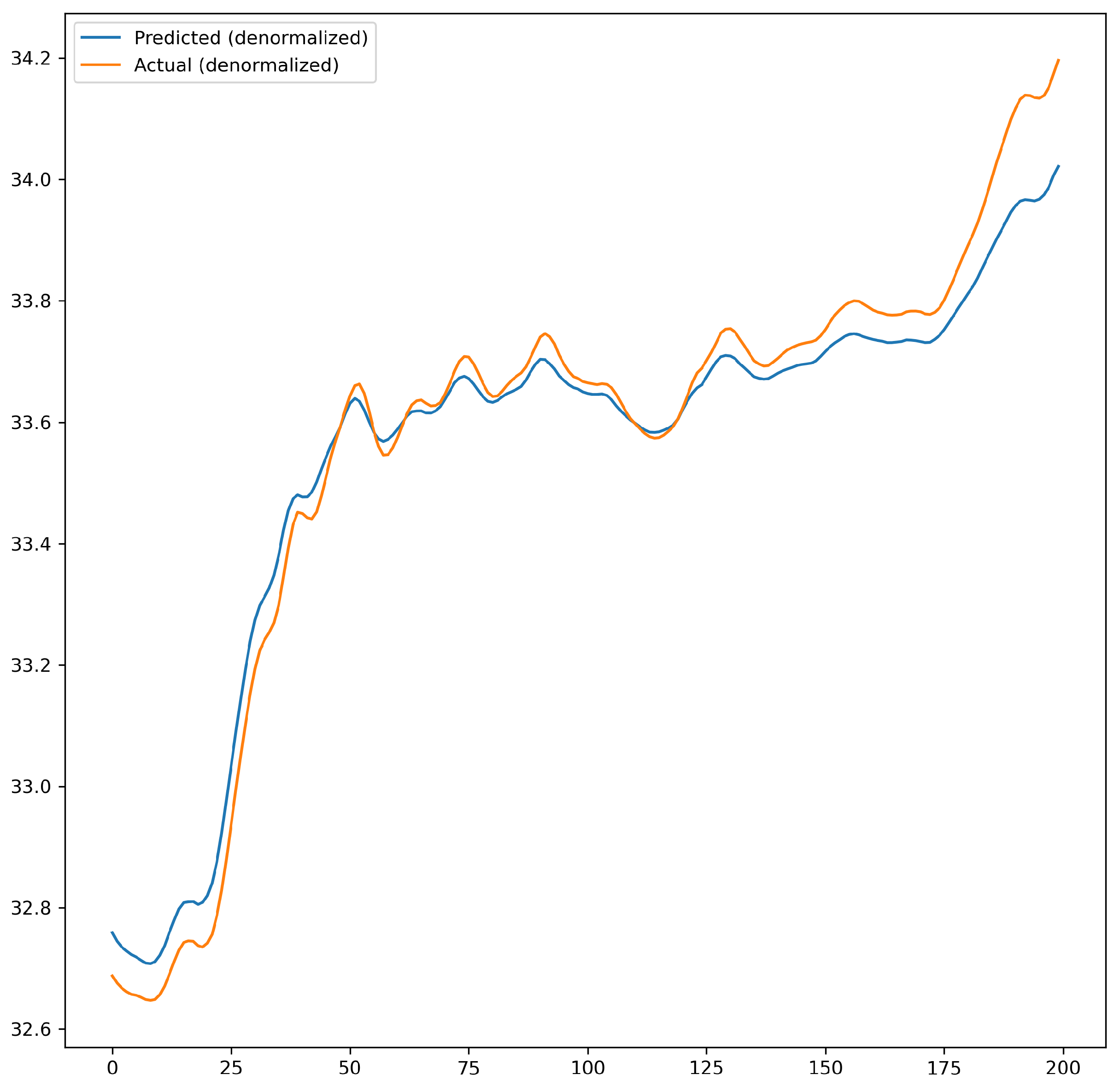
The effect of default parameters and optimized parameters on prediction accuracy was compared. The accuracy was further improved after optimization. As shown in Figure 9 and Figure 10, Figure 9 illustrates the prediction performance of the network model before parameters optimization, while Figure 10 shows the prediction performance after optimization.
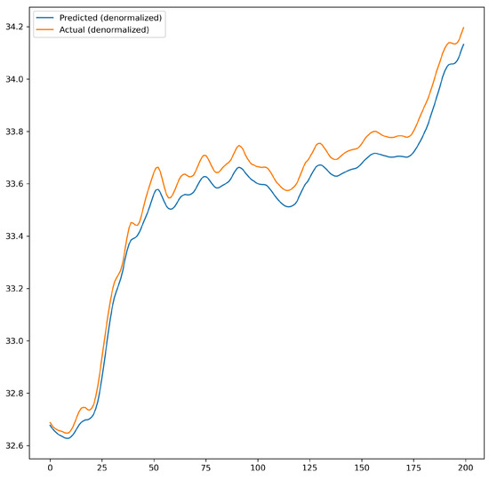
Figure 9.
Prediction performance before optimization of network model parameters.

Figure 10.
Prediction performance after optimization of network model parameters.
After optimization, the number of LSTM units was set to 27, the learning rate to 0.0091, and the dropout rate to 0.3. The commonly used number of LSTM units is 64, but the optimized value of 27 may be due to the periodicity of the weather data, the relatively low complexity of the data, and the modest data volume. Excessive LSTM units could lead to overfitting and increase the computational resource consumption.
We conducted experiments on the models before and after optimization, selecting data from the remaining 30 temperature measurement points at the Xuefeng Lake Bridge for testing. For the ease of presentation, we chose to display the data from the first 15 temperature measurement points using the numbers 1–15 to represent different temperature measurement sites (The complete experimental results are in Table A1 of the Appendix A). The experiment results are shown in Table 1, and it can be observed that the three performance indicators of the optimized model all decreased.

Table 1.
The impact of optimization algorithms on the performance metrics of model prediction results.
In summary, using optimization algorithms for parameters optimization in deep learning networks not only reduces the workload of manual parameters tuning but also enables more extensive testing of different parameters, resulting in more intuitive results.
3.3.2. Model Evaluation
The model evaluation experiment consists of three stages. In the first stage, we conducted ablation experiments on the pre-optimized model to demonstrate the superiority of the optimized model. In the second stage, we compared different types of neural network architectures commonly used for handling time series data using the same test data as in Section 3.3.1. In the third stage, we performed residual analysis to observe the presence of any outliers. Residual analysis was conducted on five randomly selected datasets out of 30.
Firstly, ablation experiments were conducted on the pre-optimized model to demonstrate the superiority of the optimized model. Similarly, we selected data from the first 15 temperature measurement points for display, as shown in Table 2 (The complete experimental results are in Table A2 of the Appendix A). It can be observed from Table 2 that the values of all models are around 0.9, indicating that these models all have certain predictive capabilities. The model proposed in this paper achieved the highest score, while the predictive performance of the remaining models gradually decreased, indicating that optimization of the model was effective.
Secondly, different types of neural network architectures commonly used for handling time series data were compared. Transformer, as an excellent model in natural language processing, also exhibits excellent performance in time series data processing [32]. Meanwhile, GRU, as a variant of LSTM, combines the forget gate and the input gate into a single update gate and also plays a significant role in time series data processing. According to the data in Table 2, both the Transformer and GRU models achieved high levels of performance in temperature prediction. However, the proposed model in this paper achieved even better performance, with scores all above 0.97.
Table 2.
Comparison of between different models.
Table 2.
Comparison of between different models.
| Site | Bi-LSTM | Bi-LSTM-Attention * | Transformer * | GRU * | Our Model |
|---|---|---|---|---|---|
| 1 | 0.87433 | 0.88881 | 0.96347 | 0.96512 | 0.98343 |
| 2 | 0.86245 | 0.89209 | 0.94456 | 0.95924 | 0.98281 |
| 3 | 0.86665 | 0.88945 | 0.95437 | 0.95887 | 0.99022 |
| 4 | 0.86554 | 0.89755 | 0.94864 | 0.96476 | 0.98677 |
| 5 | 0.87221 | 0.88235 | 0.95432 | 0.96543 | 0.98043 |
| 6 | 0.86449 | 0.89112 | 0.96543 | 0.96323 | 0.97864 |
| 7 | 0.87423 | 0.87897 | 0.94552 | 0.94888 | 0.98221 |
| 8 | 0.86999 | 0.88511 | 0.94897 | 0.95732 | 0.97431 |
| 9 | 0.85422 | 0.87553 | 0.94533 | 0.95345 | 0.96943 |
| 10 | 0.86131 | 0.88555 | 0.95342 | 0.94876 | 0.97853 |
| 11 | 0.83511 | 0.82132 | 0.94886 | 0.95443 | 0.97432 |
| 12 | 0.85889 | 0.89181 | 0.96345 | 0.93887 | 0.97866 |
| 13 | 0.86432 | 0.87883 | 0.93995 | 0.96342 | 0.97562 |
| 14 | 0.85764 | 0.86994 | 0.94337 | 0.94543 | 0.97786 |
| 15 | 0.86312 | 0.87443 | 0.95432 | 0.95116 | 0.97434 |
* References [33,34,35] for the experimental model method.
We also conducted experiments to compare MAE and RMSE values. For the RMSE and MAE values of each model in the temperature prediction experiments across 30 temperature measurement points, we still display data from the first 15 measurement points (The complete experimental results are in Table A3 and Table A4 of the Appendix A). Observing Table 3 and Table 4, it is evident that our model has the lowest mean absolute error (MAE) and root mean square error (RMSE) values on average.
Table 3.
Comparison of between different models.
Table 4.
Comparison of between different models.
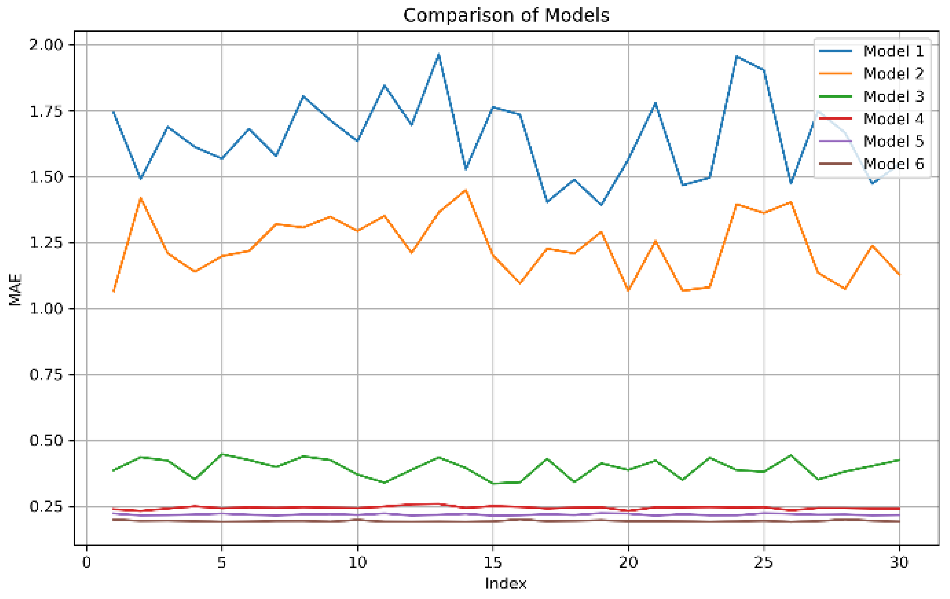
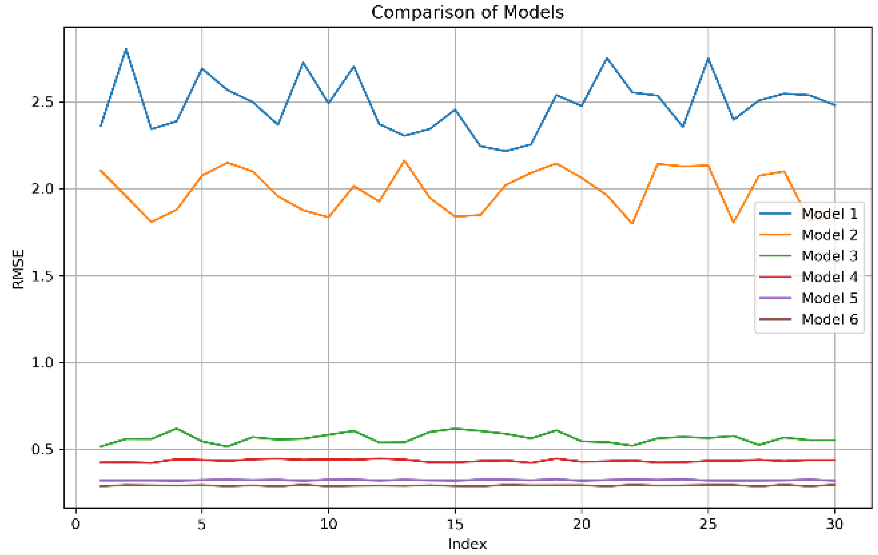
To visualize the MAE and RMSE values, we plotted the MAE and RMSE values to show the trend of changes. The Figure 11 and Figure 12 present the trend of MAE and RMSE for six models after conducting experiments on data from 30 temperature measurement points. The models, labeled as Model 1 to Model 6, are BiLSTM, BiLSTM-Attention, Transformer, GRU, CNN-BiLSTM-Attention, and Our model, respectively. From Figure 11 and Figure 12, it can be observed that Models 1, 2, and 3 exhibited significant fluctuations, while Models 3, 4, 5, and 6 showed much smaller fluctuations. Smaller fluctuation amplitudes indicate that the models are less sensitive to different data, have strong robustness against interference, and are better able to adapt to various data sets. Our model, in particular, has the lowest values for both MAE and RMSE, with virtually no fluctuations.
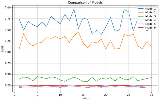
Figure 11.
The MAE value.
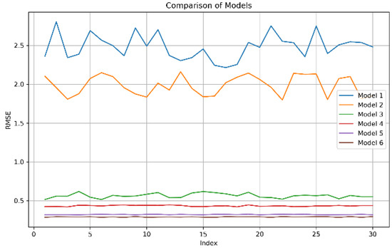
Figure 12.
The RMSE value.
A more intuitive comparison of the various parameters of the models is presented in Table 5, which summarizes the average values for 30 temperature measurement points. Overall, our model performed at a higher level across all indicators, resulting in better predictive performance.
Table 5.
The average values of the metrics for each model.
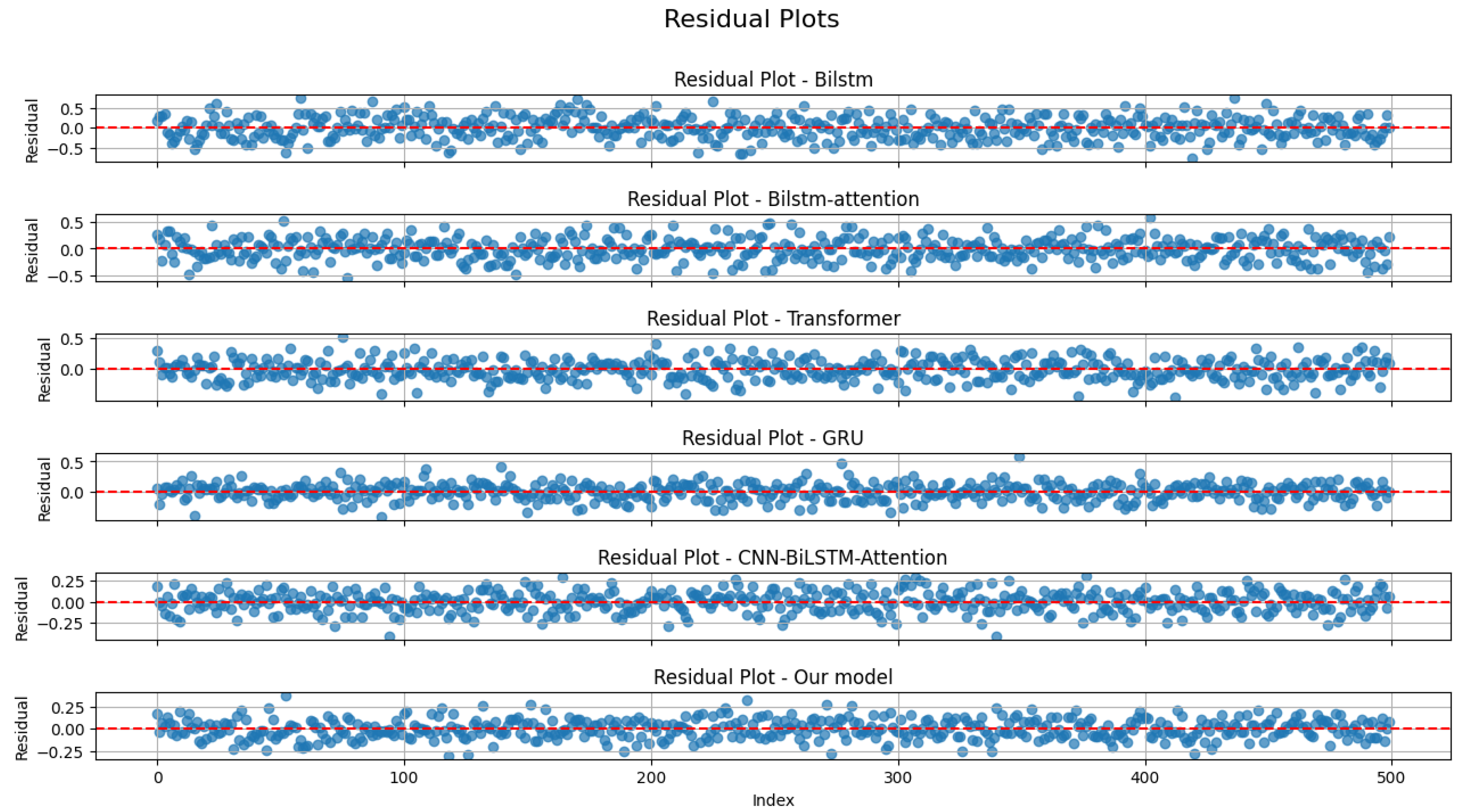
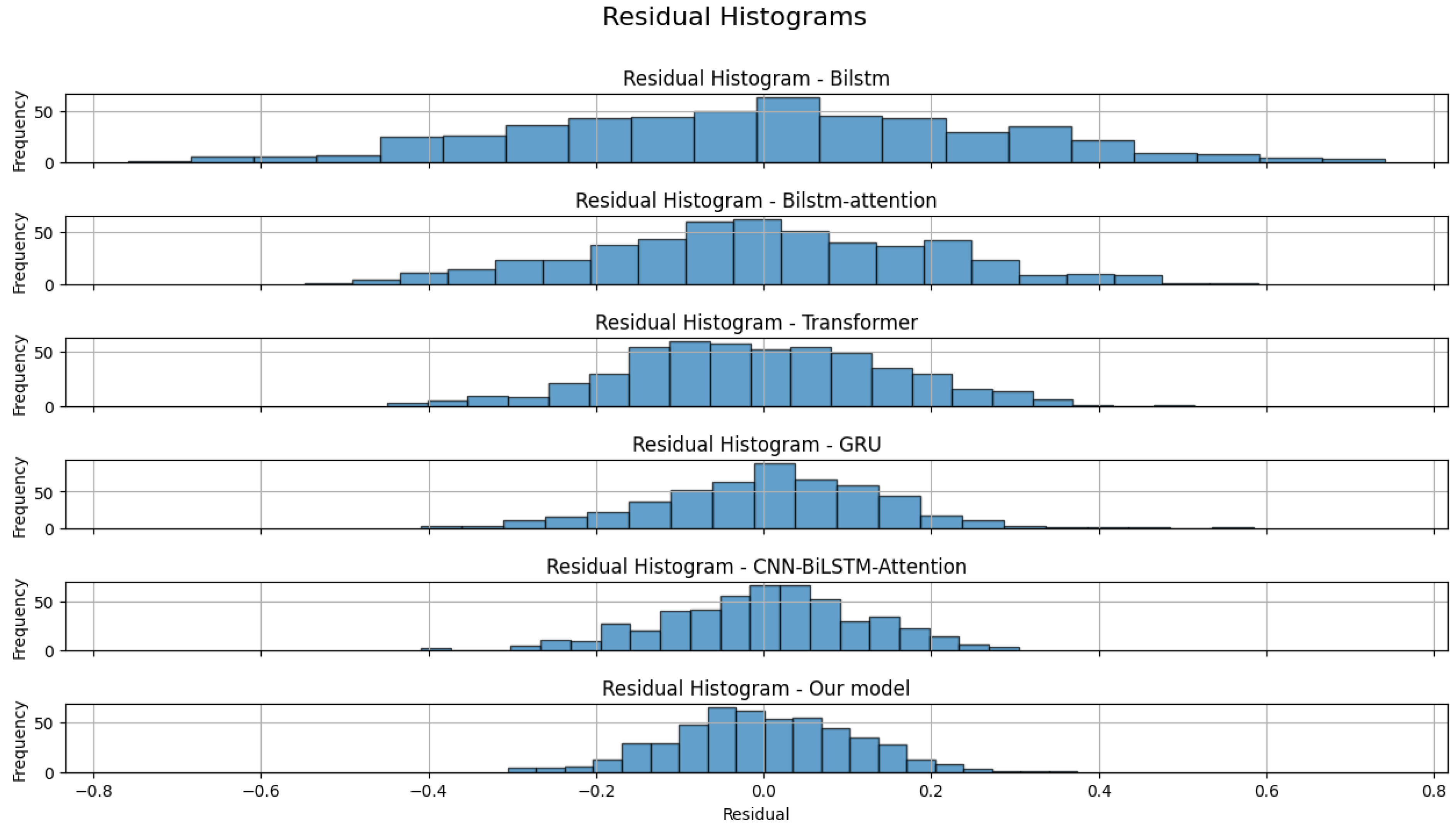
Thirdly, we randomly selected five sets of results for residual analysis. The residual distribution plots for the six models are shown in Figure 13, and the residual histograms are shown in Figure 14. It can be observed that there are no outliers, with all models’ residuals being within ±0.5. Our model and the CNN-BiLSTM-Attention model narrowed the residual range to between ±0.25. The histograms indicate that the residuals of all models are nearly normally distributed. Therefore, we conducted the Anderson–Darling test for normality. The results are presented in Table 6.
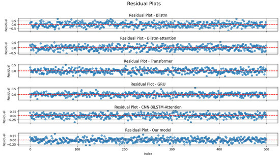
Figure 13.
Residual distribution of six models.
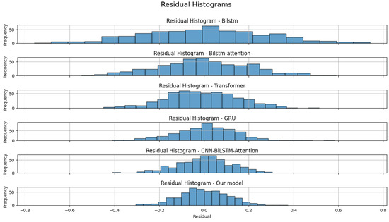
Figure 14.
Histogram of residual distribution for six models.
Table 6.
The Anderson–Darling normality test results for the six models.
Based on the principle of the Anderson–Darling normality test, the models whose residuals are closest to a normal distribution are those with statistics less than the critical values at all significance levels. This indicates that their residuals conform to a normal distribution across all levels. According to the Table 6, the GRU model’s residuals do not conform to a normal distribution at the 15.0%, 10.0%, and 5.0% levels, only conforming at the 2.5% and 1.0% levels. The remaining five models have statistics below the critical values at all significance levels, indicating that their residuals conform to a normal distribution at all significance levels.
Finally, to more clearly demonstrate the effectiveness of each model, we selected data from the temperature sensor points that had the most corrupted data for evaluation, as shown in Figure 15, which displays 500 data points. It can be observed that several basic models performed averagely and exhibited significant fluctuations, indicating high sensitivity to data and inability to adapt to new test data. In contrast, Transformer, GRU, CNN-BiLSTM-Attention, and the proposed model in this paper all achieved relatively good results. Particularly, the proposed model shows a more appropriate prediction of the detailed trend of the data. The results indicate that our proposed model has better generalization performance and practicality.
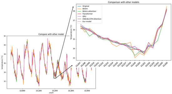
Figure 15.
Testing data on different models.
4. Conclusions
This paper introduced a model for predicting temperature time series, providing a reliable basis for adjusting the elevation of bridge construction sites. The model integrates advanced machine learning techniques, utilizing convolutional neural network (CNN) layers for initial feature extraction and bidirectional long short-term memory (Bi-LSTM) layers to capture temporal dependencies. An attention mechanism enhances the model’s focus during training, allowing it to concentrate on the most relevant parts of the sequence.
The model’s parameters, including the number of LSTM units, dropout rate, and learning rate, were optimized using the CPO algorithm. Experimental results demonstrate that the proposed model outperformed six other models when evaluated on real data from temperature measurement points on the Xuefeng Lake Bridge. Its low sensitivity to data variations enables it to adapt well to different data environments. The model achieved good prediction accuracy and robustness and eliminated the need for manual network parameter tuning, significantly enhancing its practical value in engineering applications. By applying this model to analyze and predict the collected data, the construction or maintenance plans of the bridge can be adjusted in a timely manner. Overall, the model’s ability to accurately predict temperature sequences and its ease of use make it a valuable tool for bridge construction and other engineering applications requiring precise temperature forecasting.
Although this model has shown great potential in practical engineering applications, there is still room for improvement and expansion. Future work can focus on the following areas: first—further optimizing the algorithm to enhance the model’s adaptability to different types of bridges and variable environmental conditions and second—exploring the optimization of more hyperparameters to achieve superior performance.
Author Contributions
Conceptualization, Y.G. and F.G.; Methodology, Y.G., J.W., and F.G.; Software, J.W.; Validation, Y.G.; Formal Analysis, J.W., W.Y., and L.Y.; Investigation, W.Y., L.Y., and F.G.; Resources, W.Y., L.Y., and F.G.; Data Curation, J.W., W.Y., and L.Y.; Writing—Original Draft Preparation, J.W.; Writing—Review and Editing, Y.G.; Visualization, J.W.; Supervision, Y.G.; Project Administration, W.Y. and F.G.; Funding Acquisition, W.Y. and L.Y. All authors have read and agreed to the published version of the manuscript.
Funding
This research was funded by the construction monitoring and technological support unit of the Malukou Zishui Bridge (No: H738012038).
Institutional Review Board Statement
Not applicable.
Informed Consent Statement
Not applicable.
Data Availability Statement
The raw data supporting the conclusions of this article will be made available by the authors on request.
Conflicts of Interest
Authors Wenhao Yu and Lu Yi were employed by the company CCCC Second Harbor Engineering Co., Ltd. The remaining authors declare that the research was conducted in the absence of any commercial or financial relationships that could be construed as a potential conflict of interest.
Correction Statement
This article has been republished with a minor correction to the existing affiliation information. This change does not affect the scientific content of the article.
Appendix A
Appendix A.1
Table A1.
The impact of optimization algorithms on the performance metrics of model prediction results.
Table A1.
The impact of optimization algorithms on the performance metrics of model prediction results.
| Site | CNN-BiLSTM-Attention | CPO-CNN-BiLSTM-Attention | |||||
|---|---|---|---|---|---|---|---|
| 1 | 0.966 | 0.219 | 0.344 | 0.983 | 0.182 | 0.266 | |
| 2 | 0.957 | 0.223 | 0.304 | 0.983 | 0.194 | 0.284 | |
| 3 | 0.946 | 0.197 | 0.307 | 0.990 | 0.186 | 0.300 | |
| 4 | 0.955 | 0.231 | 0.354 | 0.987 | 0.192 | 0.274 | |
| 5 | 0.954 | 0.215 | 0.293 | 0.980 | 0.186 | 0.264 | |
| 6 | 0.958 | 0.190 | 0.345 | 0.979 | 0.187 | 0.284 | |
| 7 | 0.961 | 0.212 | 0.345 | 0.982 | 0.197 | 0.267 | |
| 8 | 0.958 | 0.226 | 0.288 | 0.974 | 0.192 | 0.299 | |
| 9 | 0.950 | 0.217 | 0.298 | 0.969 | 0.183 | 0.292 | |
| 10 | 0.953 | 0.229 | 0.366 | 0.979 | 0.197 | 0.284 | |
| 11 | 0.951 | 0.224 | 0.289 | 0.974 | 0.181 | 0.271 | |
| 12 | 0.965 | 0.202 | 0.338 | 0.979 | 0.186 | 0.288 | |
| 13 | 0.940 | 0.210 | 0.349 | 0.976 | 0.188 | 0.276 | |
| 14 | 0.945 | 0.193 | 0.304 | 0.978 | 0.187 | 0.299 | |
| 15 | 0.950 | 0.231 | 0.320 | 0.974 | 0.194 | 0.268 | |
| 16 | 0.964 | 0.218 | 0.328 | 0.982 | 0.202 | 0.277 | |
| 17 | 0.948 | 0.207 | 0.315 | 0.988 | 0.191 | 0.295 | |
| 18 | 0.960 | 0.225 | 0.341 | 0.974 | 0.185 | 0.302 | |
| 19 | 0.952 | 0.220 | 0.337 | 0.983 | 0.189 | 0.282 | |
| 20 | 0.963 | 0.209 | 0.321 | 0.985 | 0.196 | 0.365 | |
| 21 | 0.949 | 0.224 | 0.357 | 0.980 | 0.203 | 0.298 | |
| 22 | 0.964 | 0.202 | 0.335 | 0.982 | 0.194 | 0.274 | |
| 23 | 0.941 | 0.216 | 0.312 | 0.982 | 0.188 | 0.290 | |
| 24 | 0.955 | 0.228 | 0.348 | 0.973 | 0.191 | 0.307 | |
| 25 | 0.946 | 0.207 | 0.327 | 0.986 | 0.202 | 0.272 | |
| 26 | 0.961 | 0.221 | 0.313 | 0.982 | 0.185 | 0.295 | |
| 27 | 0.937 | 0.198 | 0.340 | 0.984 | 0.198 | 0.271 | |
| 28 | 0.952 | 0.230 | 0.355 | 0.988 | 0.194 | 0.396 | |
| 29 | 0.945 | 0.217 | 0.332 | 0.973 | 0.188 | 0.262 | |
| 30 | 0.958 | 0.203 | 0.319 | 0.986 | 0.191 | 0.283 | |
Appendix A.2
Table A2.
Comparison of between different models.
Table A2.
Comparison of between different models.
| Site | Bi-LSTM | Bi-LSTM-Attention * | Transformer * | GRU * | Our Model |
|---|---|---|---|---|---|
| 1 | 0.87433 | 0.88881 | 0.96347 | 0.96512 | 0.98343 |
| 2 | 0.86245 | 0.89209 | 0.94456 | 0.95924 | 0.98281 |
| 3 | 0.86665 | 0.88945 | 0.95437 | 0.95887 | 0.99022 |
| 4 | 0.86554 | 0.89755 | 0.94864 | 0.96476 | 0.98677 |
| 5 | 0.87221 | 0.88235 | 0.95432 | 0.96543 | 0.98043 |
| 6 | 0.86449 | 0.89112 | 0.96543 | 0.96323 | 0.97864 |
| 7 | 0.87423 | 0.87897 | 0.94552 | 0.94888 | 0.98221 |
| 8 | 0.86999 | 0.88511 | 0.94897 | 0.95732 | 0.97431 |
| 9 | 0.85422 | 0.87553 | 0.94533 | 0.95345 | 0.96943 |
| 10 | 0.86131 | 0.88555 | 0.95342 | 0.94876 | 0.97853 |
| 11 | 0.83511 | 0.82132 | 0.94886 | 0.95443 | 0.97432 |
| 12 | 0.85889 | 0.89181 | 0.96345 | 0.93887 | 0.97866 |
| 13 | 0.86432 | 0.87883 | 0.93995 | 0.96342 | 0.97562 |
| 14 | 0.85764 | 0.86994 | 0.94337 | 0.94543 | 0.97786 |
| 15 | 0.86312 | 0.87443 | 0.95432 | 0.95116 | 0.97434 |
| 16 | 0.85987 | 0.88776 | 0.95227 | 0.96122 | 0.98168 |
| 17 | 0.86229 | 0.89185 | 0.95788 | 0.95758 | 0.98758 |
| 18 | 0.86589 | 0.87787 | 0.94986 | 0.96236 | 0.97384 |
| 19 | 0.87126 | 0.88995 | 0.96125 | 0.95877 | 0.98267 |
| 20 | 0.87368 | 0.89369 | 0.95758 | 0.96168 | 0.98547 |
| 21 | 0.86879 | 0.87757 | 0.95182 | 0.96349 | 0.97968 |
| 22 | 0.87345 | 0.89066 | 0.95348 | 0.96111 | 0.98239 |
| 23 | 0.86776 | 0.88345 | 0.96111 | 0.96486 | 0.98204 |
| 24 | 0.85889 | 0.87126 | 0.94776 | 0.95577 | 0.97267 |
| 25 | 0.87222 | 0.89833 | 0.95988 | 0.96333 | 0.98556 |
| 26 | 0.86555 | 0.88995 | 0.96777 | 0.96111 | 0.98222 |
| 27 | 0.87166 | 0.88223 | 0.95008 | 0.95877 | 0.98389 |
| 28 | 0.86444 | 0.89655 | 0.96292 | 0.96467 | 0.98765 |
| 29 | 0.85889 | 0.87126 | 0.94776 | 0.95577 | 0.97267 |
| 30 | 0.87222 | 0.89833 | 0.95988 | 0.96333 | 0.98556 |
* References [33,34,35] for the experimental model method.
Appendix A.3
Table A3.
Comparison of between different models.
Table A3.
Comparison of between different models.
| Site | Bi-LSTM | Bi-LSTM-Attention | Transformer | GRU | Our Model |
|---|---|---|---|---|---|
| 1 | 2.51426 | 2.07663 | 0.61428 | 0.44754 | 0.26617 |
| 2 | 2.38502 | 1.87753 | 0.51778 | 0.37282 | 0.28363 |
| 3 | 2.50762 | 1.8829 | 0.63639 | 0.39435 | 0.30016 |
| 4 | 2.62975 | 1.95832 | 0.49856 | 0.48252 | 0.27366 |
| 5 | 2.59976 | 2.10168 | 0.49913 | 0.37442 | 0.26357 |
| 6 | 2.43766 | 1.92962 | 0.65953 | 0.43251 | 0.28448 |
| 7 | 2.39612 | 1.94332 | 0.66399 | 0.45368 | 0.26728 |
| 8 | 2.54935 | 2.0775 | 0.54192 | 0.48458 | 0.29876 |
| 9 | 2.61568 | 1.91965 | 0.59939 | 0.48412 | 0.29156 |
| 10 | 2.36867 | 1.94453 | 0.6474 | 0.44203 | 0.28403 |
| 11 | 2.3892 | 2.06006 | 0.49422 | 0.46412 | 0.27097 |
| 12 | 2.52299 | 2.07276 | 0.59683 | 0.39775 | 0.28839 |
| 13 | 2.44284 | 2.12522 | 0.49736 | 0.40745 | 0.27639 |
| 14 | 2.42169 | 1.89827 | 0.49629 | 0.45239 | 0.29923 |
| 15 | 2.51576 | 1.94324 | 0.50344 | 0.41348 | 0.26843 |
| 16 | 2.54289 | 2.01365 | 0.61247 | 0.45976 | 0.27654 |
| 17 | 2.45576 | 1.98167 | 0.58385 | 0.43182 | 0.29459 |
| 18 | 2.63976 | 2.04758 | 0.57386 | 0.49235 | 0.30164 |
| 19 | 2.40826 | 1.92047 | 0.64147 | 0.47162 | 0.28153 |
| 20 | 2.58176 | 2.08333 | 0.53576 | 0.42152 | 0.26495 |
| 21 | 2.47576 | 1.95256 | 0.60285 | 0.44178 | 0.29847 |
| 22 | 2.62876 | 2.07033 | 0.57125 | 0.49133 | 0.27444 |
| 23 | 2.51026 | 1.94153 | 0.63985 | 0.46123 | 0.28954 |
| 24 | 2.38176 | 2.01433 | 0.55976 | 0.43182 | 0.30654 |
| 25 | 2.56976 | 1.98123 | 0.58976 | 0.45123 | 0.27153 |
| 26 | 2.43856 | 2.05233 | 0.61976 | 0.48123 | 0.29544 |
| 27 | 2.54126 | 2.03456 | 0.58975 | 0.46234 | 0.27153 |
| 28 | 2.47889 | 1.95875 | 0.62385 | 0.43856 | 0.29567 |
| 29 | 2.61123 | 2.08223 | 0.54756 | 0.49123 | 0.26237 |
| 30 | 2.38567 | 1.94556 | 0.61248 | 0.47365 | 0.28348 |
Table A4.
Comparison of between different models.
Table A4.
Comparison of between different models.
| Site | Bi-LSTM | Bi-LSTM-Attention | Transformer | GRU | Our Model |
|---|---|---|---|---|---|
| 1 | 1.64677 | 1.2375 | 0.39675 | 0.24478 | 0.18237 |
| 2 | 1.68644 | 1.34472 | 0.35236 | 0.23203 | 0.19445 |
| 3 | 1.52999 | 1.34004 | 0.37323 | 0.22359 | 0.1855 |
| 4 | 1.4836 | 1.12324 | 0.37594 | 0.28901 | 0.19172 |
| 5 | 1.49271 | 1.2169 | 0.3478 | 0.26326 | 0.18556 |
| 6 | 1.43284 | 1.2487 | 0.4357 | 0.25916 | 0.1872 |
| 7 | 1.49353 | 1.31324 | 0.49357 | 0.28681 | 0.19652 |
| 8 | 1.59724 | 1.24848 | 0.37578 | 0.28681 | 0.19235 |
| 9 | 1.41109 | 1.33096 | 0.32472 | 0.24673 | 0.18287 |
| 10 | 1.41370 | 1.12462 | 0.32487 | 0.23145 | 0.19655 |
| 11 | 1.51900 | 1.21041 | 0.36183 | 0.26701 | 0.18123 |
| 12 | 1.51612 | 1.31872 | 0.42554 | 0.23349 | 0.18607 |
| 13 | 1.44502 | 1.14768 | 0.39169 | 0.26147 | 0.18768 |
| 14 | 1.53319 | 1.34334 | 0.28066 | 0.25841 | 0.18694 |
| 15 | 1.60497 | 1.13075 | 0.35165 | 0.25383 | 0.19425 |
| 16 | 1.56388 | 1.25144 | 0.40176 | 0.27765 | 0.20235 |
| 17 | 1.47444 | 1.33225 | 0.36487 | 0.24948 | 0.19116 |
| 18 | 1.59659 | 1.15836 | 0.33549 | 0.28121 | 0.18473 |
| 19 | 1.42233 | 1.26999 | 0.39508 | 0.25272 | 0.18854 |
| 20 | 1.58875 | 1.32055 | 0.31694 | 0.26393 | 0.19642 |
| 21 | 1.57889 | 1.27899 | 0.35208 | 0.28122 | 0.20256 |
| 22 | 1.45233 | 1.32466 | 0.38598 | 0.26237 | 0.19437 |
| 23 | 1.59266 | 1.17224 | 0.31697 | 0.29156 | 0.18758 |
| 24 | 1.43399 | 1.29883 | 0.37224 | 0.25237 | 0.19116 |
| 25 | 1.57667 | 1.31144 | 0.34256 | 0.27256 | 0.20197 |
| 26 | 1.42233 | 1.20599 | 0.39598 | 0.24123 | 0.18474 |
| 27 | 1.58875 | 1.28055 | 0.31693 | 0.28293 | 0.19847 |
| 28 | 1.45123 | 1.32466 | 0.38598 | 0.26237 | 0.19437 |
| 29 | 1.59266 | 1.19883 | 0.31697 | 0.29156 | 0.18758 |
| 30 | 1.43399 | 1.29883 | 0.37224 | 0.25237 | 0.19116 |
References
- Fan, Z.; Huang, Q.; Ren, Y.; Xu, X.; Zhu, Z. Real-time dynamic warning on deflection abnormity of cable-stayed bridges considering operational environment variations. J. Perform. Constr. Facil. 2021, 35, 04020123. [Google Scholar] [CrossRef]
- Catbas, F.N.; Susoy, M.; Frangopol, D.M. Structural health monitoring and reliability estimation: Long span truss bridge application with environmental monitoring data. Eng. Struct. 2008, 30, 2347–2359. [Google Scholar] [CrossRef]
- Lei, X.; Fan, X.; Jiang, H.; Zhu, K.; Zhan, H. Temperature field boundary conditions and lateral temperature gradient effect on a PC box-girder bridge based on real-time solar radiation and spatial temperature monitoring. Sensors 2020, 20, 5261. [Google Scholar] [CrossRef] [PubMed]
- Innocenzi, R.D.; Nicoletti, V.; Arezzo, D.; Carbonari, S.; Gara, F.; Dezi, L. A Good Practice for the Proof Testing of Cable-Stayed Bridges. Appl. Sci. 2022, 12, 3547. [Google Scholar] [CrossRef]
- Li, L.; Shan, Y.; Jing, Q.; Yan, Y.; Xia, Z.; Xia, Y. Global temperature behavior monitoring and analysis of a three-tower cable-stayed bridge. Eng. Struct. 2023, 295, 116855. [Google Scholar] [CrossRef]
- Cao, Y.; Yim, J.; Zhao, Y.; Wang, M.L. Temperature effects on cable-stayed bridge using health monitoring system: A case study. Struct. Health Monit. 2011, 10, 523–537. [Google Scholar] [CrossRef]
- Liu, G.; Yan, D.; Tu, G. Effect of temperature on main beam elevation in construction control of concrete cable-stayed bridge. J. Chang. Univ. Nat. Sci. Ed. 2017, 37, 63–69+77. [Google Scholar] [CrossRef]
- Yue, Z.; Ding, Y.; Zhao, H.; Wang, Z. Case study of deep learning model of temperature-induced deflection of a cable-stayed bridge driven by data knowledge. Symmetry 2021, 13, 2293. [Google Scholar] [CrossRef]
- Box, G.E.P.; Pierce, D.A. Distribution of residual autocorrelations in autoregressive-integrated moving average time series models. J. Am. Stat. Assoc. 1970, 65, 1509–1526. [Google Scholar] [CrossRef]
- Wang, K.; Zhang, Y.; Liu, J.; He, X.; Cai, C.; Huang, S. Prediction of concrete box-girder maximum temperature gradient based on BP neural network. J. Railw. Sci. Eng. 2024, 21, 837–850. [Google Scholar] [CrossRef]
- Shi, X.; Huang, Q.; Chang, J.; Wang, Y.; Lei, J.; Zhao, J. Optimal parameters of the SVM for temperature prediction. Proc. Int. Assoc. Hydrol. Sci. 2015, 368, 162–167. [Google Scholar] [CrossRef]
- Rumelhart, D.E.; Hinton, G.E.; Williams, R.J. Learning representations by back-propagating errors. Nature 1986, 323, 533–536. [Google Scholar] [CrossRef]
- Lipton, Z.C.; Berkowitz, J.; Elkan, C. A critical review of recurrent neural networks for sequence learning. arXiv 2015, arXiv:1506.00019. [Google Scholar]
- Hochreiter, S.; Schmidhuber, J. Long short-term memory. Neural Comput. 1997, 9, 1735–1780. [Google Scholar] [CrossRef] [PubMed]
- Chung, J.; Gulcehre, C.; Cho, K.H.; Bengio, Y. Empirical evaluation of gated recurrent neural networks on sequence modeling. arXiv 2014, arXiv:1412.3555. [Google Scholar]
- Siami-Namini, S.; Tavakoli, N.; Namin, A.S. A comparison of ARIMA and LSTM in forecasting time series. In Proceedings of the 2018 17th IEEE International Conference on Machine Learning and Applications (ICMLA), Orlando, FL, USA, 17–20 December 2018; pp. 1394–1401. Available online: https://ieeexplore.ieee.org/abstract/document/8614252/ (accessed on 21 May 2024).
- Lakshminarayanan, S.K.; McCrae, J.P. A Comparative Study of SVM and LSTM Deep Learning Algorithms for Stock Market Prediction. In Proceedings of the AICS, Wuhan, China, 12–13 July 2019; pp. 446–457. Available online: https://ceur-ws.org/Vol-2563/aics_41.pdf (accessed on 21 May 2024).
- Li, Y.; Zhu, Z.; Kong, D.; Han, H.; Zhao, Y. EA-LSTM: Evolutionary attention-based LSTM for time series prediction. Knowl.-Based Syst. 2019, 181, 104785. [Google Scholar] [CrossRef]
- Siami-Namini, S.; Tavakoli, N.; Namin, A.S. The performance of LSTM and BiLSTM in forecasting time series. In Proceedings of the 2019 IEEE International Conference on Big Data (Big Data), Los Angeles, CA, USA, 9–12 December 2019; pp. 3285–3292. Available online: https://ieeexplore.ieee.org/abstract/document/9005997/ (accessed on 5 June 2024).
- Liu, G.; Guo, J. Bidirectional LSTM with attention mechanism and convolutional layer for text classification. Neurocomputing 2019, 337, 325–338. [Google Scholar] [CrossRef]
- Wang, Z.; Zhang, W.; Zhang, Y.; Liu, Z. Temperature prediction of flat steel box girders of long-span bridges utilizing in situ environmental parameters and machine learning. J. Bridge Eng. 2022, 27, 04022004. [Google Scholar] [CrossRef]
- Zhang, K.; Huo, X.; Shao, K. Temperature time series prediction model based on time series decomposition and bi-lstm network. Mathematics 2023, 11, 2060. [Google Scholar] [CrossRef]
- Bahdanau, D.; Cho, K.; Bengio, Y. Neural machine translation by jointly learning to align and translate. arXiv 2014, arXiv:1409.0473. [Google Scholar]
- Chen, Q.; Xie, Q.; Yuan, Q.; Huang, H.; Li, Y. Research on a Real-Time Monitoring Method for the Wear State of a Tool Based on a Convolutional Bidirectional LSTM Model. Symmetry 2019, 11, 1233. [Google Scholar] [CrossRef]
- Li, J.; Jin, K.; Zhou, D.; Kubota, N.; Ju, Z. Attention mechanism-based CNN for facial expression recognition. Neurocomputing 2020, 411, 340–350. [Google Scholar] [CrossRef]
- Yu, Z.; Yu, J.; Fan, J.; Tao, D. Multi-modal factorized bilinear pooling with co-attention learning for visual question answering. In Proceedings of the IEEE International Conference on Computer Vision, Venice, Italy, 22–29 October 2017; pp. 1821–1830. Available online: https://openaccess.thecvf.com/content_iccv_2017/html/Yu_Multi-Modal_Factorized_Bilinear_ICCV_2017_paper.html (accessed on 5 June 2024).
- Vaswani, A.; Shazeer, N.; Parmar, N.; Uszkoreit, J.; Jones, L.; Gomez, A.N.; Kaiser, Ł.; Polosukhin, I. Attention is all you need. In Proceedings of the Advances in Neural Information Processing Systems, Long Beach, CA, USA, 4–9 December 2017; Volume 30. Available online: https://proceedings.neurips.cc/paper/2017/file/3f5ee243547dee91fbd053c1c4a845aa-Paper.pdf (accessed on 5 June 2024).
- Jallal, M.A.; Chabaa, S.; El Yassini, A. Air temperature forecasting using artificial neural networks with delayed exogenous input. In Proceedings of the 2019 International Conference on Wireless Technologies, Embedded and Intelligent Systems (WITS), Fez, Morocco, 3–4 April 2019; pp. 1–6. Available online: https://ieeexplore.ieee.org/abstract/document/8723699 (accessed on 5 June 2024).
- Zang, J.; Cao, B.; Hong, Y. Research on the Fiber-to-the-Room Network Traffic Prediction Method Based on Crested Porcupine Optimizer Optimization. Appl. Sci. 2024, 14, 4840. [Google Scholar] [CrossRef]
- Abdel-Basset, M.; Mohamed, R.; Abouhawwash, M. Crested Porcupine Optimizer: A new nature-inspired metaheuristic. Knowl.-Based Syst. 2024, 284, 111257. [Google Scholar] [CrossRef]
- Hou, Y.; Deng, X.; Xia, Y. Precipitation Prediction Based on Variational Mode Decomposition Combined with the Crested Porcupine Optimization Algorithm for Long Short-Term Memory Model. AIP Adv. 2024, 14, 065315. [Google Scholar] [CrossRef]
- Li, S.; Jin, X.; Xuan, Y.; Zhou, X.; Chen, W.; Wang, Y.; Yan, X. Enhancing the locality and breaking the memory bottleneck of Transformer on time series forecasting. Adv. Neural Inf. Process. Syst. 2019, 32. Available online: https://proceedings.neurips.cc/paper/2019/hash/6775a0635c302542da2c32aa19d86be0-Abstract.html (accessed on 5 June 2024).
- Du, J.; Cheng, Y.; Zhou, Q.; Zhang, J.; Zhang, X.; Li, G. Power load forecasting using BiLSTM-attention. IOP Conf. Ser. Earth Environ. Sci. 2020, 440, 032115. [Google Scholar] [CrossRef]
- Zheng, W.; Chen, G. An accurate GRU-based power time-series prediction approach with selective state updating and stochastic optimization. IEEE Trans. Cybern. 2021, 52, 13902–13914. [Google Scholar] [CrossRef]
- Zhou, H.; Zhang, S.; Peng, J.; Zhang, S.; Li, J.; Xiong, H.; Zhang, W. Informer: Beyond efficient Transformer for long sequence time-series forecasting. Proc. Aaai Conf. Artif. Intell. 2021, 35, 11106–11115. [Google Scholar] [CrossRef]


Disclaimer/Publisher’s Note: The statements, opinions and data contained in all publications are solely those of the individual author(s) and contributor(s) and not of MDPI and/or the editor(s). MDPI and/or the editor(s) disclaim responsibility for any injury to people or property resulting from any ideas, methods, instructions or products referred to in the content. |
© 2024 by the authors. Licensee MDPI, Basel, Switzerland. This article is an open access article distributed under the terms and conditions of the Creative Commons Attribution (CC BY) license (https://creativecommons.org/licenses/by/4.0/).