
High-Resolution Identification of Sound Sources Based on Sparse Bayesian Learning with Grid Adaptive Split Refinement
Abstract
:1. Introduction
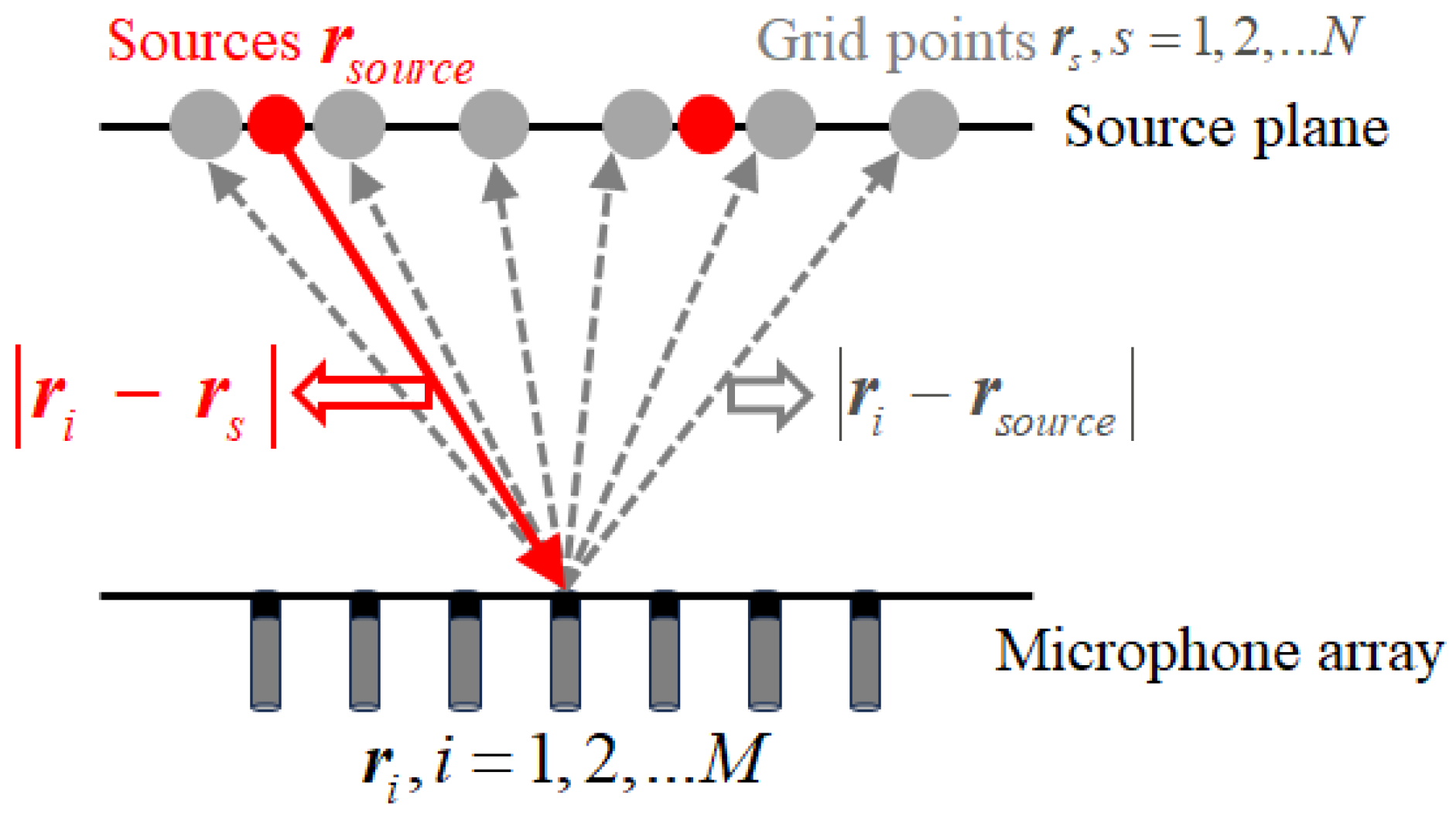
2. Problem Statement
3. Inverse Solving Process
3.1. Sparse Bayesian Learning Solver
3.2. Signal Separation Based on Robust Principal Component Analysis
3.3. Sound Source Identification Method Based on Grid Splitting and Refinement
| Algorithm 1 VG-SBL Algorithm. |
| Input: The snapshot sound pressure: . 1: Discretize the source plane into a grid surface with as the aperture and as the spacing. 2: Establish the transfer matrix between the sound pressure and the source surface. 3: The initial value of the iteration number “” is set to 0. The decay factor and the iteration stopping threshold are set. 4: while . 5: The initial source strength is obtained by sparse Bayesian learning. 6: Split the meshes to update near the local maximum of , with and . 7: Remove duplicate grid points and construct a new transfer model . 8: Form a new sound pressure , and enter it into the MoG-RPCA model. 9: Replace the new sound pressure with the separated low-rank matrix: . 10: . 11: end while Output: The estimation of source strength . |
4. Simulation
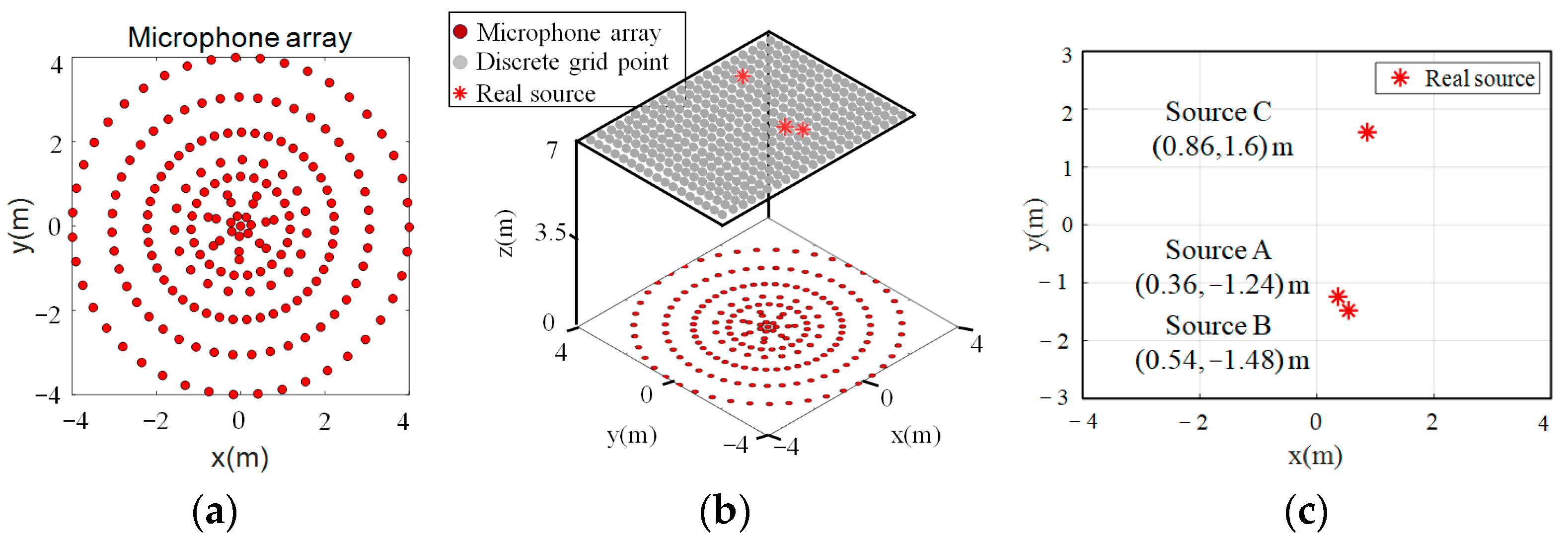
4.1. Simulation Experiment Setup
4.2. Discussion of Results
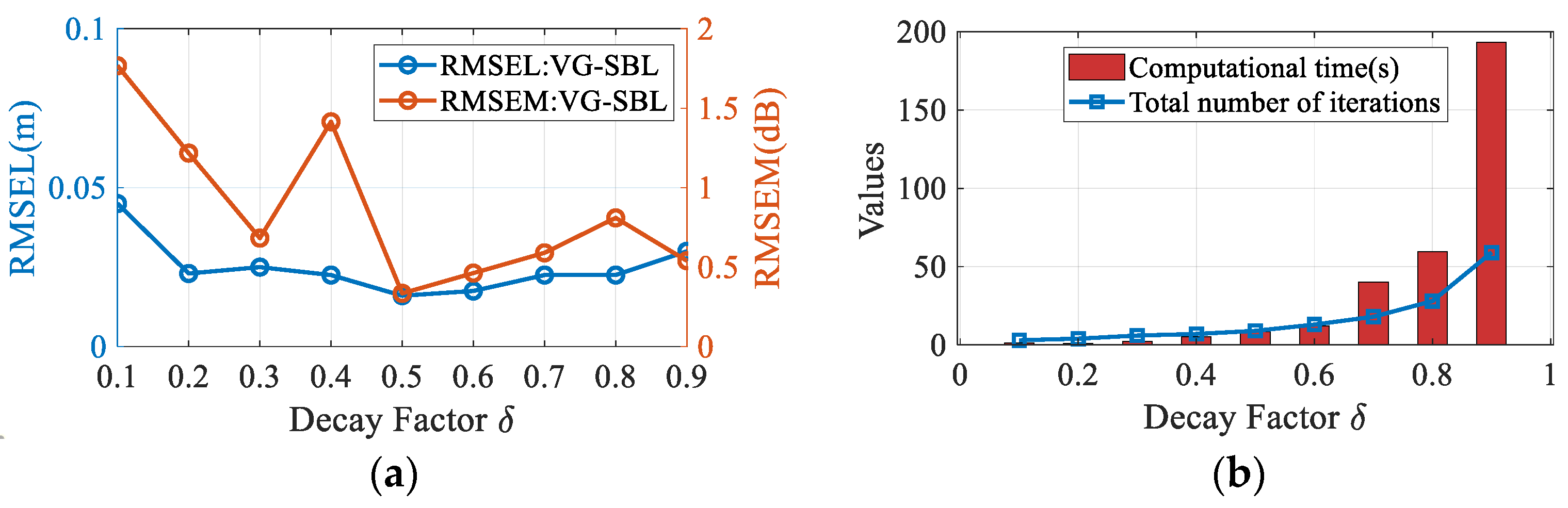
4.2.1. Parameter Discussion
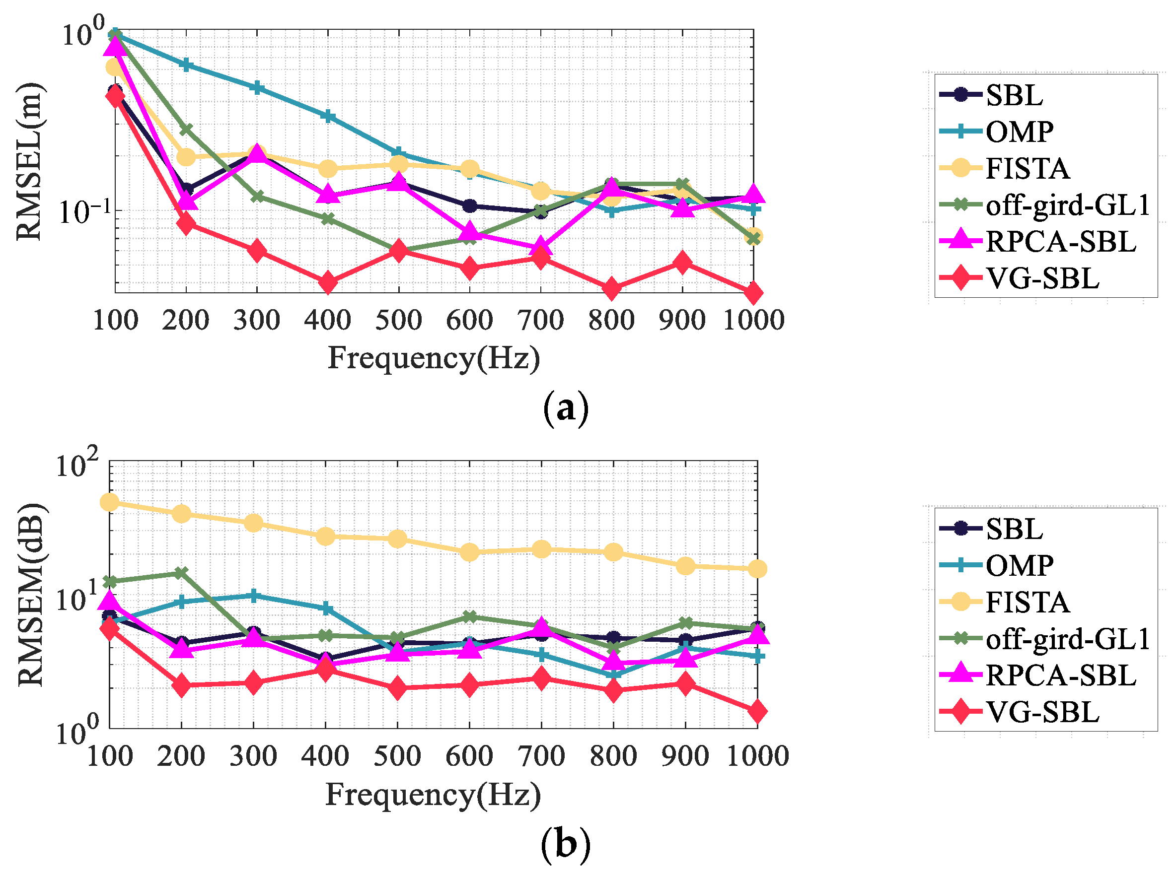
4.2.2. Method Performance Discussion
- (1)
- Influence of source frequency
- (2)
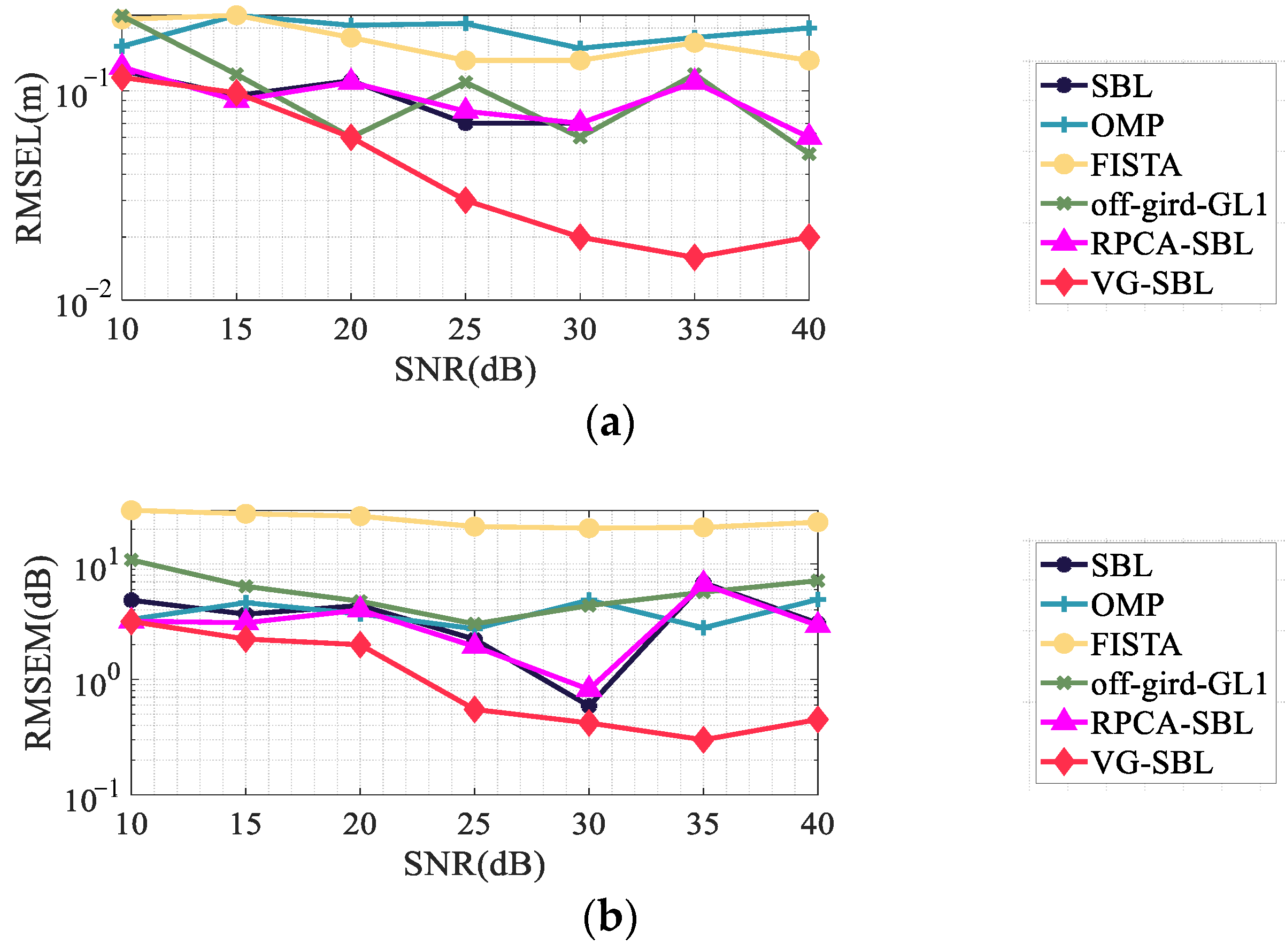
- Influence of SNR
- (3)
- The Impact of Microphone Arrays
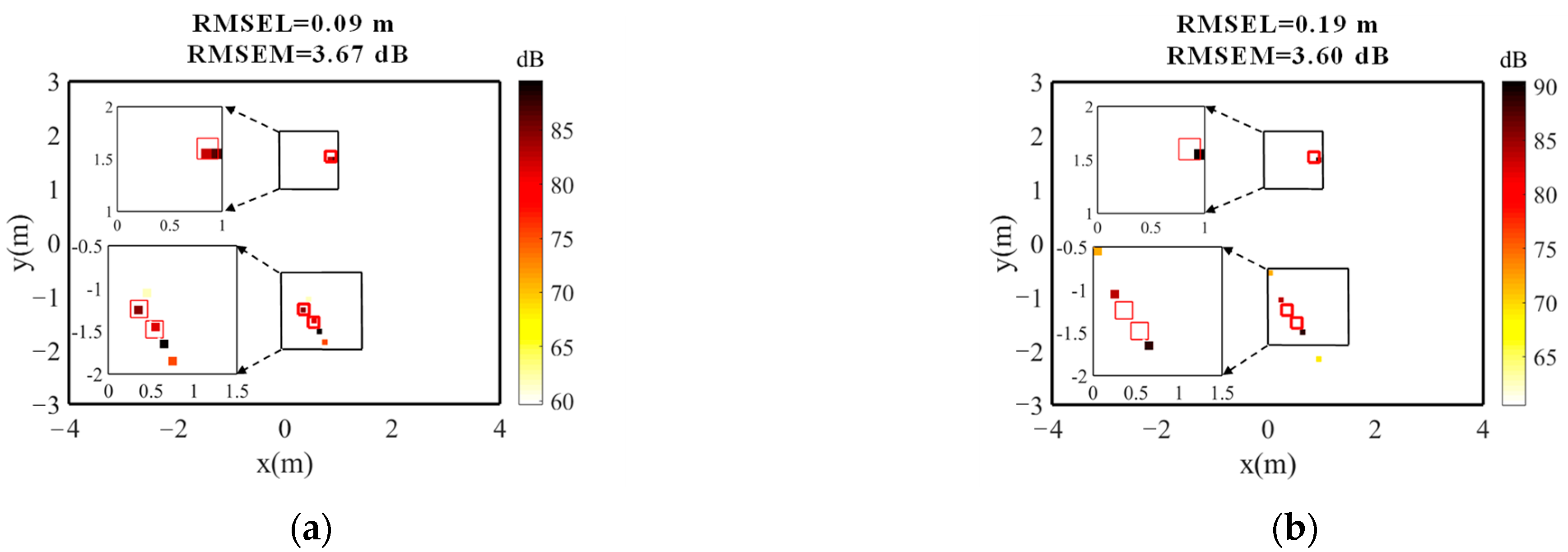
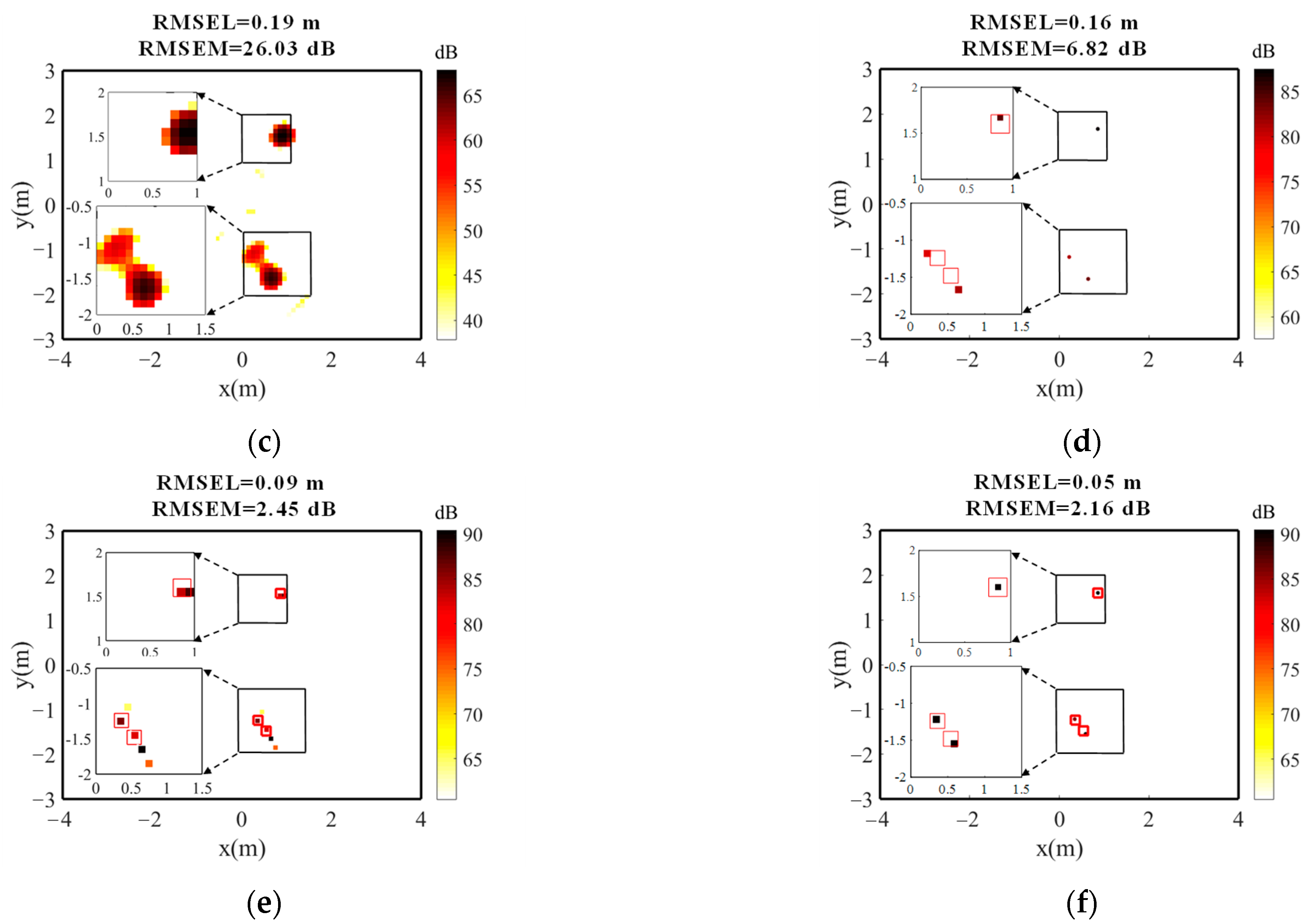
4.2.3. Image Results of Different Methods
4.2.4. Calculation Time Comparison
5. Experimental Validation
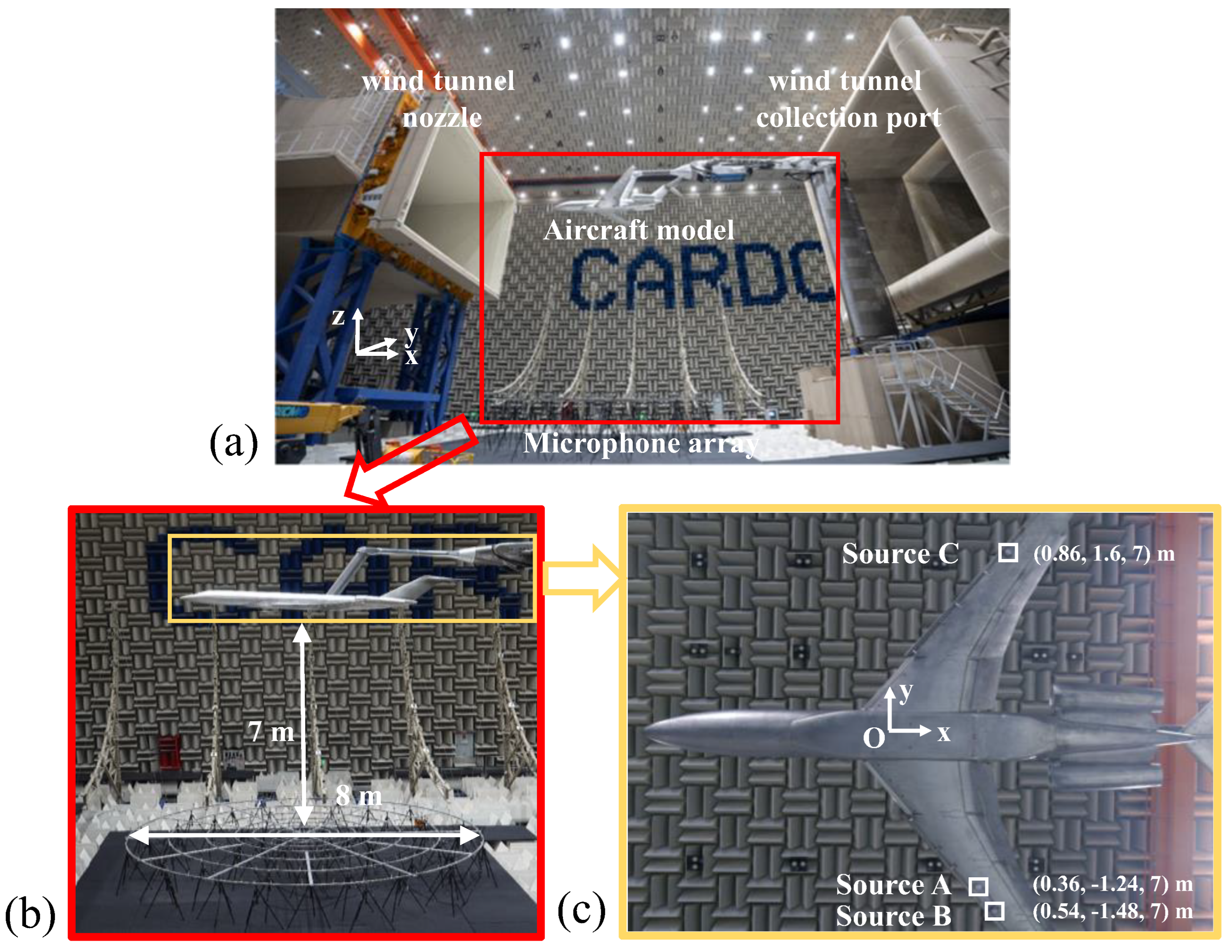
5.1. Experimental Design
5.2. Experimental Results
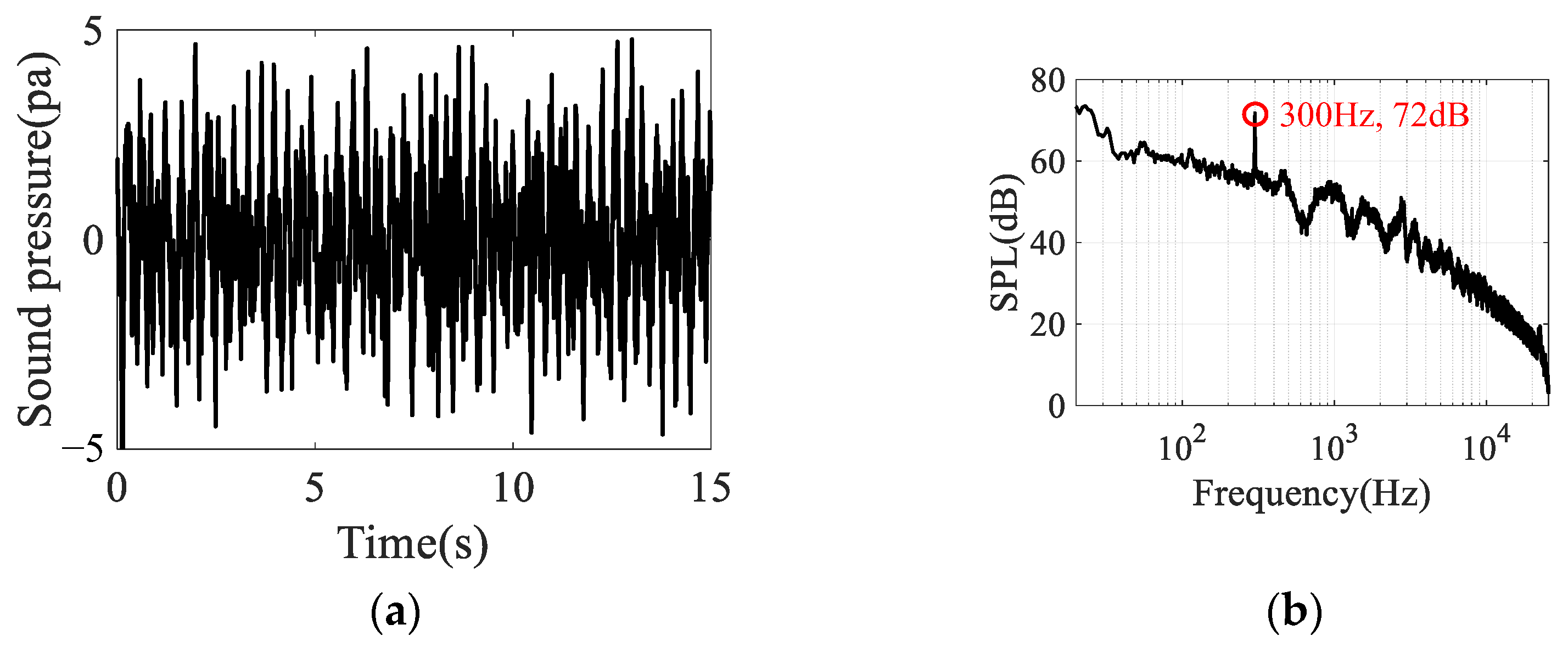
5.2.1. Signal Time–Frequency Analysis
5.2.2. Sound Source Imaging Cloud Maps
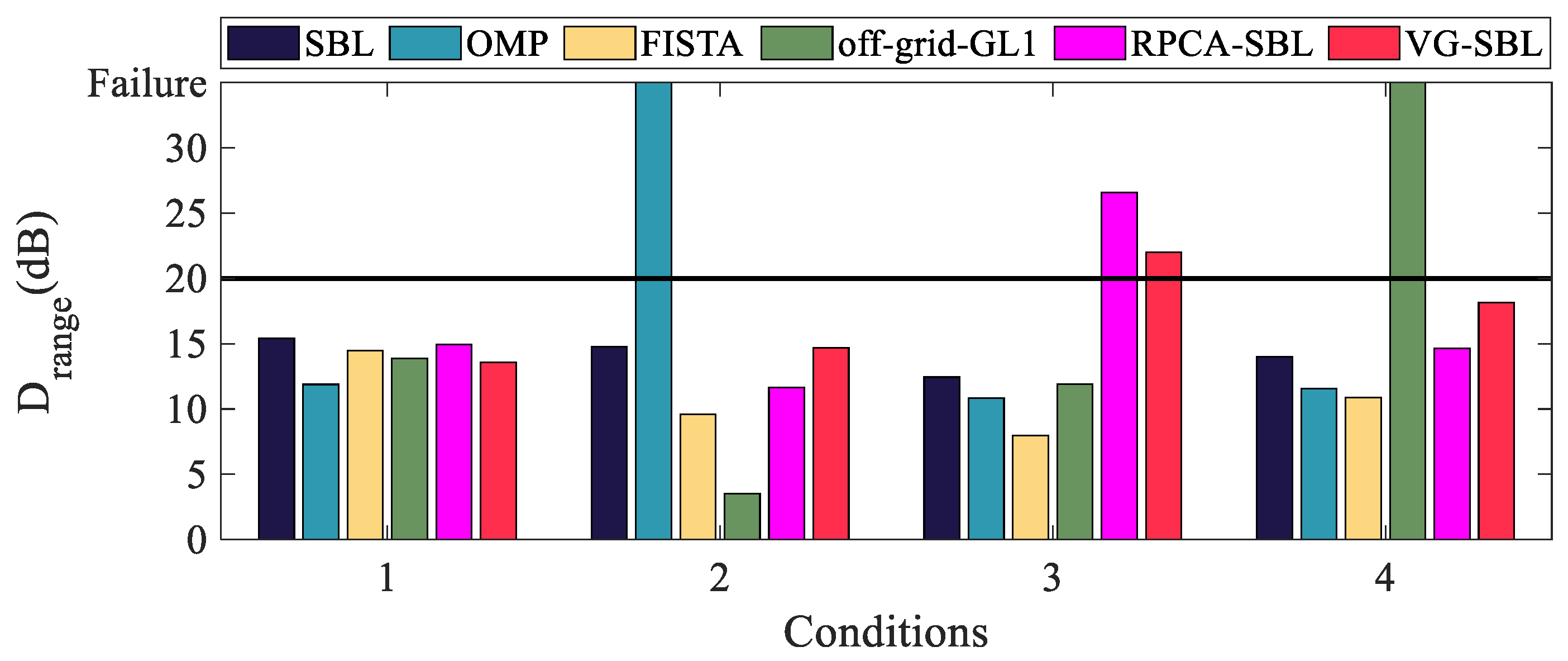
5.2.3. Results
- (1)
- Dynamic range
- (2)
- Location distribution of sound sources
- (3)
- Amplitude error in identification of sound sources
- (4)
- RMSEL and RMSEM
6. Conclusions
Author Contributions
Funding
Institutional Review Board Statement
Informed Consent Statement
Data Availability Statement
Conflicts of Interest
References
- Wang, J.; Ma, W. Deconvolution algorithms of phased microphone arrays for the mapping of acoustic sources in an airframe test. Appl. Acoust. 2020, 164, 107283. [Google Scholar] [CrossRef]
- Merino-Martínez, R.; Luesutthiviboon, S.; Zamponi, R.; Carpio, A.R.; Ragni, D.; Sijtsma, P.; Snellen, M.; Schram, C. Assessment of the accuracy of microphone array methods for aeroacoustic measurements. J. Sound Vib. 2020, 470, 115176. [Google Scholar] [CrossRef]
- Raumer, H.-G.; Spehr, C.; Hohage, T.; Ernst, D. Weighted data spaces for correlation-based array imaging in experimental aeroacoustics. J. Sound Vib. 2021, 494, 115878. [Google Scholar] [CrossRef]
- Battista, G.; Herold, G.; Sarradj, E.; Castellini, P.; Chiariotti, P. IRLS based inverse methods tailored to volumetric acoustic source mapping. Appl. Acoust. 2021, 172, 107599. [Google Scholar] [CrossRef]
- Yu, L.; Zhang, C.; Wang, R.; Yuan, G.; Wang, X. Grid-moving equivalent source method in a probability framework for the transformer discharge fault localization. Measurement 2022, 191, 110800. [Google Scholar] [CrossRef]
- Ma, H.; Duan, M.; Yao, C.; Wang, W.; Feng, J.; Liu, L. Application of acoustic imaging technology in power transformer condition evaluation. In IOP Conference Series: Earth and Environmental Science; IOP Publishing: Bristol, UK, 2020; p. 012043. [Google Scholar]
- Le Courtois, F.; Thomas, J.-H.; Poisson, F.; Pascal, J.-C. Genetic optimisation of a plane array geometry for beamforming. Application to source localisation in a high speed train. J. Sound Vib. 2016, 371, 78–93. [Google Scholar] [CrossRef]
- Zhang, J.; Squicciarini, G.; Thompson, D.J. Implications of the directivity of railway noise sources for their quantification using conventional beamforming. J. Sound Vib. 2019, 459, 114841. [Google Scholar] [CrossRef]
- Ramachandran, R.C.; Raman, G.; Dougherty, R.P. Wind turbine noise measurement using a compact microphone array with advanced deconvolution algorithms. J. Sound Vib. 2014, 333, 3058–3080. [Google Scholar] [CrossRef]
- Chen, Z.M.; Zhu, H.C.; Peng, M. Identification and localization of the sources of cyclostationary sound fields. Appl. Acoust. 2015, 87, 64–71. [Google Scholar] [CrossRef]
- Zhao, L.; Wang, S.; Yang, Y.; Jin, Y.; Zheng, W.; Wang, X. Detection and rapid positioning of abnormal noise of GIS based on acoustic imaging technology. In Proceedings of the 10th Renewable Power Generation Conference (RPG 2021), Online, 14–15 October 2021; pp. 653–657. [Google Scholar]
- Sijtsma, P. Beamforming on Moving Sources; National Aerospace Laboratory NLR: Noordoostpolder, The Netherlands, 2006. [Google Scholar]
- Park, Y.; Seong, W.; Gerstoft, P. Block-sparse two-dimensional off-grid beamforming with arbitrary planar array geometry. J. Acoust. Soc. Am. 2020, 147, 2184–2191. [Google Scholar] [CrossRef]
- Yang, C.; Wang, Y.; Wang, Y.; Hu, D.; Guo, H. An improved functional beamforming algorithm for far-field multi-sound source localization based on Hilbert curve. Appl. Acoust. 2022, 192, 108729. [Google Scholar] [CrossRef]
- Zheng, S.; Tong, F.; Huang, H.; Guo, Q. Exploiting joint sparsity for far-field microphone array sound source localization. Appl. Acoust. 2020, 159, 107100. [Google Scholar] [CrossRef]
- Leclere, Q.; Pereira, A.; Bailly, C.; Antoni, J.; Picard, C. A unified formalism for acoustic imaging techniques: Illustrations in the frame of a didactic numerical benchmark. In Proceedings of the 6th Berlin Beamforming Conference, Berlin, Germany, 29 February–1 March 2016; pp. 1–17. [Google Scholar]
- Nelson, P.A.; Yoon, S.-H. Estimation of acoustic source strength by inverse methods: Part I, conditioning of the inverse problem. J. Sound Vib. 2000, 233, 639–664. [Google Scholar] [CrossRef]
- Xu, Y.; Zhang, X.-Z.; Casalino, D.; Bi, C.-X. Spatial and temporal reconstruction of unsteady rotating forces through an inverse acoustic method. Mech. Syst. Signal Process. 2023, 200, 110596. [Google Scholar] [CrossRef]
- Bell, J.B. Solutions of Ill-Posed Problems; American Mathematical Society: Providence, RI, USA, 1978. [Google Scholar]
- Rubinstein, R.; Zibulevsky, M.; Elad, M. Efficient Implementation of the K-SVD Algorithm Using Batch Orthogonal Matching Pursuit; Citeseer: Forest Grove, OR, USA, 2008. [Google Scholar]
- Efron, B.; Hastie, T.; Johnstone, I.; Tibshirani, R. Least angle regression. Ann. Statist. 2004, 32, 407–499. [Google Scholar] [CrossRef]
- Suzuki, T. L1 generalized inverse beam-forming algorithm resolving coherent/incoherent, distributed and multipole sources. J. Sound Vib. 2011, 330, 5835–5851. [Google Scholar] [CrossRef]
- Presezniak, F.; Zavala, P.A.; Steenackers, G.; Janssens, K.; Arruda, J.R.; Desmet, W.; Guillaume, P. Acoustic source identification using a generalized weighted inverse beamforming technique. Mech. Syst. Signal Process. 2012, 32, 349–358. [Google Scholar] [CrossRef]
- Ping, G.; Chu, Z.; Yang, Y.; Chen, X. Iteratively reweighted spherical equivalent source method for acoustic source identification. IEEE Access 2019, 7, 51513–51521. [Google Scholar] [CrossRef]
- Yu, L.; Antoni, J.; Zhao, H.; Guo, Q.; Wang, R.; Jiang, W. The acoustic inverse problem in the framework of alternating direction method of multipliers. Mech. Syst. Signal Process. 2021, 149, 107220. [Google Scholar] [CrossRef]
- Pereira, A.; Antoni, J.; Leclere, Q. Empirical Bayesian regularization of the inverse acoustic problem. Appl. Acoust. 2015, 97, 11–29. [Google Scholar] [CrossRef]
- Wipf, D.P.; Rao, B.D. Sparse Bayesian learning for basis selection. IEEE Trans. Signal Process. 2004, 52, 2153–2164. [Google Scholar] [CrossRef]
- Bai, Z.; Shi, L.; Jensen, J.R.; Sun, J.; Christensen, M.G. Acoustic DOA estimation using space alternating sparse Bayesian learning. EURASIP J. Audio Speech Music Process. 2021, 2021, 14. [Google Scholar] [CrossRef]
- Gerstoft, P.; Mecklenbräuker, C.F.; Xenaki, A.; Nannuru, S. Multisnapshot sparse Bayesian learning for DOA. IEEE Signal Process. Lett. 2016, 23, 1469–1473. [Google Scholar] [CrossRef]
- Hu, D.-Y.; Liu, X.-Y.; Xiao, Y.; Fang, Y. Fast sparse reconstruction of sound field via Bayesian compressive sensing. J. Vib. Acoust. 2019, 141, 041017. [Google Scholar] [CrossRef]
- Gilquin, L.; Bouley, S.; Antoni, J.; Le Magueresse, T.; Marteau, C. Sensitivity analysis of two inverse methods: Conventional beamforming and Bayesian focusing. J. Sound Vib. 2019, 455, 188–202. [Google Scholar] [CrossRef]
- Ning, F.; Pan, F.; Zhang, C.; Liu, Y.; Li, X.; Wei, J. A highly efficient compressed sensing algorithm for acoustic imaging in low signal-to-noise ratio environments. Mech. Syst. Signal Process. 2018, 112, 113–128. [Google Scholar] [CrossRef]
- Yang, Y.; Chu, Z.; Ping, G. Two-dimensional multiple-snapshot grid-free compressive beamforming. Mech. Syst. Signal Process. 2019, 124, 524–540. [Google Scholar] [CrossRef]
- Xenaki, A.; Gerstoft, P. Grid-free compressive beamforming. J. Acoust. Soc. Am. 2015, 137, 1923–1935. [Google Scholar] [CrossRef]
- Raj, A.G.; McClellan, J.H. Single snapshot super-resolution DOA estimation for arbitrary array geometries. IEEE Signal Process. Lett. 2018, 26, 119–123. [Google Scholar]
- Yang, Y.; Chu, Z.; Xu, Z.; Ping, G. Two-dimensional grid-free compressive beamforming. J. Acoust. Soc. Am. 2017, 142, 618–629. [Google Scholar] [CrossRef]
- Yang, Y.; Chu, Z.; Yang, L.; Zhang, Y. Enhancement of direction-of-arrival estimation performance of spherical ESPRIT via atomic norm minimisation. J. Sound Vib. 2021, 491, 115758. [Google Scholar] [CrossRef]
- Yang, Y.; Chu, Z.; Yin, S. Two-dimensional grid-free compressive beamforming with spherical microphone arrays. Mech. Syst. Signal Process. 2022, 169, 108642. [Google Scholar] [CrossRef]
- Chu, Z.; Liu, Y.; Yang, Y.; Yang, Y. A preliminary study on two-dimensional grid-free compressive beamforming for arbitrary planar array geometries. J. Acoust. Soc. Am. 2021, 149, 3751–3757. [Google Scholar] [CrossRef] [PubMed]
- Wagner, M.; Park, Y.; Gerstoft, P. Gridless DOA Estimation and Root-MUSIC for Non-Uniform Linear Arrays. IEEE Trans. Signal Process. 2021, 69, 2144–2157. [Google Scholar] [CrossRef]
- Yang, Y.; Yang, Y.; Chu, Z.; Shen, L. Multi-frequency synchronous two-dimensional off-grid compressive beamforming. J. Sound Vib. 2022, 517, 116549. [Google Scholar] [CrossRef]
- Yang, Z.; Xie, L.; Zhang, C. Off-grid direction of arrival estimation using sparse Bayesian inference. IEEE Trans. Signal Process. 2012, 61, 38–43. [Google Scholar] [CrossRef]
- Sun, S.; Wang, T.; Chu, F.; Tan, J. Acoustic source identification using an off-grid and sparsity-based method for sound field reconstruction. Mech. Syst. Signal Process. 2022, 170, 108869. [Google Scholar] [CrossRef]
- Wang, R.; Zhuang, T.; Zhang, C.; Jing, Q.; Yu, L.; Xiao, Y. Weighted block ℓ1 norm induced 2D off-grid compressive beamforming for acoustic source localization: Methodology and applications. Appl. Acoust. 2023, 214, 109677. [Google Scholar] [CrossRef]
- Mamandipoor, B.; Ramasamy, D.; Madhow, U. Newtonized orthogonal matching pursuit: Frequency estimation over the continuum. IEEE Trans. Signal Process. 2016, 64, 5066–5081. [Google Scholar] [CrossRef]
- Zan, M.; Xu, Z.; Tang, Z.; Feng, L.; Zhang, Z. Three-dimensional deconvolution beamforming based on the variable-scale compressed computing grid. Measurement 2022, 205, 112211. [Google Scholar] [CrossRef]
- Antoni, J. A Bayesian approach to sound source reconstruction: Optimal basis, regularization, and focusing. J. Acoust. Soc. Am. 2012, 131, 2873–2890. [Google Scholar] [CrossRef] [PubMed]
- Wipf, D.P.; Rao, B.D. An empirical Bayesian strategy for solving the simultaneous sparse approximation problem. IEEE Trans. Signal Process. 2007, 55, 3704–3716. [Google Scholar] [CrossRef]
- Liu, B.; Zhang, Z.; Fan, H.; Fu, Q. Fast marginalized block sparse bayesian learning algorithm. arXiv 2012, arXiv:1211.4909. [Google Scholar]
- Wright, J.; Ganesh, A.; Rao, S.; Peng, Y.; Ma, Y. Robust principal component analysis: Exact recovery of corrupted low-rank matrices via convex optimization. Adv. Neural Inf. Process. Syst. 2009, 22, 2080–2088. [Google Scholar]
- Zhao, Q.; Meng, D.; Xu, Z.; Zuo, W.; Zhang, L. Robust principal component analysis with complex noise. In Proceedings of the International Conference on Machine Learning, Beijing, China, 21–26 June 2014; pp. 55–63. [Google Scholar]
- Pereira, L.T.L.; Merino-Martínez, R.; Ragni, D.; Gómez-Ariza, D.; Snellen, M. Combining asynchronous microphone array measurements for enhanced acoustic imaging and volumetric source mapping. Appl. Acoust. 2021, 182, 108247. [Google Scholar] [CrossRef]
- Luo, X.; Yu, L.; Li, M.; Wang, R.; Yu, H. Complex approximate message passing equivalent source method for sparse acoustic source reconstruction. Mech. Syst. Signal Process. 2024, 217, 111476. [Google Scholar] [CrossRef]
- Wang, R.; Zhang, Y.; Yu, L.; Antoni, J.; Leclère, Q.; Jiang, W. A probability model with Variational Bayesian Inference for the complex interference suppression in the acoustic array measurement. Mech. Syst. Signal Process. 2023, 191, 110181. [Google Scholar] [CrossRef]
- Ning, D.; Sun, C.; Gong, Y.; Zhang, Z.; Hou, J. Extraction of fault component from abnormal sound in diesel engines using acoustic signals. Mech. Syst. Signal Process. 2016, 75, 544–555. [Google Scholar]
- Beck, A.; Teboulle, M. A fast iterative shrinkage-thresholding algorithm for linear inverse problems. SIAM J. Imaging Sci. 2009, 2, 183–202. [Google Scholar] [CrossRef]
- Ahlefeldt, T.; Ernst, D.; Goudarzi, A.; Raumer, H.-G.; Spehr, C. Aeroacoustic testing on a full aircraft model at high Reynolds numbers in the European Transonic Windtunnel. J. Sound Vib. 2023, 566, 117926. [Google Scholar] [CrossRef]
- Salin, M.; Kosteev, D. Nearfield acoustic holography-based methods for far field prediction. Appl. Acoust. 2020, 159, 107099. [Google Scholar] [CrossRef]
- Merino-Martínez, R.; Sijtsma, P.; Snellen, M.; Ahlefeldt, T.; Antoni, J.; Bahr, C.J.; Blacodon, D.; Ernst, D.; Finez, A.; Funke, S. A review of acoustic imaging methods using phased microphone arrays: Part of the “Aircraft Noise Generation and Assessment” Special Issue. CEAS Aeronaut. J. 2019, 10, 197–230. [Google Scholar] [CrossRef]
- Chiariotti, P.; Martarelli, M.; Castellini, P. Acoustic beamforming for noise source localization–Reviews, methodology and applications. Mech. Syst. Signal Process. 2019, 120, 422–448. [Google Scholar] [CrossRef]
- Bahr, C.J.; Humphreys, W.M.; Ernst, D.; Ahlefeldt, T.; Spehr, C.; Pereira, A.; Leclère, Q.; Picard, C.; Porteous, R.; Moreau, D. A comparison of microphone phased array methods applied to the study of airframe noise in wind tunnel testing. In Proceedings of the 23rd AIAA/CEAS Aeroacoustics Conference, Denver, CO, USA, 5–9 June 2017; p. 3718. [Google Scholar]
- Yu, L.; Antoni, J.; Wu, H.; Leclere, Q.; Jiang, W. Fast iteration algorithms for implementing the acoustic beamforming of non-synchronous measurements. Mech. Syst. Signal Process. 2019, 134, 106309. [Google Scholar] [CrossRef]
- Hu, D.; Ding, J.; Zhao, H.; Yu, L. Spatial basis interpretation for implementing the acoustic imaging of non-synchronous measurements. Appl. Acoust. 2021, 182, 108198. [Google Scholar] [CrossRef]
- Morata, D.; Papamoschou, D. Optimized signal processing for microphone arrays containing continuously-scanning sensors. J. Sound Vib. 2022, 537, 117205. [Google Scholar] [CrossRef]
- Sijtsma, P.; Oerlemans, S.; Holthusen, H. Location of rotating sources by phased array measurements. In Proceedings of the 7th AIAA/CEAS Aeroacoustics Conference and Exhibit, Maastricht, The Netherlands, 28–30 May 2001; p. 2167. [Google Scholar]


| Method | Average RMSEL (m) | Average RMSEM (dB) |
|---|---|---|
| SBL | 0.16 | 4.82 |
| OMP | 0.32 | 5.42 |
| FISTA | 0.20 | 27.11 |
| Off-grid-GL1 | 0.20 | 6.94 |
| RPCA-SBL | 0.18 | 4.38 |
| VG-SBL | 0.09 | 2.45 |
| Method | Average RMSEL (m) | Average RMSEM (dB) |
|---|---|---|
| SBL | 0.09 | 3.67 |
| OMP | 0.19 | 3.86 |
| FISTA | 0.17 | 23.99 |
| Off-grid-GL1 | 0.11 | 6.04 |
| RPCA-SBL | 0.09 | 3.24 |
| VG-SBL | 0.05 | 1.31 |
| Method | Average RMSEL (m) | Average RMSEM (dB) |
|---|---|---|
| SBL | 0.54 | 4.99 |
| OMP | 0.58 | 7.64 |
| FISTA | 0.49 | 33.99 |
| Off-grid-GL1 | 0.53 | 5.66 |
| RPCA-SBL | 0.55 | 4.62 |
| VG-SBL | 0.25 | 3.23 |
| Source | Sound Pressure Level (dB) |
|---|---|
| Source A | 88.8 |
| Source B | 92.3 |
| Source C | 90.5 |
| Method | Time (s) |
|---|---|
| SBL | 1.51 |
| OMP | 0.04 |
| FISTA | 16.84 |
| Off-grid-GL1 | 28.88 |
| RPCA-SBL | 1.71 |
| VG-SBL | 7.80 |
| Frequency (Hz) | 300 | 500 |
|---|---|---|
| Sound pressure level of Source A (dB) | 106.7 | 107.0 |
| Sound pressure level of Source B (dB) | 106.7 | 107.0 |
| Sound pressure level of Source C (dB) | 86.7 | 87.0 |
Disclaimer/Publisher’s Note: The statements, opinions and data contained in all publications are solely those of the individual author(s) and contributor(s) and not of MDPI and/or the editor(s). MDPI and/or the editor(s) disclaim responsibility for any injury to people or property resulting from any ideas, methods, instructions or products referred to in the content. |
© 2024 by the authors. Licensee MDPI, Basel, Switzerland. This article is an open access article distributed under the terms and conditions of the Creative Commons Attribution (CC BY) license (https://creativecommons.org/licenses/by/4.0/).
Share and Cite
Pan, W.; Feng, D.; Shi, Y.; Chen, Y.; Li, M. High-Resolution Identification of Sound Sources Based on Sparse Bayesian Learning with Grid Adaptive Split Refinement. Appl. Sci. 2024, 14, 7374. https://doi.org/10.3390/app14167374
Pan W, Feng D, Shi Y, Chen Y, Li M. High-Resolution Identification of Sound Sources Based on Sparse Bayesian Learning with Grid Adaptive Split Refinement. Applied Sciences. 2024; 14(16):7374. https://doi.org/10.3390/app14167374
Chicago/Turabian StylePan, Wei, Daofang Feng, Youtai Shi, Yan Chen, and Min Li. 2024. "High-Resolution Identification of Sound Sources Based on Sparse Bayesian Learning with Grid Adaptive Split Refinement" Applied Sciences 14, no. 16: 7374. https://doi.org/10.3390/app14167374