
Research on the Fault Diagnosis Method of Rotating Machinery Based on Improved Variational Modal Decomposition and Probabilistic Neural Network Algorithm
 ,
,
Abstract
:1. Introduction
2. Vibration Signal Processing Method Based on VMD
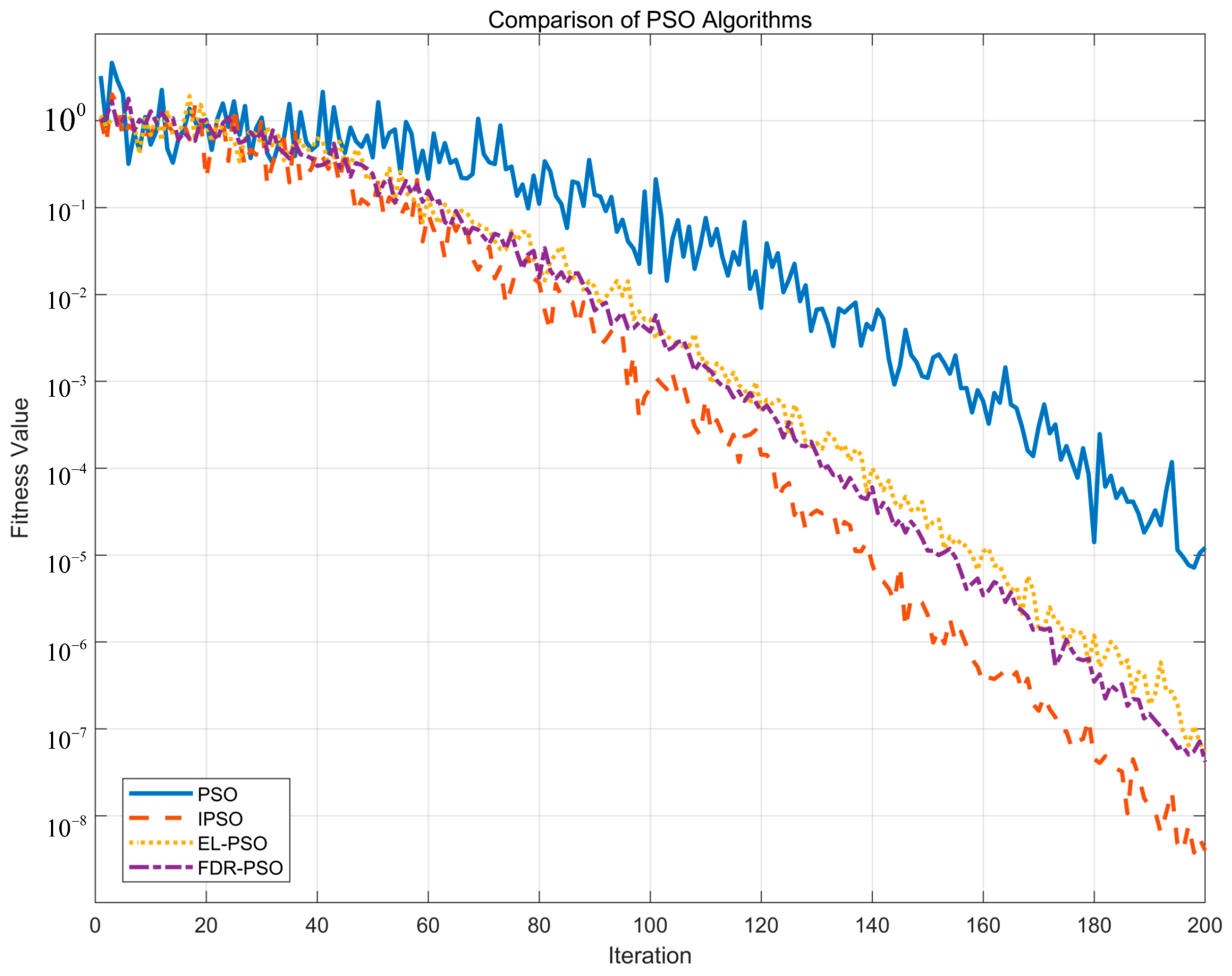
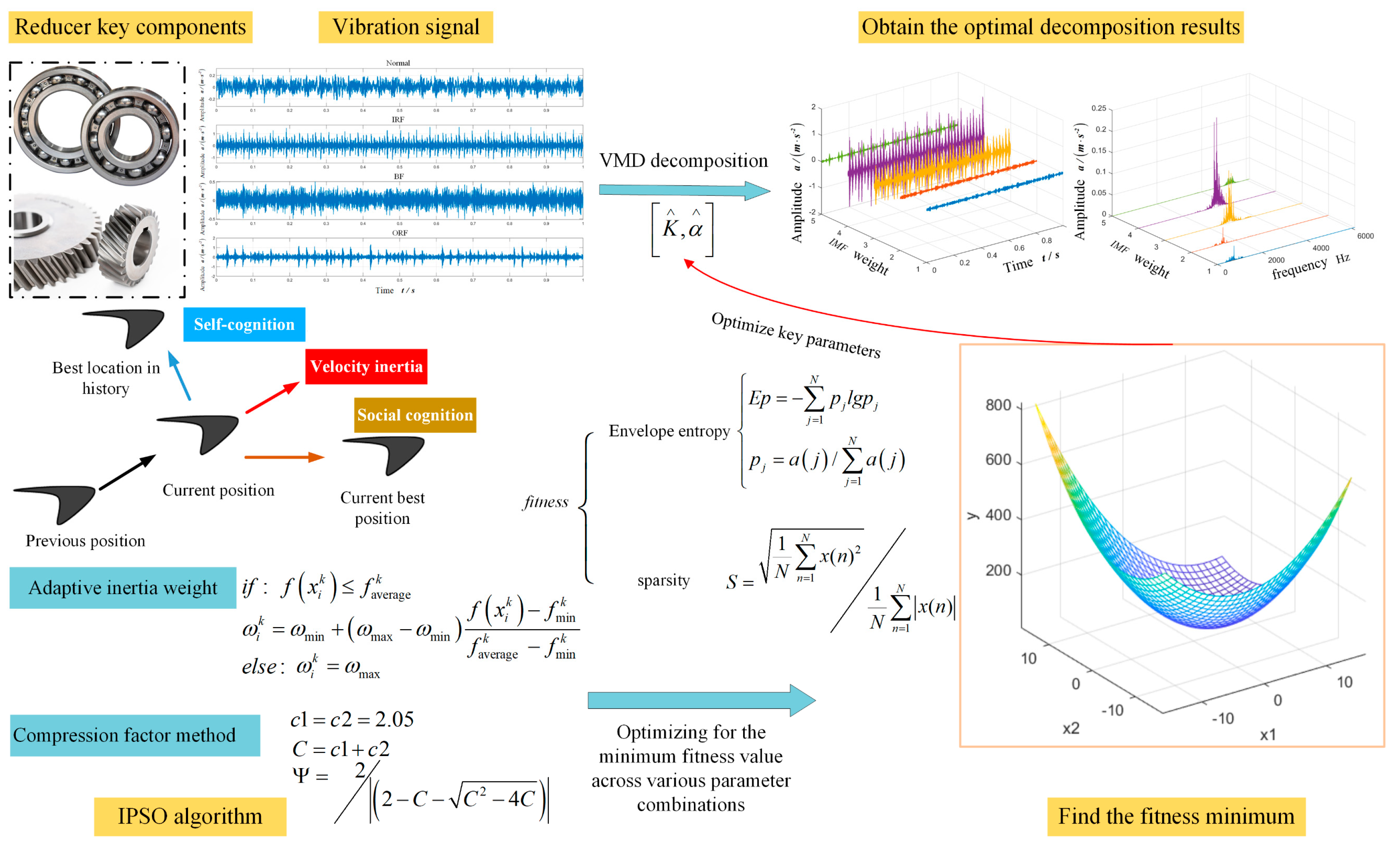
2.1. IPSO-VMD Algorithm Design
- Adaptive inertia weight strategy
- and are the preset minimum and maximum values of inertial weight , taking , ;
- is the average value calculated by the fitness of the whole population at k-th iteration;
- is the minimum fitness of the whole population at iteration.
- 2.
- Compressibility factor method
- 3.
- Elite Learning Strategies
- 4.
- Fitness Distance Ratio Optimization Strategy
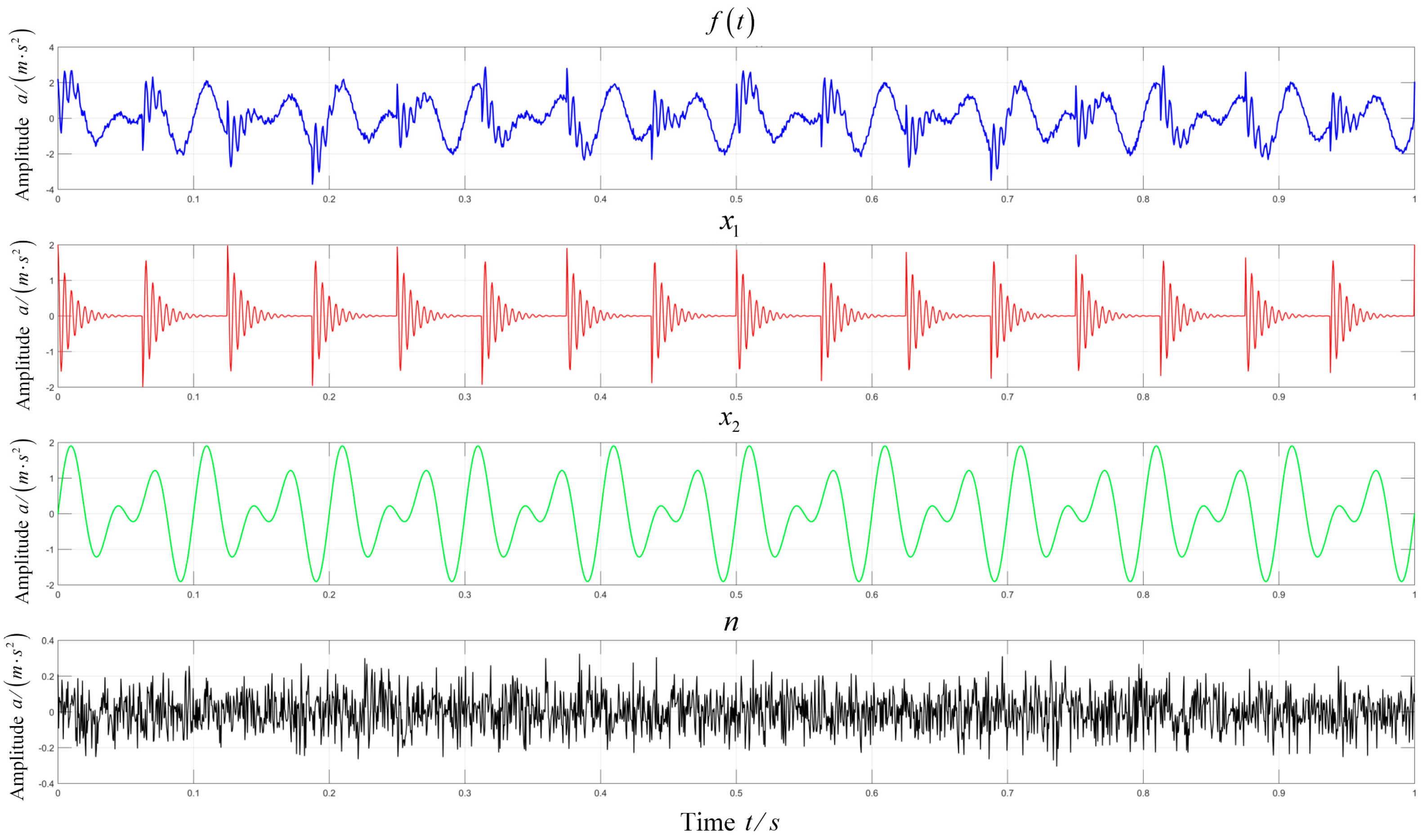
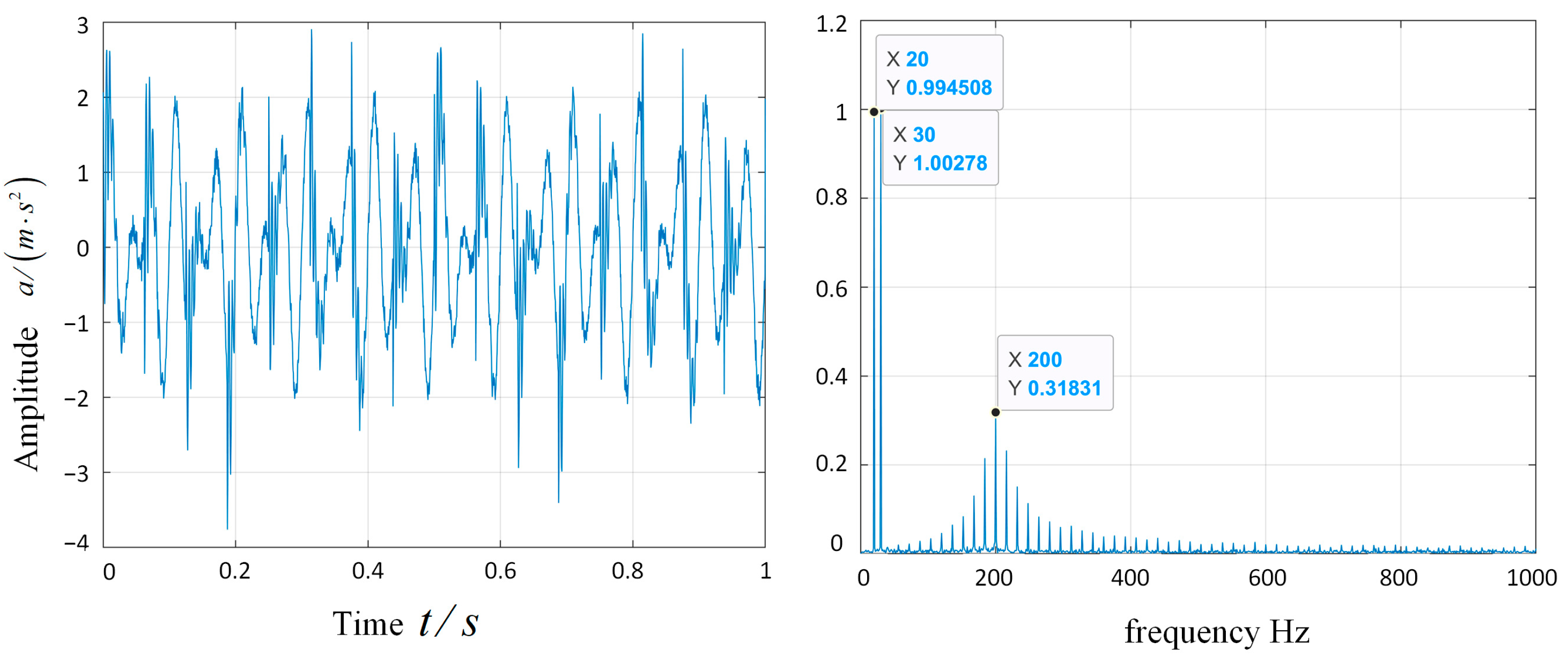
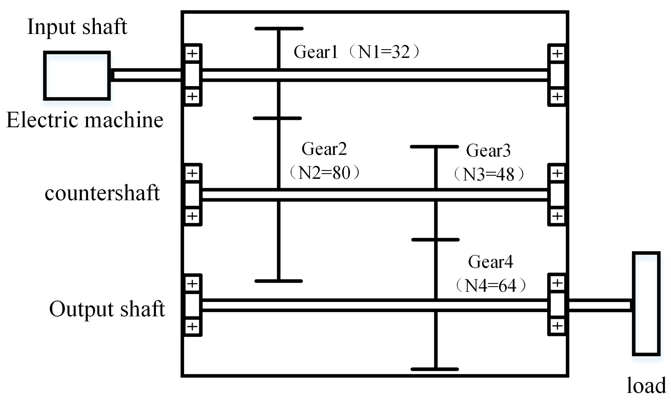
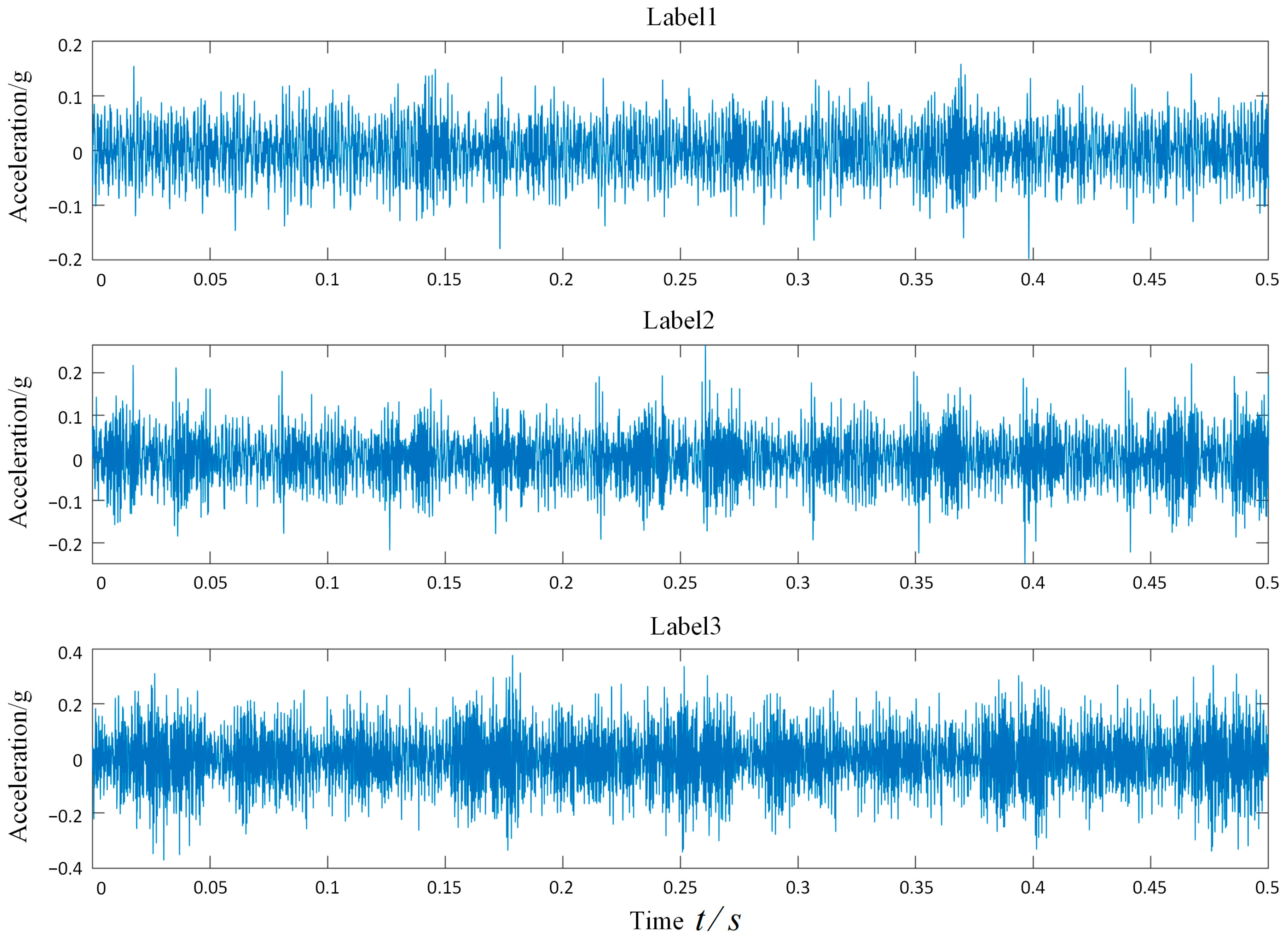
2.2. Fault Simulation Experiment
3. Feature Extraction and Recognition Based on IPSO-VMD
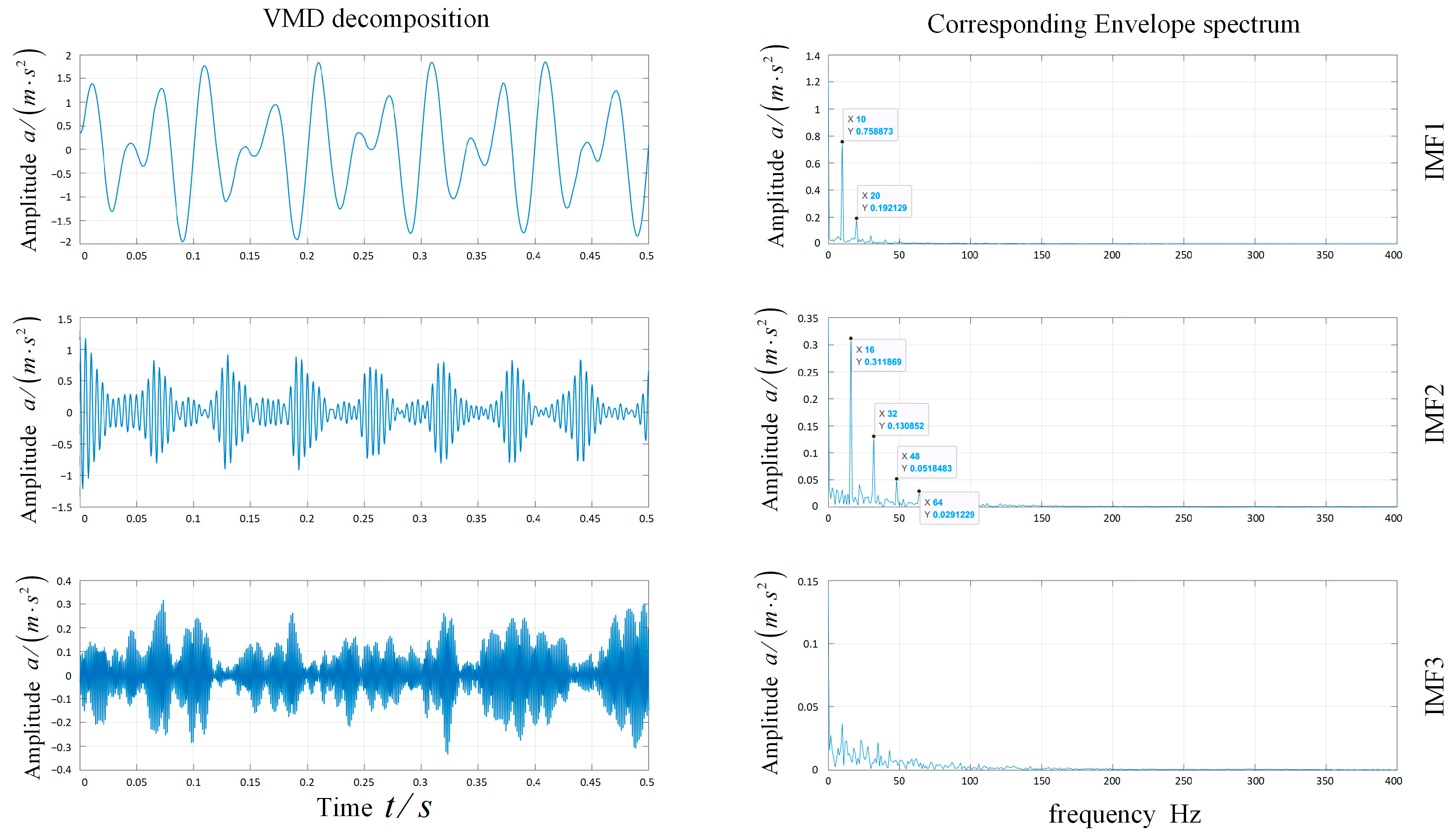
3.1. Feature Extraction Based on VMD
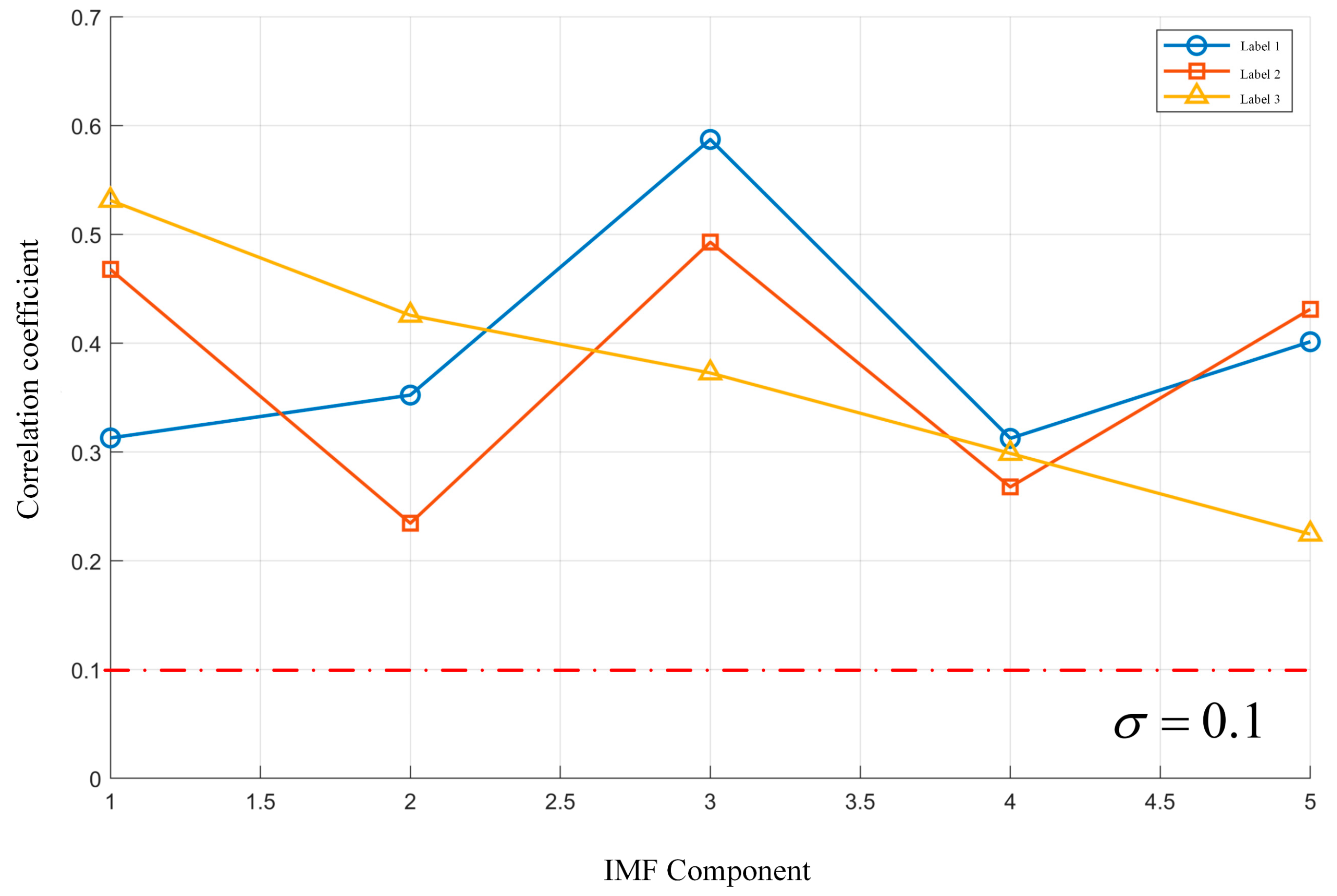
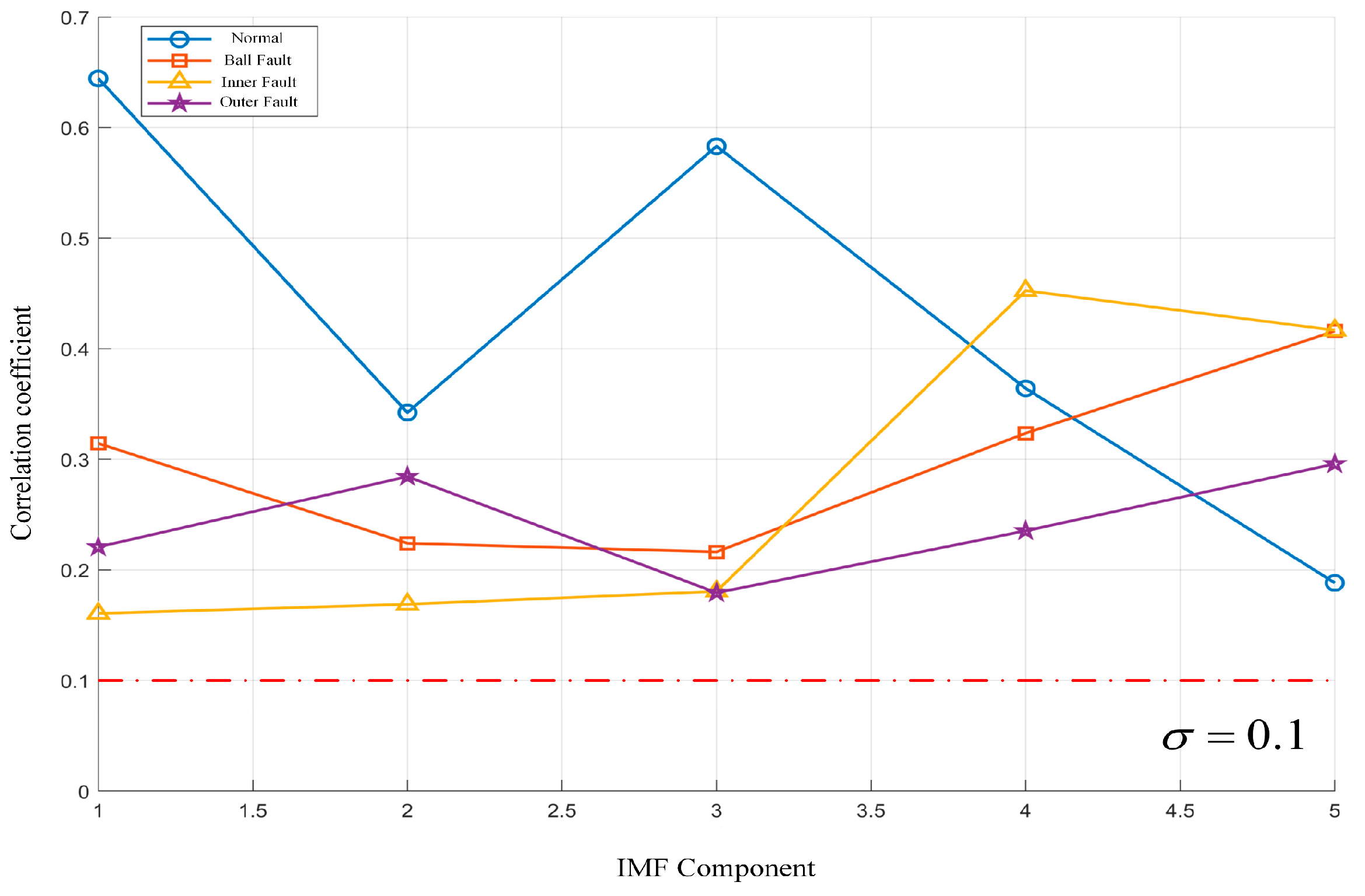
- Correlation Coefficient
- 2.
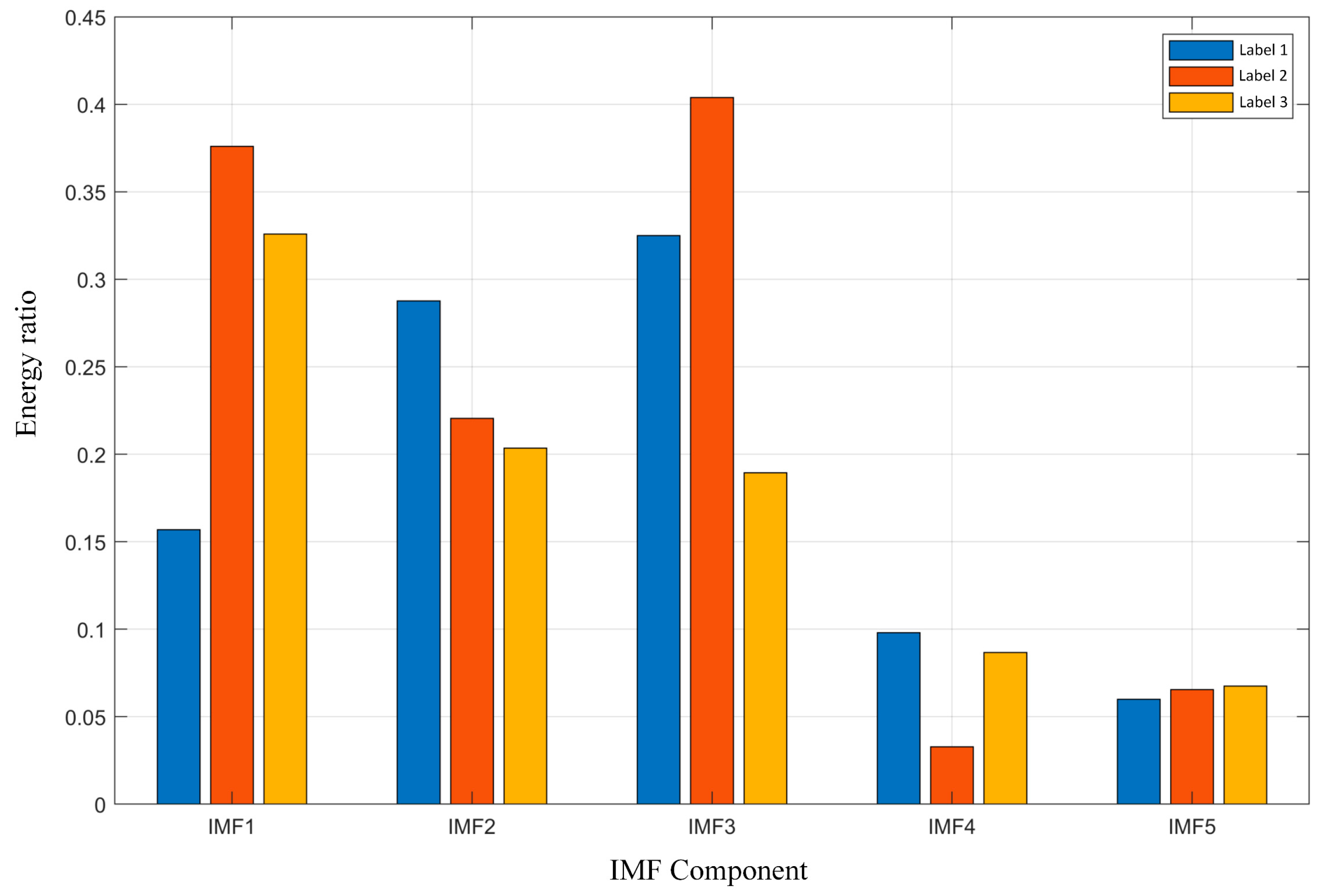
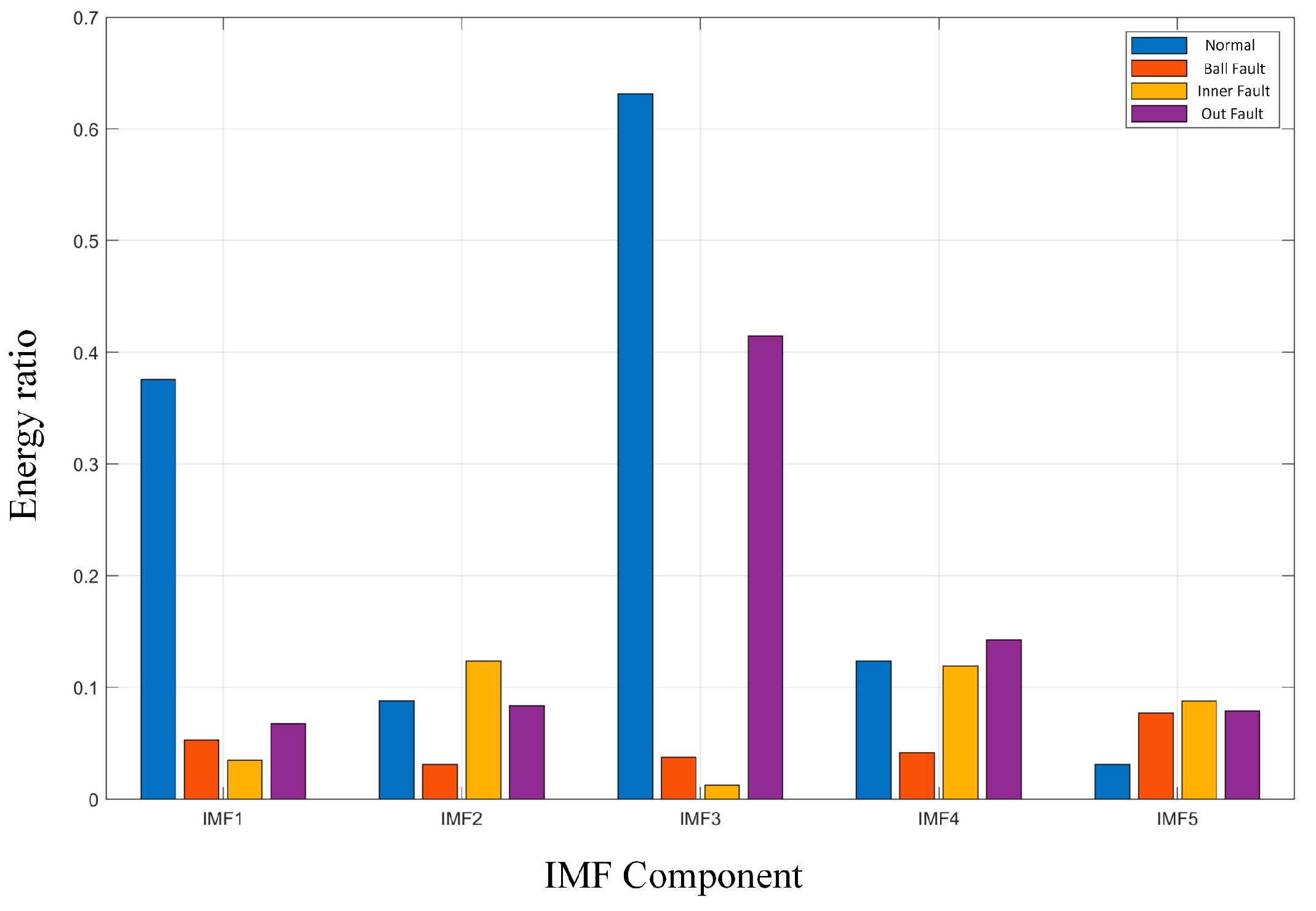
- IMF Energy Ratio
3.2. Multi-Dimension Sensitive Feature Optimization
- Time-Domain Parameters
- 2.
- Frequency-Domain Parameters
- 3.
- Other Parameters
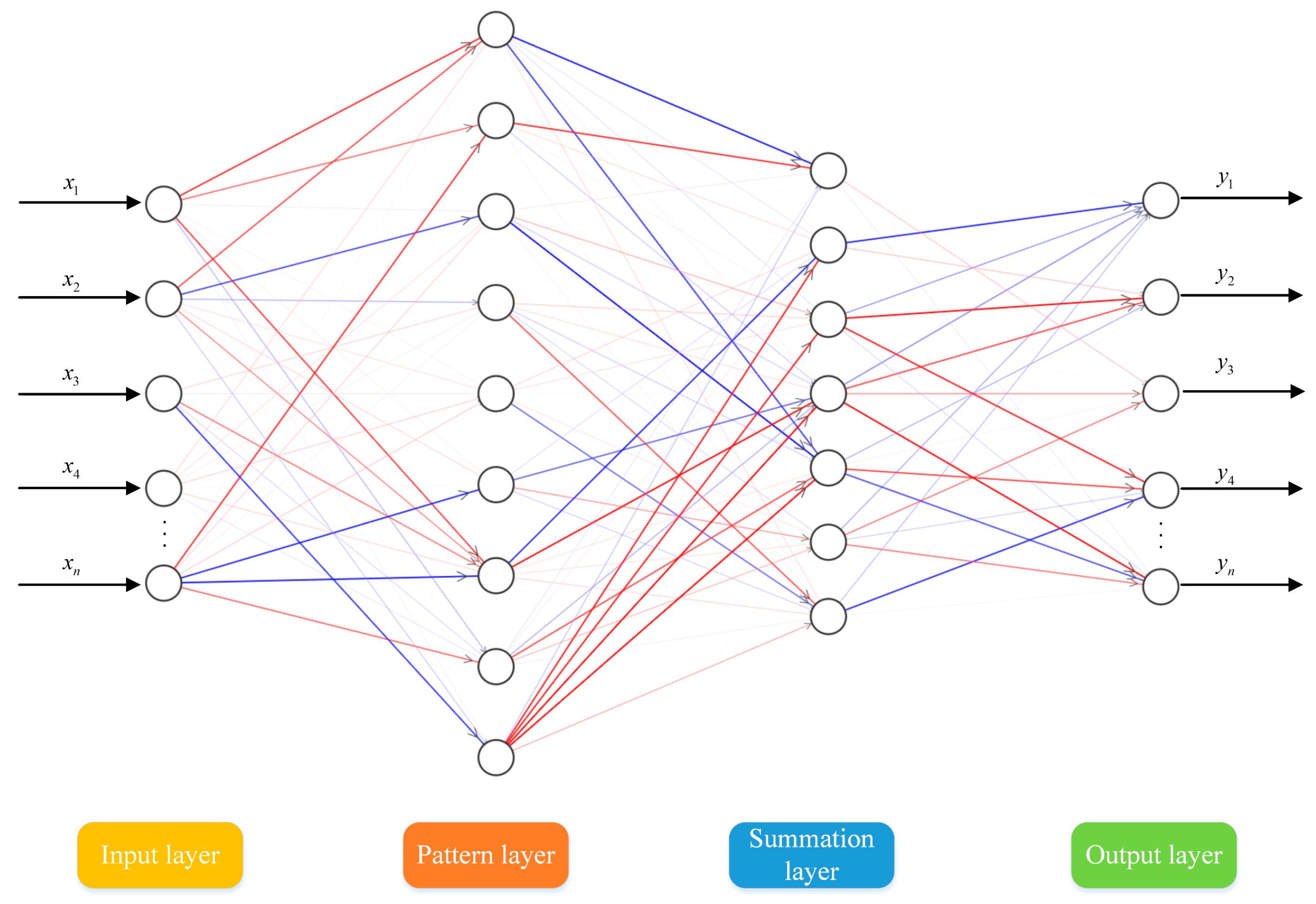
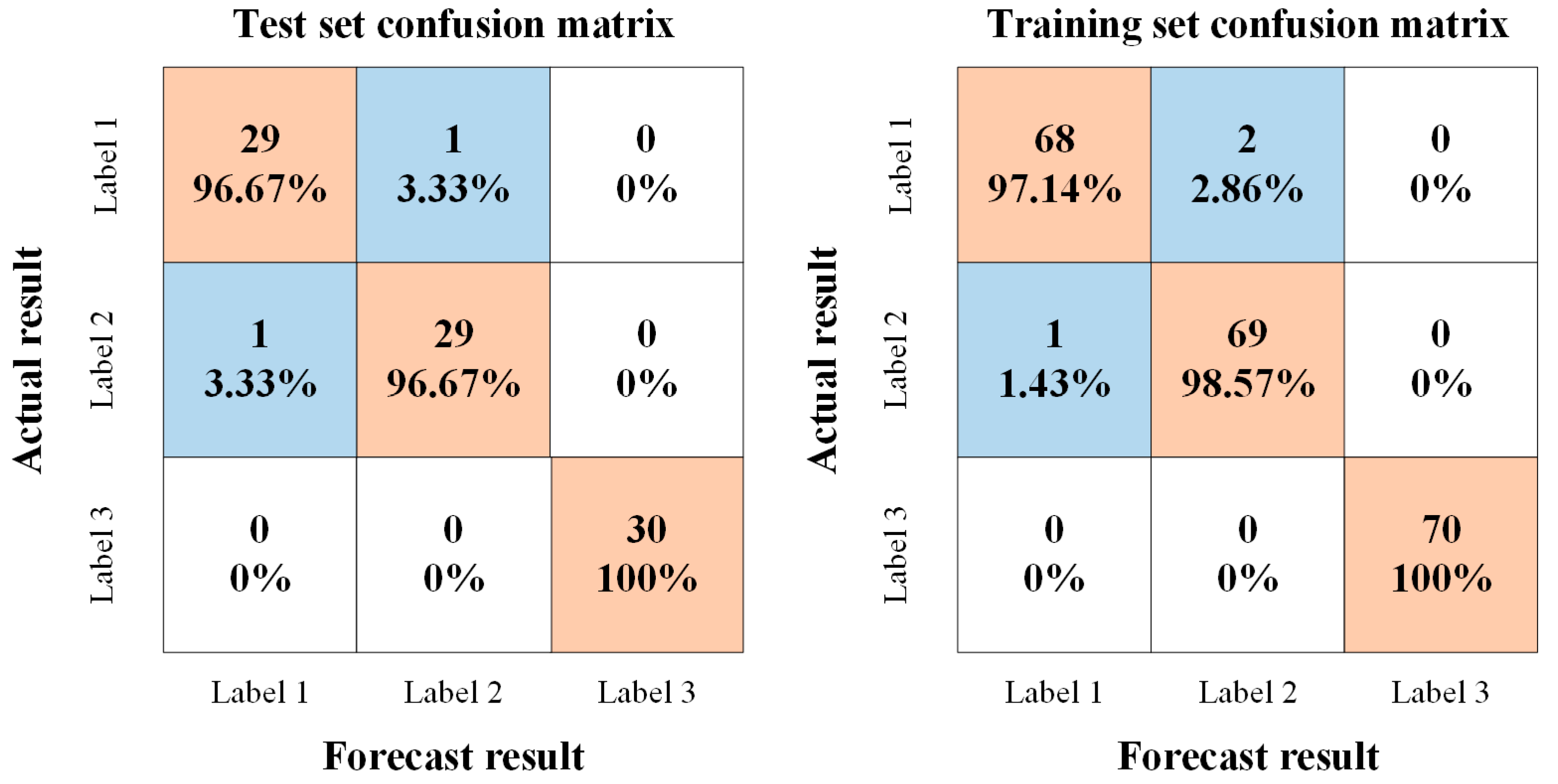
3.3. Probabilistic Neural Networks
4. Experimental Verification
4.1. Case 1
4.2. Case 2
5. Conclusions and Future Work
- In view of the difficulty in selecting the two key parameters and in VMD, the adaptive inertia weight strategy and compression factor method were used to improve the PSO algorithm, and the adaptive optimization of parameters was carried out by combining the fitness function, so as to avoid the instability of manual value taking and cumbersome operation.
- In the extracted multi-dimensional feature vectors, the sensitivity of different fault feature parameters varies, and some parameters may be irrelevant or redundant. Laplace score was used to select sensitive feature parameters from multi-domain feature parameters, and the fault sensitive feature vector was constructed and input into the PNN model to realize fault diagnosis.
- Through the validation of simulated and real signals, the proposed IPSO-VMD-PNN framework shows excellent robustness and adaptability, demonstrating its potential for application in practical engineering.
Author Contributions
Funding
Institutional Review Board Statement
Informed Consent Statement
Data Availability Statement
Conflicts of Interest
References
- Desnica, E.; Ašonja, A.; Radovanović, L.; Palinkaš, I.; Kiss, I. Selection, Dimensioning and Maintenance of Roller Bearings. In 31st International Conference on Organization and Technology of Maintenance (OTO 2022); Lecture Notes in Networks and Systems; Blažević, D., Ademović, N., Barić, T., Cumin, J., Desnica, E., Eds.; Springer: Cham, Switzerland, 2023; Volume 592. [Google Scholar] [CrossRef]
- Xu, X.; Yan, X.; Yang, K.; Zhao, J.; Sheng, C.; Yuan, C. Review of condition monitoring and fault diagnosis for marine power systems. Transp. Saf. Environ. 2021, 3, 85–102. [Google Scholar]
- Chen, Q.; Dai, S.; Bi, X. Fault diagnosis of rolling bearing based on EEMD. Comput. Simul. 2021, 38, 361–364. [Google Scholar]
- Wang, J.; Du, G.; Zhu, Z.; Shen, C.; He, Q. Fault diagnosis of rotating machines based on the EMD manifold. Mech. Syst. Signal Process. 2020, 135, 106443. [Google Scholar]
- Xu, M.; Yao, H. Fault diagnosis method of wheelset based on EEMD-MPE and support vector machine optimized by quantum-behaved particle swarm algorithm. Measurement 2023, 216, 112923. [Google Scholar]
- Zhao, H.; Li, X.; Liu, Z.; Wen, H.; He, J. A double interpolation and mutation interval reconstruction LMD and its application in fault diagnosis of reciprocating compressor. Appl. Sci. 2023, 13, 7543. [Google Scholar] [CrossRef]
- Goyal, D.; Choudhary, A.; Sandhu, J.K.; Srivastava, P.; Saxena, K.K. An intelligent self-adaptive bearing fault diagnosis approach based on improved local mean decomposition. Int. J. Interact. Des. Manuf. 2022, 16, 1–11. [Google Scholar] [CrossRef]
- Dragomiretskiy, K.; Zosso, D. Variational mode decomposition. IEEE Trans. Signal Process. 2014, 62, 531–544. [Google Scholar]
- Li, F.; Li, R.; Tian, L.; Chen, L.; Liu, J. Data-driven time-frequency analysis method based on variational mode decomposition and its application to gear fault diagnosis in variable working conditions. Mech. Syst. Signal Process. 2019, 116, 462–479. [Google Scholar]
- Lin, S.L. Intelligent fault diagnosis and forecast of time-varying bearing based on deep learning VMD-Densenet. Sensors 2021, 21, 7467. [Google Scholar] [CrossRef] [PubMed]
- Li, L.; Meng, W.; Liu, X.; Fei, J. Research on rolling bearing fault diagnosis based on variational modal decomposition parameter optimization and an improved support vector machine. Electronics 2023, 12, 1290. [Google Scholar] [CrossRef]
- Liu, C.; Wu, Y.; Zhen, C. Rolling bearings fault diagnosis based on variational mode decomposition and fuzzy c means clustering. Proc. CSEE 2015, 35, 3358–3365. [Google Scholar]
- Li, K.; Su, L.; Wu, J.; Wang, H.; Chen, P. A rolling bearing fault diagnosis method based on variational mode decomposition and an improved kernel extreme learning machine. Appl. Sci. 2017, 7, 1004. [Google Scholar] [CrossRef]
- Wang, X.; Yang, Z.; Yan, X. Novel particle swarm optimization-based variational mode decomposition method for the fault diagnosis of complex rotating machinery. IEEE/ASME Trans. Mechatron. 2017, 23, 68–79. [Google Scholar]
- Wang, C.; Li, H.; Huang, G.; Ou, J. Early fault diagnosis for planetary gearbox based on adaptive parameter optimized VMD and singular kurtosis difference spectrum. IEEE Access 2019, 7, 31501–31516. [Google Scholar]
- Xiao, D.; Ding, J.; Li, X.; Huang, L. Gear fault diagnosis based on kurtosis criterion VMD and SOM neural network. Appl. Sci. 2019, 9, 5424. [Google Scholar] [CrossRef]
- Zhang, J.; Ji, J.; Xu, T. A bearing fault diagnosis method based on variational mode decomposition parameter optimization. Sci. Technol. Eng. 2021, 21, 3601–3605. [Google Scholar]
- Zhu, S.; Xia, H.; Peng, B.; Zio, E.; Wang, Z.; Jiang, Y. Feature extraction for early fault detection in rotating machinery of nuclear power plants based on adaptive VMD and Teager energy operator. Ann. Nucl. Energy 2021, 15, 108392. [Google Scholar]
- Zhang, Q.; Chen, S.; Fan, Z.P. Bearing Fault Diagnosis based on Improved Particle Swarm Optimized VMD and SVM models. Adv. Mech. Eng. 2021, 13, 16878140211028451. [Google Scholar]
- Song, X.; Wang, H.; Chen, P. Weighted kurtosis-based VMD and improved frequency-weighted energy operator low-speed bearing-fault diagnosis. Meas. Sci. Technol. 2020, 32, 035016. [Google Scholar]
- Chang, Y.; Bao, G.; Cheng, S.; He, T.; Yang, Q. Improved VMD-KFCM algorithm for the fault diagnosis of rolling bearing vibration signals. IET Signal Process. 2021, 15, 238–250. [Google Scholar]
- Jin, Z.; He, D.; Wei, Z. Intelligent fault diagnosis of train axle box bearing based on parameter optimization VMD and improved DBN. Eng. Appl. Artif. Intell. 2022, 110, 104713. [Google Scholar]
- Sharma, V.; Parey, A. Extraction of weak fault transients using variational mode decomposition for fault diagnosis of gearbox under varying speed. Eng. Fail. Anal. 2020, 107, 104204. [Google Scholar]
- Lv, X.; Zhou, D.; Ma, L.; Zhang, Y.; Tang, Y. An Improved Lagrange Particle Swarm Optimization Algorithm and Its Application in Multiple Fault Diagnosis. Shock Vib. 2020, 2020, 1091548. [Google Scholar]
- Zhu, J.; Wang, C.; Hu, Z.; Kong, F.; Liu, X. Adaptive variational mode decomposition based on artificial fish swarm algorithm for fault diagnosis of rolling bearings. Proc. Inst. Mech. Eng. Part C J. Mech. Eng. Sci. 2017, 231, 635–654. [Google Scholar]
- Liu, Y.; Mu, C.; Kou, W.; Liu, J. A simple multi-population evolutionary algorithm using PSO strategy for constrained engineering design optimization. Int. J. Digit. Content Technol. Appl. 2012, 6, 532–541. [Google Scholar]
- Li, K.; Zhou, G.; Zhai, J.; Li, F.; Shao, M. Improved PSO_AdaBoost ensemble algorithm for imbalanced data. Sensors 2019, 19, 1476. [Google Scholar] [CrossRef] [PubMed]
- Mjahed, S.; El Hadaj, S.; Bouzaachane, K.; Raghay, S. Improved PSO based K-means clustering applied to fault signals diagnosis. In Proceedings of the 2018 International Conference on Control, Automation and Diagnosis (ICCAD), Marrakech, Morocco, 19–21 March 2018; pp. 1–6. [Google Scholar]
- Zhou, S.; Li, G.; Wang, Q.; Zheng, C.; Wen, Y. Improved particle swarm optimization algorithm based driving strategy research for permanent magnet spherical motor. Trans. China Electrotech. Soc. 2023, 38, 166–176+189. [Google Scholar]
- Feng, Z.; Zhang, C.; Li, B. Optimization of MFAC parameters based on improved particle swarm optimization algorithm. Control Eng. China 2021, 28, 766–773. [Google Scholar]
- Yang, J.; He, L.; Fu, S. An improved PSO-based charging strategy of electric vehicles in electrical distribution grid. Appl. Energy 2014, 128, 82–92. [Google Scholar]
- Yan, X.; Xu, Y.; She, D.; Zhang, W. A Bearing Fault Diagnosis Method Based on PAVME and MEDE. Entropy 2021, 23, 1402. [Google Scholar] [CrossRef] [PubMed]
- Peeters, C.; Antoni, J.; Helsen, J. Blind filters based on envelope spectrum sparsity indicators for bearing and gear vibration-based condition monitoring. Mech. Syst. Signal Process. 2020, 138, 106556. [Google Scholar]
- Xu, Y.; Wang, Y.; Lingzhi, W.; Qu, J. Bearing fault detection using an alternative analytic energy operator: A fast and non-filtering method. Meas. Sci. Technol. 2021, 32, 105101. [Google Scholar]
- Yan, X.; Liu, Y.; Huang, D.; Jia, M. A new approach to health condition identification of rolling bearing using hierarchical dispersion entropy and improved Laplacian score. Struct. Health Monit. 2021, 20, 1169–1195. [Google Scholar]
- Ma, J.; Li, Z.; Li, C.; Zhan, L.; Zhang, G.-Z. Rolling bearing fault diagnosis based on refined composite multi-scale approximate entropy and optimized probabilistic neural network. Entropy 2021, 23, 259. [Google Scholar] [CrossRef] [PubMed]
- Jing, L.; Zhao, M.; Li, P.; Xu, X. A convolutional neural network based feature learning and fault diagnosis method for the condition monitoring of gearbox. Measurement 2017, 111, 1–10. [Google Scholar]
- He, C.; Wu, T.; Gu, R.; Jin, Z.; Ma, R.; Qu, H. Rolling bearing fault diagnosis based on composite multiscale permutation entropy and reverse cognitive fruit fly optimization algorithm–extreme learning machine. Measurement 2021, 173, 108636. [Google Scholar]
- Case Western Reserve University (CWRU), Cleveland, Ohio, USA [EB/OL]. Available online: https://engineering.case.edu/bearingdatacenter/download-data-file (accessed on 22 January 2022).


| Acquisition System | Processing Board | Sampling Frequency | Sampling Time | Speed |
|---|---|---|---|---|
| dSPACE | DS1006 | 20 kHz | 10 s | 2820 rpm |
| Label | Gears 1 | Gears 2 | Gears 3 | Gears 4 |
|---|---|---|---|---|
| 1 | Normal | Normal | Normal | Normal |
| 2 | Flake | Normal | Normal | Normal |
| 3 | Pit | Normal | Normal | Normal |
| Label 1 | Label 2 | Label 3 |
|---|---|---|
| Gears Status | Feature Extraction Algorithm | Classification Algorithm | Number of Training Sets | Number of Test Sets | Right | Misjudgment | Accuracy Rates |
|---|---|---|---|---|---|---|---|
| Label 1 | IPSO-VMD | PNN | 70 | 30 | 29 | 1 | 96.67% |
| PSO-VMD | PNN | 70 | 30 | 28 | 2 | 93.33% | |
| PSO-VMD | ELM | 70 | 30 | 26 | 4 | 86.67% | |
| PSO-VMD | SVM | 70 | 30 | 27 | 3 | 90.00% | |
| EMD | PNN | 70 | 30 | 24 | 6 | 80.00% | |
| Label 2 | IPSO-VMD | PNN | 70 | 30 | 29 | 1 | 96.67% |
| PSO-VMD | PNN | 70 | 30 | 27 | 3 | 90.00% | |
| PSO-VMD | ELM | 70 | 30 | 24 | 6 | 80.00% | |
| PSO-VMD | SVM | 70 | 30 | 26 | 4 | 86.67% | |
| EMD | PNN | 70 | 30 | 24 | 6 | 80.00% | |
| Label 3 | IPSO-VMD | PNN | 70 | 30 | 30 | 0 | 100% |
| PSO-VMD | PNN | 70 | 30 | 28 | 2 | 93.33% | |
| PSO-VMD | ELM | 70 | 30 | 26 | 4 | 86.67% | |
| PSO-VMD | SVM | 70 | 30 | 28 | 2 | 93.33% | |
| EMD | PNN | 70 | 30 | 25 | 5 | 83.33% |
| Bearing Status | Fault Diameter (mm) | Rotational Speed (rpm) | Data Labels | Number of Samples | Failure Label |
|---|---|---|---|---|---|
| Normal | 0 | 1750 | Normal_2 | 200 | 1 |
| Rolling element Failure | 0.3556 | 1750 | B014_2 | 200 | 2 |
| Inner ring Failure | 0.3556 | 1750 | IR014_2 | 200 | 3 |
| Outer ring Failure | 0.3556 | 1750 | OR014@6_2 | 200 | 4 |
| Normal | Ball Failure | Inner Failure | Outer Failure |
|---|---|---|---|
| Gears Status | Feature Extraction Algorithm | Classification Algorithm | Number of Training Sets | Number of Test Sets | Right | Misjudgment | Accuracy Rate |
|---|---|---|---|---|---|---|---|
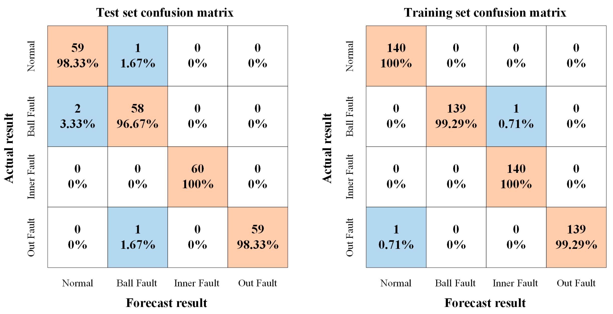
| Normal | IPSO-VMD | PNN | 140 | 60 | 59 | 1 | 98.33% |
| PSO-VMD | PNN | 140 | 60 | 57 | 3 | 95.00% | |
| PSO-VMD | ELM | 140 | 60 | 55 | 5 | 91.67% | |
| PSO-VMD | SVM | 140 | 60 | 58 | 2 | 96.67% | |
| EMD | PNN | 140 | 60 | 54 | 6 | 90.00% | |
| Rolling element failure | IPSO-VMD | PNN | 140 | 60 | 58 | 2 | 96.67% |
| PSO-VMD | PNN | 140 | 60 | 56 | 4 | 93.33% | |
| PSO-VMD | ELM | 140 | 60 | 54 | 6 | 90.00% | |
| PSO-VMD | SVM | 140 | 60 | 57 | 3 | 95.00% | |
| EMD | PNN | 140 | 60 | 53 | 7 | 88.33% | |
| Inner ring Failure | IPSO-VMD | PNN | 140 | 60 | 60 | 0 | 100% |
| PSO-VMD | PNN | 140 | 60 | 59 | 1 | 98.33% | |
| PSO-VMD | ELM | 140 | 60 | 58 | 2 | 96.67% | |
| PSO-VMD | SVM | 140 | 60 | 58 | 2 | 96.67% | |
| EMD | PNN | 140 | 60 | 56 | 4 | 93.33% | |
| Outer ring Failure | IPSO-VMD | PNN | 140 | 60 | 59 | 1 | 98.33% |
| PSO-VMD | PNN | 140 | 60 | 58 | 2 | 96.67% | |
| PSO-VMD | ELM | 140 | 60 | 57 | 3 | 95.00% | |
| PSO-VMD | SVM | 140 | 60 | 58 | 2 | 96.67% | |
| EMD | PNN | 140 | 60 | 55 | 5 | 91.67% |
Disclaimer/Publisher’s Note: The statements, opinions and data contained in all publications are solely those of the individual author(s) and contributor(s) and not of MDPI and/or the editor(s). MDPI and/or the editor(s) disclaim responsibility for any injury to people or property resulting from any ideas, methods, instructions or products referred to in the content. |
© 2024 by the authors. Licensee MDPI, Basel, Switzerland. This article is an open access article distributed under the terms and conditions of the Creative Commons Attribution (CC BY) license (https://creativecommons.org/licenses/by/4.0/).
Share and Cite
Li, Z.; Zou, C.; Chen, Z.; Lu, H.; Xie, S.; Zhang, W.; He, J. Research on the Fault Diagnosis Method of Rotating Machinery Based on Improved Variational Modal Decomposition and Probabilistic Neural Network Algorithm. Appl. Sci. 2024, 14, 7380. https://doi.org/10.3390/app14167380
Li Z, Zou C, Chen Z, Lu H, Xie S, Zhang W, He J. Research on the Fault Diagnosis Method of Rotating Machinery Based on Improved Variational Modal Decomposition and Probabilistic Neural Network Algorithm. Applied Sciences. 2024; 14(16):7380. https://doi.org/10.3390/app14167380
Chicago/Turabian StyleLi, Zhangjie, Chao Zou, Zhimin Chen, Hong Lu, Shiwen Xie, Wei Zhang, and Jiaqi He. 2024. "Research on the Fault Diagnosis Method of Rotating Machinery Based on Improved Variational Modal Decomposition and Probabilistic Neural Network Algorithm" Applied Sciences 14, no. 16: 7380. https://doi.org/10.3390/app14167380