Abstract
Noise in large urban areas, which is mainly generated by road traffic and by the human activities carried out nearby and inside the area under study, is a relevant problem. The continuous exposure to high noise levels, in fact, can lead to several problems, largely documented in the scientific literature. The analysis and forecasting of the noise level in a given area are, then, fundamental for control and prevention, especially when field measurements present peculiar trends and slopes, which can be modeled with a Time Series Analysis approach. In this paper, a hybrid model is presented for the analysis and the forecasting of noise time series in urban areas: this technique is based on the application of a deterministic decomposition model followed in cascade by a predictor of the forecasting errors based on an artificial neural network. Two variants of the hybrid model have been implemented and presented. The time series used to calibrate and validate the model is composed of sound pressure level measurements detected on a busy road near the commercial port of an Italian city. The proposed hybrid model has been calibrated on a part of the entire time series and validated on the remaining part. Residuals and error analysis, together with a detailed statistical description of the simulated noise levels and error metrics describe in detail the method’s performances and its limitations.
1. Introduction
The increase in human settlements and activities, with a consequent large urbanization and land conversion, has a noteworthy impact on the environment [1]. Several pollutants are generated from human activities, and acoustical noise is considered to be one of the most pervasive ones [2,3]. In urban contexts, noise has several causes, above all transportation. Vehicle traffic plays the most important role since roads have the most widespread distribution and because a car is still the most preferred way people move [4].
The derived noise is often worsened by honking activity [5,6], leading to the final consequences of a continuous noise level exceeding safety limits. In an important document of 2020 [7], the European Community fixed the safety level for noise at 55 dBA. The continuous exposure to high noise values leads to multiple consequences, widely documented in the literature [7,8]. Since noise is so pervasive and difficult to stop, its monitoring is mandatory for the institutions, as established by the European Union with directive 2002/49/EC [9]. The reduction of 30% of the number of people exposed to noise levels higher than the safety threshold is a goal the Union itself has fixed for 2030 [7]. An example of a continuous monitoring setup can be found in [10,11,12,13] (only considering European countries). Even though monitoring with sound level meters is the best way to obtain noise data, it is not always possible to achieve it. When implemented, moreover, such data collections are designed to simply comply with Italian regulations, which only require an equivalent level for diurnal and one for nocturnal hours. For these reasons, many local governments adopt predictive models to forecast noise levels and monitor the acoustic emission by urban sources. In the framework of such models, exposure sound level is usually quantified by some indicators like Noise Equivalent level (Leq) which is formally defined as the sound level in decibels, having the same total sound energy as the fluctuating level measured, and it may be expressed at variable hour intervals. These models, called Road Traffic Noise Models (RTNMs), all have a similar functioning principle: they require as input a set of parameters such as the number of flowing vehicles, speed, vehicle typology (light or heavy), climate variables (humidity, pressure and temperature), the geometry of the area, the presence and position of obstacles, etc., and they give back, as output, a predicted Leq. Among the others, the most important ones to be cited are the Reference Energy Mean Emission Level (REMEL) [14], the SonRoad model [15], the Common Noise Assessment Methods in Europe (CNOSSOS-EU) (and its amendments) [16,17] and the Nouvelle Méthode de Prévision du Bruit des Routes (NMPB) [18]. RTNMs work by relying on precise physical rules that need to be implemented in specific computational frameworks. All the procedures of any single RTNMs, in fact, are not fitted into specific easy-to-use software, but their implementation is up to the capability and expertise of the researchers who have to translate them into some programming language. RTNMs, moreover, are forced to work under specific physical assumptions that do not always precisely reflect the real traffic conditions. Many of them, in fact, are forced into the assumption of free flow (a car flowing at a constant speed without overlapping) which is not commonly found in an urban environment. Some RTNMs, moreover, do not take into account the acceleration or deceleration of the vehicles themselves. Such limitations can be overcome by recent approaches, i.e., recurring to the potentiality of Machine Learning (ML) and Artificial Intelligence (AI). ML and AI algorithms, in fact, are built with an approach different from the one of the RTNMs: they take into input a series of independent parameters (not necessarily the same used by RTNMs) and an output (Leq), but the relationship between the independent input parameters and the output one is depicted and learned by statistical laws rather than physical ones. In such a way, many restrictions of usage fall, and a good prediction can also be performed. Several examples of such approaches can be found in the literature. In [19], a complete bibliographic review describing AI applications in the field of road traffic noise is provided, and in it, many techniques are described, including the ANN. In [20], an ANN is fed with the same parameters of conventional RTNMs: speed and types of vehicles are used to predict Leq values in an urban context, while in [21], a similar procedure is implemented but with a higher number of different parameters, and in [22], the asphalt type is also taken into consideration. ML techniques are presented in [23], also in comparison with ANNs: a Support Vector Machine has been used to retrieve noise levels. In [24], other algorithms have been added, like Decision Tree and Random Forest. AI application to the field can be found in [20,25], where the number of flowing vehicles and the composition of vehicles in terms of heavy percentage and average speed are used as input to implement an artificial neural network (ANN) model to retrieve Leq in Indian roads. In [21], the authors used the same inputs but added a more detailed description of the vehicle category, and in [22], the pavement road type was also considered. The authors also successfully published contributions on the topic of ML and ANNs applied to road traffic noise modeling. As for ML, in [26], the authors provided a good prediction capability of multilinear regression methods on real data, with the peculiarity of being calibrated with a set of computed data (which have been further improved in [27,28]). Regarding the usage of ANNs, in [29], the authors used 342 h of data collected at nineteen intersections of an Indian city to calibrate a very complete ANN.
The here presented contribution, then, fits in a consolidated research field, and it proposes to bring a novelty regarding the calibration. The proposed model, in fact, is an ANN implemented to predict the stochastic component of LAeq, 16 h due to traffic noise, using as a unique input parameter the residuals of the application of a Time Series Analysis (TSA) model. A Deterministic Decomposition Time Series Analysis (DD-TSA) process, in fact, is adopted to highlight trends, seasonality and random components of the time series. An ANN is trained on the residuals (difference between real measured data and predictions of the DD-TSA model) of the calibration phase, to estimate the random component and to be used in cascade with the DD-TSA model. The aim is to improve the estimation of the random component and, consequently, to improve the prediction of the noise levels at future time steps, with a forecast horizon that depends on the ANN input vector. The DD-TSA model construction is based on the detection of a periodicity in the data and on the proper modeling of the seasonal coefficients. The Ljung–Box statistical test [30] was used to detect the presence of significant autocorrelation (and consequently of significant periodicity) in the data. Then, the seasonal lag was chosen, using autocorrelation function maximization. This technique highlighted a strong weekly periodicity in the time series studied that is coherent with the features of the noise source. The data are mostly related to urban noise in a medium-sized Italian city, collected at the edge of a main road. Though urban noise is not exclusively due to traffic, vehicles are surely the main contributor, and it is well known that the traffic phenomenon is strongly influenced by the day of the week. For a complete description of the time series under study, other statistical tests will be implemented, to evaluate the linearity and stationarity of the time series (respectively, with Lee–White–Granger [31] and Terasvirta–Lin–Granger tests [32] and Augmented Dickey–Fuller [33] and Phillips–Perron tests [34]). The time series used in this work is made of Leq coming from recordings in the city of Messina, Italy, in the proximity of a crowded large road, Viale Boccetta, not far from the commercial dock.
2. Materials and Methods
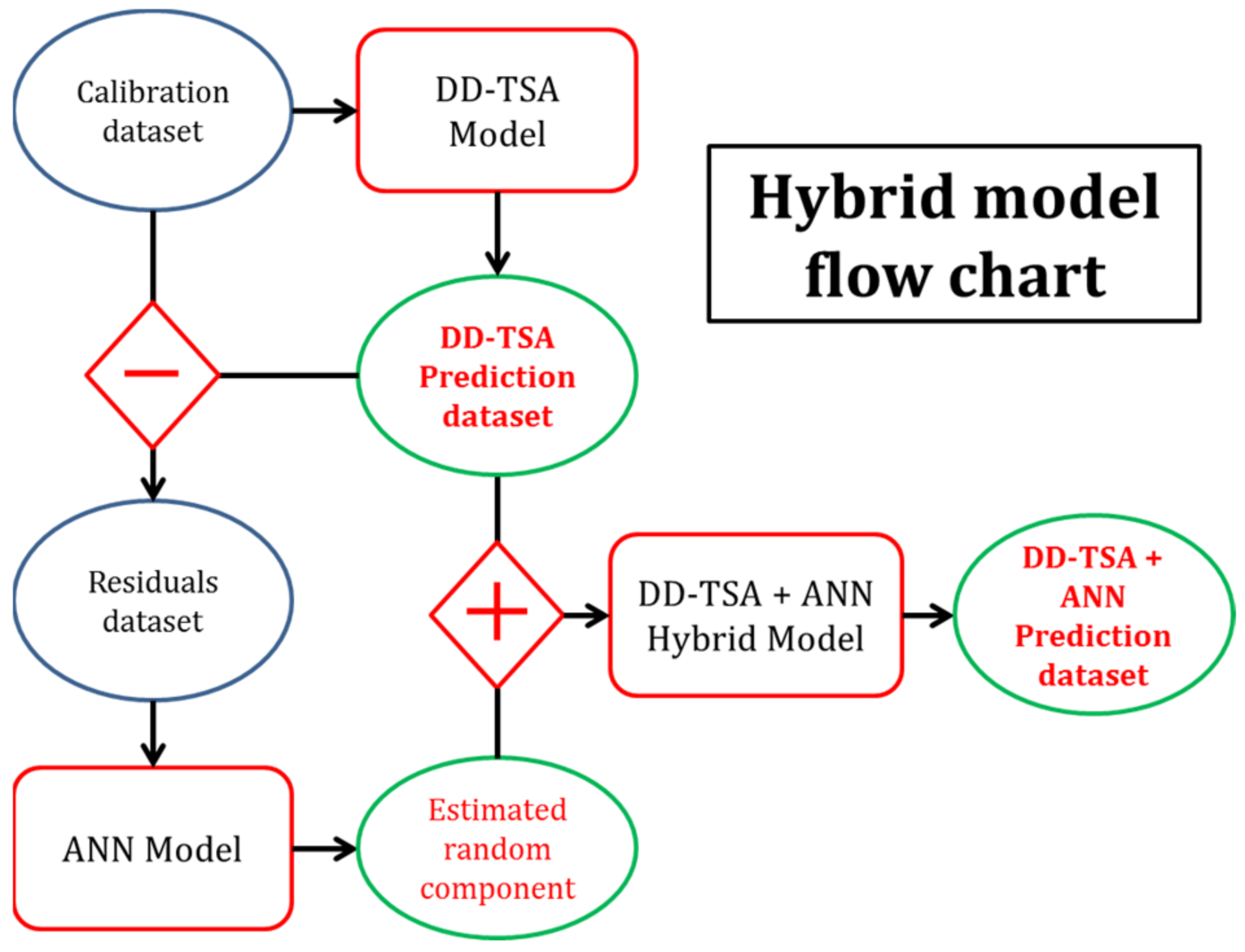
The hybrid procedure presented in this paper is a model made by joining in cascade a Deterministic Decomposition Time Series Analysis (DD-TSA) model and an artificial neural network (ANN). Figure 1 describes the steps of the functioning of the model.
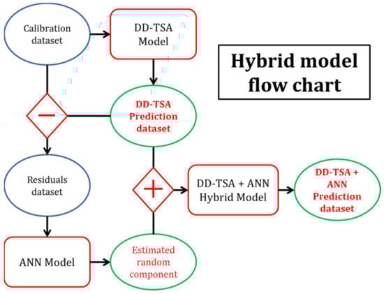
Figure 1.
A flow chart of the hybrid model, composed of the combination of DD-TSA and ANN procedures. The blue circles are datasets, the red squares are the models and the green circles are the output of the different models. Diamond symbols report the algebraic operation between the connected datasets. The schematic visualization describes the passages for obtaining the hybrid model results: at first, the residuals dataset is obtained by subtracting the predicted data from the real one. Such residuals are treated by an ANN that generates the random component. The random component is, upon its turn, added to the predicted values again, to obtain the final hybrid model prediction.
2.1. Time Series Description
The time series used in this work is made of equivalent noise levels (A-weighted) recorded in the city of Messina, Italy, in the proximity of a crowded large road, Viale Boccetta. This road is made of four lanes, two per direction, and is a major connection between the commercial dock and the highway, observing more than 10 million vehicles per year [35]. Due to its position, the recording of the cabinet of Viale Boccetta detects the huge vehicular traffic on the road, and also the contribution of the dock operations, which are minor but not negligible, as described in [36,37]. The measurement station is included in a large network monitoring installed and controlled by the municipality of Messina. This network has been updated recently but, at the time of the measurements used in this application, it was made of 8 monitoring stations distributed along the city, each of them equipped with a class 1 sound level meter Larson & Davis 820 and 831, installed in a waterproof cabinet. Regarding the Viale Boccetta measurement site, the cabinet was installed on the terrace of the first floor of a municipal building that nowadays hosts the “Palacultura” and some of the offices of the municipality. The time basis is one day, i.e., data are equivalent to continuous levels evaluated for 16 h, from 6 a.m. to 10 p.m. The final dataset is made of 1200 LAeq,16 h, split into the first 1100 LAeq,16 h for calibration and the last 100 for validation. Missing data were present, and they were imputed with the same technique used in [38,39]. This operation was necessary because the deterministic decomposition model needs to be calibrated on a continuous dataset since it aims at detecting the seasonality of the data according to the autocorrelation function and the lag.
For model generation, in some analyses, the first 13 data were discarded, resulting in 1087 data left (details will be presented later on). Thus, to evaluate statistical parameters on a common dataset, the comparison dataset in the calibration phase for all the models was reduced to 1087 (from period 14 to period 1100). The statistics of the 1087 data used in the calibration phase are resumed in Table 1: the mean value of 72.54 dBA indicates that the acoustic pollution in the area is very high. Skewness and kurtosis indexes show that the distribution can be considered roughly normal.

Table 1.
A summary of the statistics of the comparison dataset in the calibration phase, 1087 data.
In Table 2, summary statistics of the 100 measured LAeq,16 h between May and August 2010 are shown. The data show that the daily average emission is quite high for this kind of phenomenon, exceeding 71 dBA. Please note that the average acoustic emission measured in these 100 days is not different from that of the 1100 calibration data. The skewness and kurtosis indexes are very close to those characteristics of normally distributed data.
Table 2.
Summary of statistics of 100 performance test datasets.
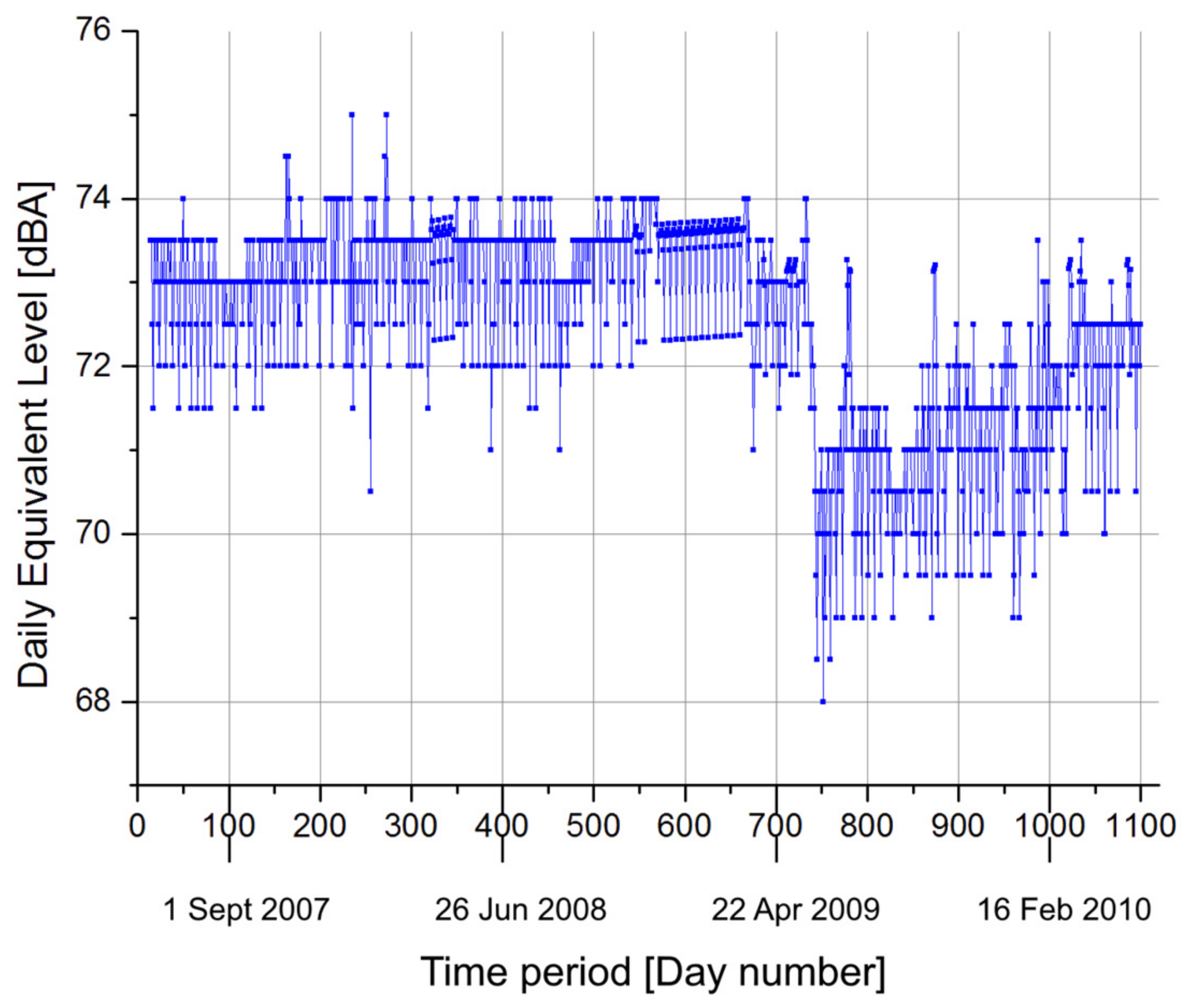
The whole dataset is plotted in Figure 2. The time history of the actual 1087 data used for the comparison in the calibration phase. The related period is between 24 May 2007 and 14 May 2010. It is evident that a drastic change in the mean occurs between periods 730 and 760. Unfortunately, no official information is available about this drop that could be related to many factors, as none of them have scientific evidence supporting it. The authors decided to maintain these data to perform a “non-informative” calibration of the model. Despite this, the overall performances of the model are not affected by this event.
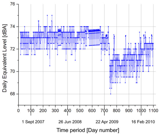
Figure 2.
The time history of the actual 1087 data used for the comparison in the calibration phase. The related period is between 24 May 2007 and 14 May 2010. On the x-axis, timespan is reported, while on the y-axis, LAeq,16 h, expressed in dBA, are present.
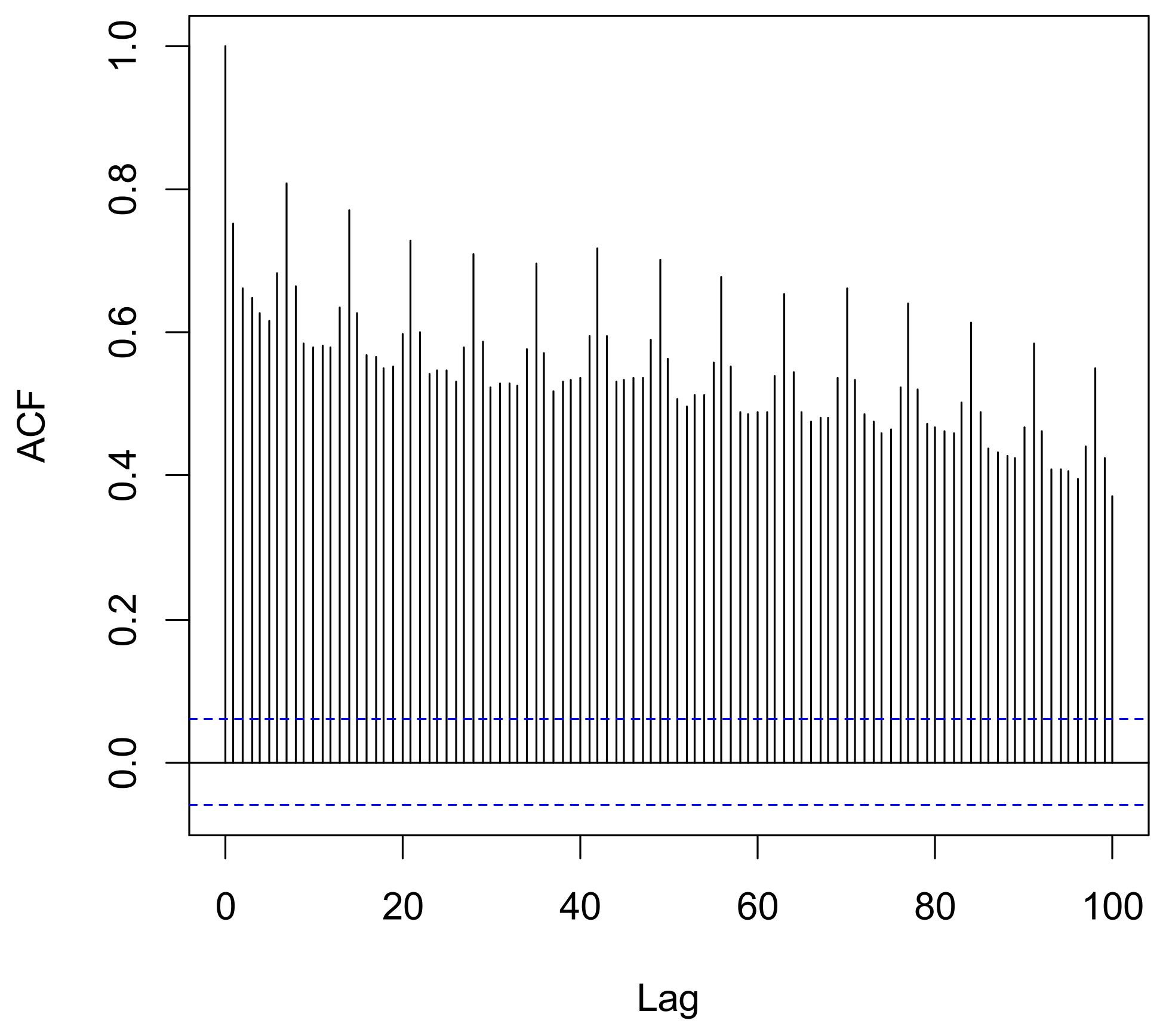
Figure 3 shows the autocorrelation function as a function of the lag. It is evident how the data are correlated and that the higher value of correlation appears at 7 days, suggesting how noise in the measuring location (mainly deriving from road traffic) is influenced by the days of the week. During the weekend, fewer vehicles are in transit, and then the overall noise level is lower. On the contrary, working days are characterized by a higher number of vehicles flowing, with a consequent higher overall noise level.
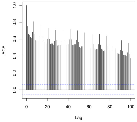
Figure 3.
An autocorrelation plot (correlogram) of the calibration dataset. The alternation of peak autocorrelation for each of the seven lags clearly indicates a weekly correlation between data.
The Augmented Dickey–Fuller (ADF) [33] and Phillips–Perron (PP) [34] tests are proposed and applied to the acoustical data studied in this paper to check the stationarity of the series. In Table 3, the results of the tests are reported: the p-value of the ADF and PP tests does not allow for the rejection of the null hypothesis (presence of unit roots), identifying the series under study as non-stationary. The test results and the good performances of the models here presented indicate the possibility of reproducing the non-linearity and the non-stationarity of the series under study.
Table 3.
Augmented Dickey–Fuller and Phillips–Perron unit root tests for stationarity of time series performed on calibration dataset.
The periodicity of a series can be evaluated with some tests. The Ljung–Box (LB) test [30] looks for autocorrelation of the data and if a fully random data fluctuation must be considered. The results are reported in Table 4, where the small p-values assure that the hypothesis of the absence of autocorrelation in the data can be rejected.
Table 4.
Ljung–Box test performed on calibration dataset.
Other statistical tests can be performed in order to check the linearity in the series under study. The authors in this paper adopt the widely used Lee–White–Granger (LWG) [31] and the Terasvirta–Lin–Granger (TLG) test [32]. For both tests, the null hypothesis to be verified is the linearity of the time series. The results are reported in Table 5, where the very low p-values suggest that the series is non-linear.
Table 5.
Lee–White–Granger (LWG) and Terasvirta–Lin–Granger (TLG) tests for linearity performed on the calibration dataset.
2.2. Deterministic Decomposition Time Series Model
Time Series Analysis (TSA) is commonly performed by analyzing the time series both in time and frequency. In the time domain, the more interesting features are the time slope, the ratio of past/present, the memory of the series, the autocorrelation of the data, etc. On the other hand, in the frequency domain, the aim is to decompose the time series into its fundamental periodic components, each of them characterizing the signal and representing a seasonal behavior. Time series have different components: the trend represents the long-term behavior of the data and can be detected with regressive methods. Seasonality is the short-term periodicity, the repetition of a given phenomenon that cyclically affects the data and can be pointed out with autocorrelation studies and lag detection. Finally, the random component represents the non-deterministic part of the series, the unpredictable feature of the physical phenomenon.
At is the actual data measured in a period t, and Dt is the multiplication of trend and seasonality. The random component et represents any casual variation from the trend and the seasonality of the time series that cannot be predicted a priori with any deterministic formula. For these reasons, the latter component can be only “estimated” but not “predicted”. The Deterministic Decomposition Time Series Analysis model (DD-TSA) here presented in this paper is aimed at the prediction of the deterministic part of the series, i.e., trend and seasonality, with the following formula:
where b0 is the intercept, b1 is the slope of the trend line and is the seasonal coefficient. To visualize the trend, a linear regression on the calibration dataset and the seasonal coefficient is performed, according to what the authors reported in [40]. The parameters of the calibration are reported in Table 6 and Table 7.
Table 6.
Model parameters estimated on the calibration dataset: b0 is the intercept, where b1 is the slope of the trend line.
Table 7.
Model parameters estimated on the calibration dataset: are the seasonal coefficients referring to the the seven days.
Given the output of this model, the residuals can be calculated as the difference between the actual data and the DD-TSA output:
The of the DD-TSA process are used to train an artificial neural network (ANN). In particular, the neural network here implemented is a feedforward backpropagation network: it is a multilayer perceptron model largely adopted and documented in the literature. The network was developed in the Matlab R-2018 framework, using the Neural Network 2019b Tool.
2.3. Artificial Neural Network Model
ANNs are a type of model made by the union of simple mathematical functions acting in a parallel structure, able to simulate the behavior of the human brain. These functions are called “artificial neurons”; they have many inputs, with assigned weights, and a single output. The activation of the single neuron is a function of the weighted mean of inputs. This structure is able to learn and generalize, producing outputs even with unknown inputs. The simplest way to train an ANN is to give as input a series of data (training set) and to compare the response of the network with the true value. Once the difference between the two responses (error) is evaluated, the weights can be adjusted to minimize the error or to bring the error below a given threshold.
The ANN implemented in this paper is a feedforward backpropagation network trained with the “trainlm” function of Matlab, which optimizes the error estimation through the Levenberg–Marquardt optimization. The adaptation learning function is the “learngdm” one, which is the gradient descent with momentum weight and bias learning functions. The model has seven inputs and a single output, i.e., , which represents the error of the network at the period t. The hidden layer is single and is made of 140 neurons, i.e., 20 times the inputs. The transfer function for the hidden layer neurons is of the sigmoid type, while the one for the output neurons is linear.
The objective function to minimize is the mean squared normalized error performance function, and the learning algorithm stops at the value of 0.01. The adopted strategy to improve the generalization performances of the network and to reduce overfitting risks is the “Cross-validation”. The maximum number of accepted worsening in the validation phase, before the algorithm stops, is 10.
Once the weights have been calculated, the ANN can give an output for the estimation of the random component . For the purposes of the present work, two different neural networks have been designed and implemented, with different input vectors and, consequently, different prediction horizons: ANN (t-1) and ANN (t-7).
The used dataset is divided into three parts: one for the training of the network (60%), one for the validation (20%) and one for the test (20%). Two cycles of training were executed, to obtain an optimum minimization of the objective function.
2.3.1. ANN (t-1) Model
The ANN (t-1) model takes in as input seven residuals produced by the DD-TSA application, prior to the one to be predicted. The single output of this feedforward neural network, , represents the estimation of the stochastic term in Formula (1) that is used to implement the hybrid model. The structure of the ANN is summarized in Table 8.
Table 8.
The topological structure of the ANN (t-1) model.
The dataset adopted to train the network is divided into three parts, one for the training (60% of the 1100 data), one for the validation and one for the test, which are both 20% of the entire dataset. Two cycles of training were executed, to obtain an optimum minimization of the objective function.
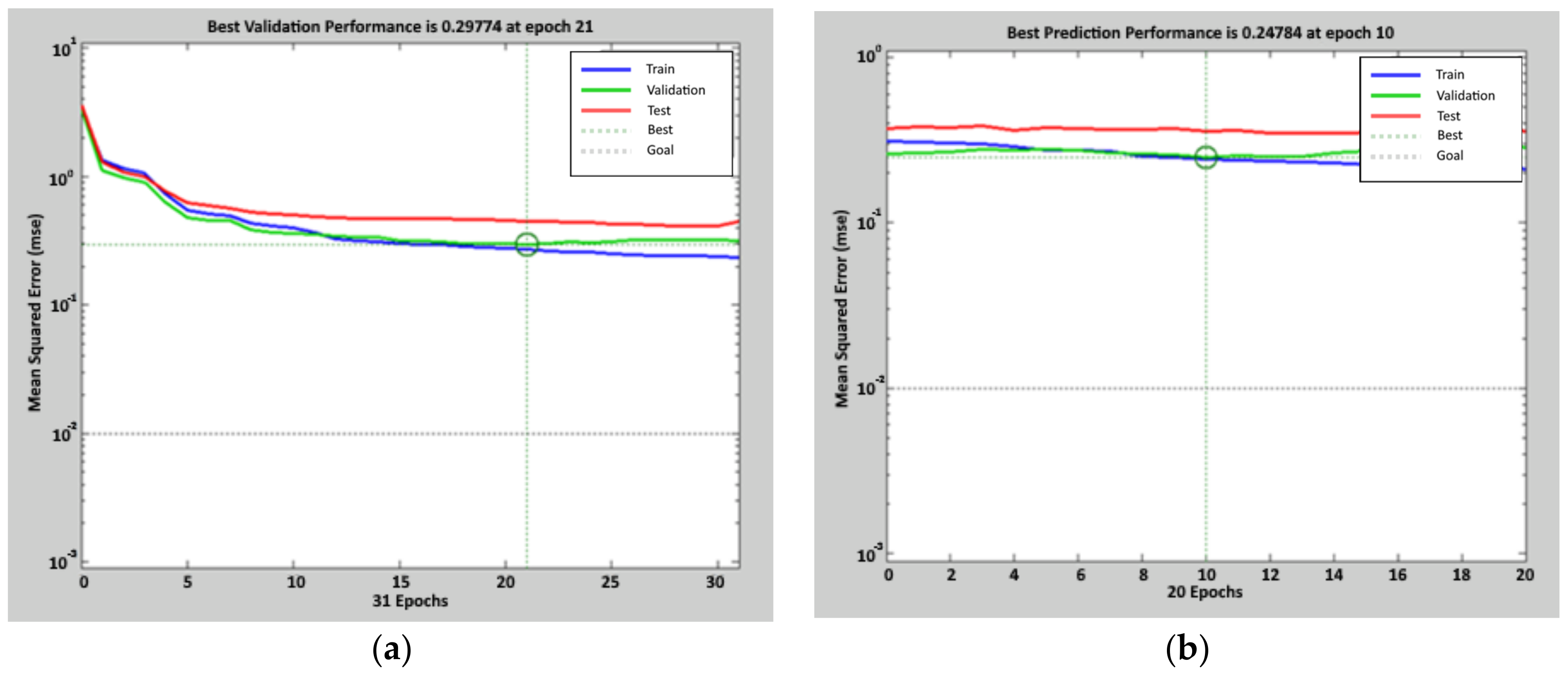
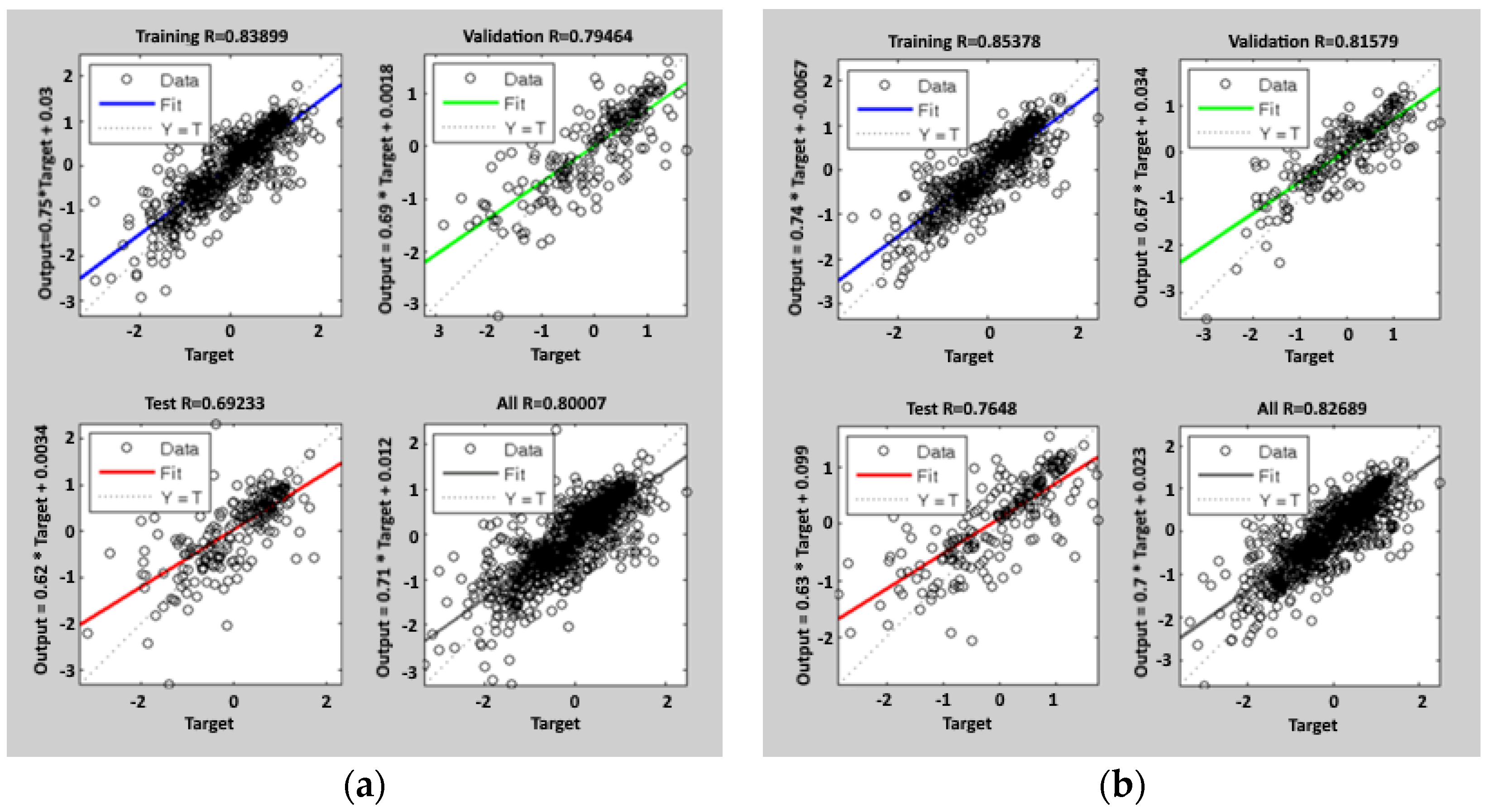
The results are shown in Figure 4: the lower value of the objective function, in the validation data, is 0.30 for the first cycle and 0.25 for the second one. This result was achieved after 21 epochs on the first cycle and after 31 epochs on the second cycle. In Figure 5, regression lines are reported, with related functions, obtained comparing target data with the ones predicted by the network during the training in the two cycles: the correlation coefficient R, obtained considering the entire set of 1100 data of calibration, is 0.80 at the end of the first cycle and 0.82 at the end of the second cycle.
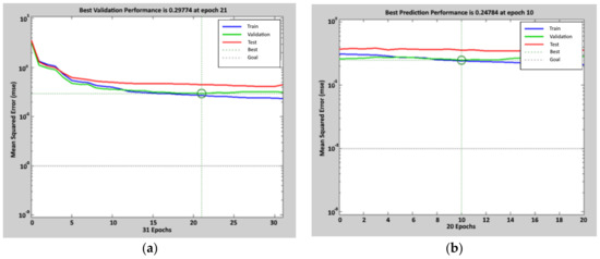
Figure 4.
Performance achieved during the calibration process of the ANN (t-1) model. For the first tuning, the figure on the left (a), the mean square error after 21 epochs is 0.30. For the second tuning, the figure on the right (b), the mean square error after 10 epochs is 0.25. Circles indicate the values at the selected epoch.
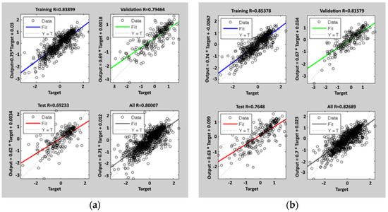
Figure 5.
Regression lines after the training process of the ANN (t-1) model: the blue line is the fit on 60% of the training data, the green line is the fit on 20% of the validation data, and the red line is the fit on 20% of the test data. The dashed line is the bisector of the plot, where simulated data are equal to the real ones. The last plot is the regression fit on all 1087 data; the figure on the left (a) is related to the first tuning, and the figure on the right (b) is related to the second tuning.
The network adopted in the following predictive application is the one with the weights calculated during the second cycle of training.
2.3.2. ANN (t-7) Model
The ANN (t-7) model is very similar to the ANN (t-1), except for the input vector. In this case, the 7 input residuals, , are not close to the one to be predicted but are shifted seven days backward. In this way, by moving the input vector from t-13 to t-7, this model can give an output of seven predictions, from t to t+6. The structure of the network is reported in Table 9.
Table 9.
Topological structure of ANN (t-7) second neural network.
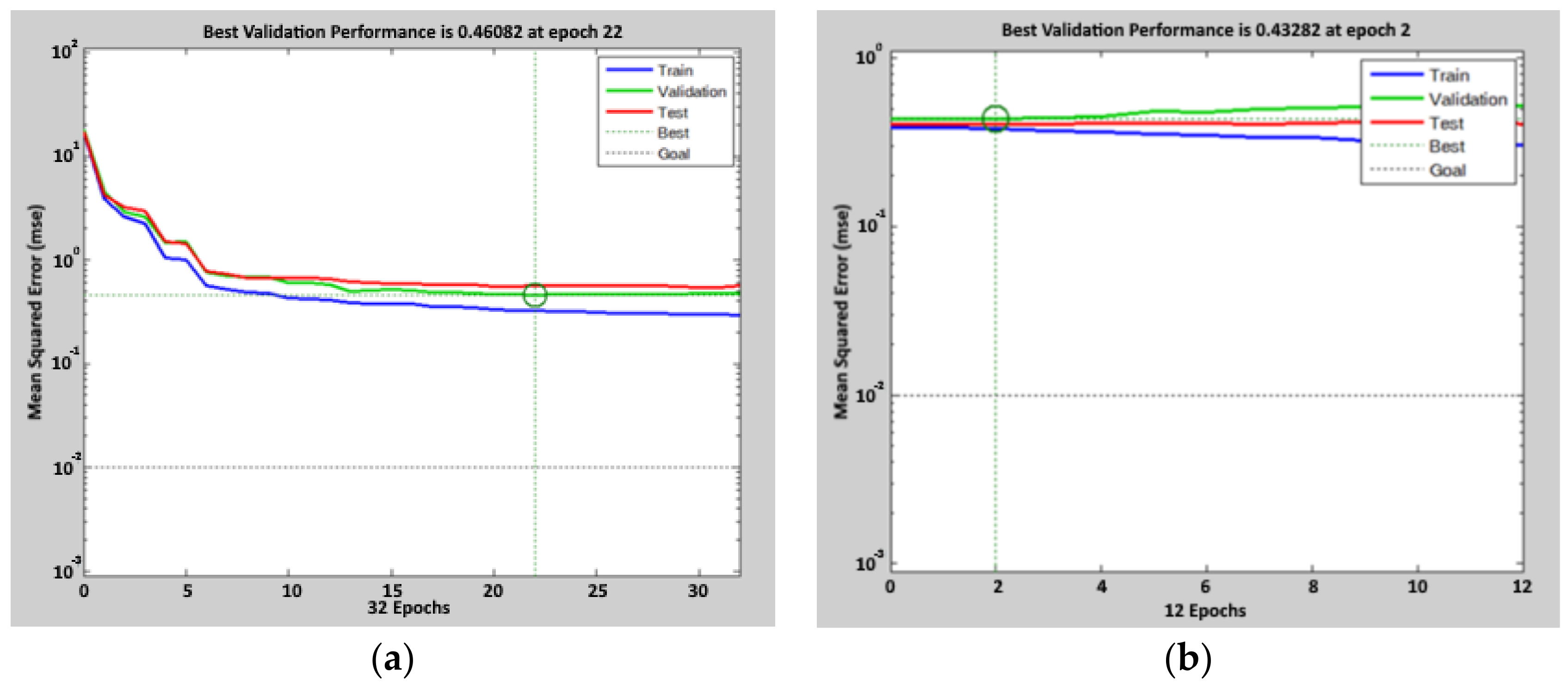
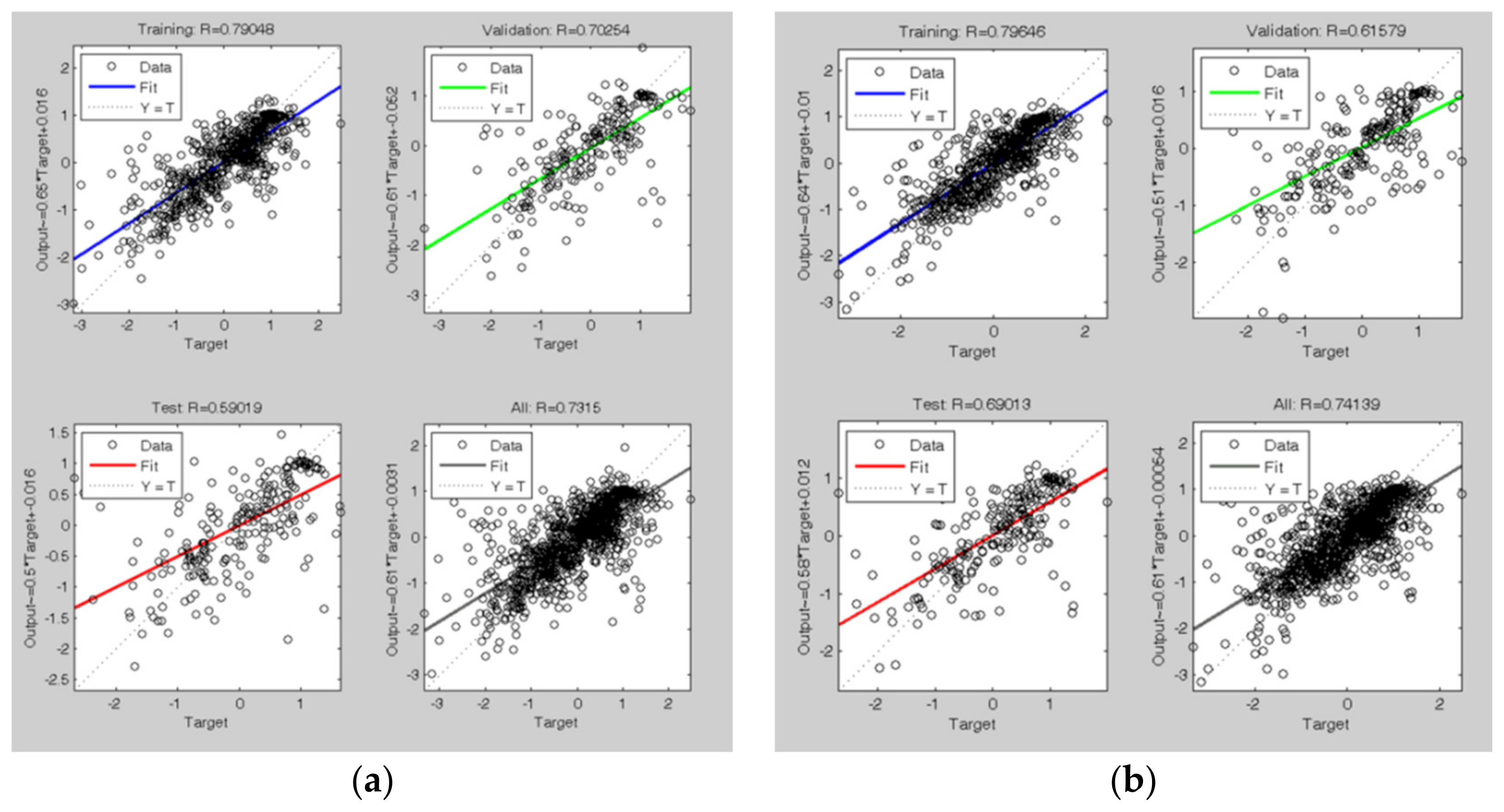
Again, two cycles were run, to minimize the objective function. In Figure 6, the results of the two training cycles are reported: the lowest value for the objective function is 0.46 for the first cycle and 0.43 for the second one. These results were achieved after 22 epochs in the first cycle and after 24 epochs in the second cycle. In Figure 7, the regression lines are shown: the correlation coefficient is 0.73 at the end of the first cycle and 0.74 after the second one. Thus, thanks to the weekly periodicity of the dataset, the network still has good predictive performances, even if the input vector includes data that are “one week old” compared to the considered day.
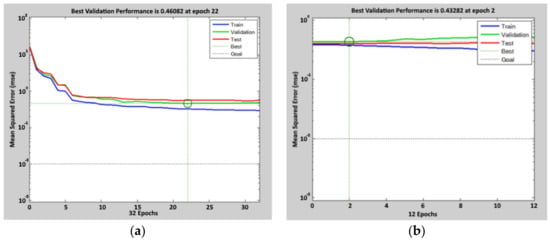
Figure 6.
Performance achieved during the calibration process of the ANN (t-7) model. For the first tuning, the figure on the left (a), the mean square error after 22 epochs is 0.46. For the second tuning, the figure on the right (b), the mean square error after 2 epochs is 0.43. Circles indicate the values at the selected epoch.

Figure 7.
Regression lines after the training process of the ANN (t-7) model: the blue line is the fit on 60% of the training data, the green line is the fit on 20% of the validation data, and the red line is the fit on 20% of the test data. The dashed line is the bisector of the plot, where simulated data are equal to the real ones. The last plot is the regression fit on all 1087 data; the figure on the left (a) is relative to the first tuning, and the figure on the right (b) is relative to the second tuning.
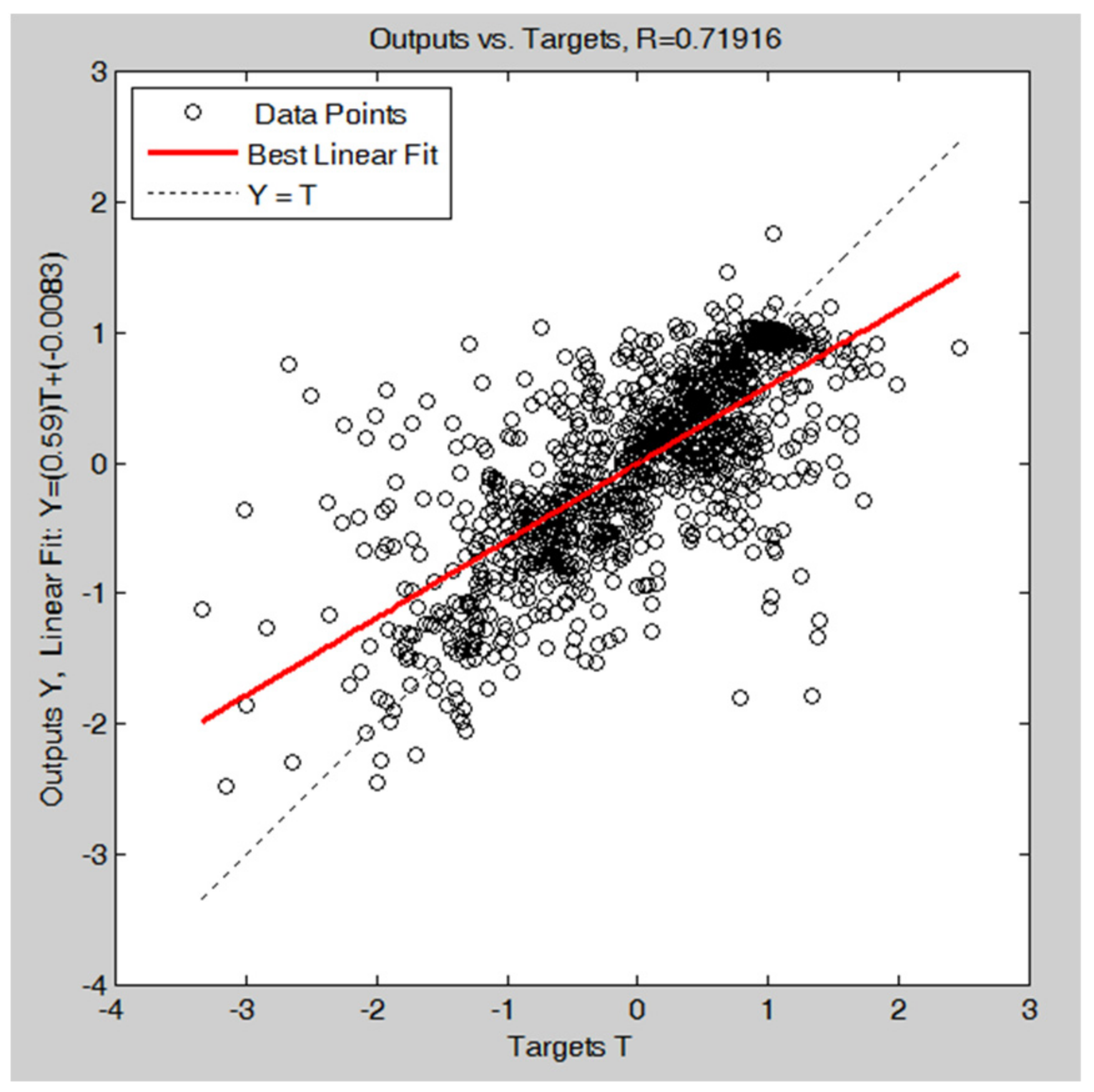
The set of weights obtained with the second training cycle has been used in the network to be combined with the DD-TSA model for prediction. Figure 8 shows the predicting results of the trained network, in the set of 1087 data used in the calibration phase: in this case, the good forecasting performances are confirmed by a correlation coefficient of 0.72.

Figure 8.
Regression fitting of the ANN (t-7) model after the network simulation on the calibration data. The plot is relative to the second tuning.
The prediction of the final hybrid model is given by the following:
in which is the DD-TSA output (deterministic part prediction) and is the ANN output (random component estimation). The error of this model (or residual if calculated in the calibration phase) is given by the following:
This error will be used to check the performance of the different models and to highlight their peculiarities.
3. Results
After the previous calibration phase, in which all parameters, coefficients and weights of the network were estimated, it is possible to input into the hybrid model the noise emissions of previous periods and the forecasting errors generated by the DD-TSA model: in this way, it is possible to have, as the output, the predictions of LAeq,16 h for future days.
In the performance test phase, the LAeq,16 h, and the errors generated during DD-TSA forecasts from period 1101 to 1200 (15 May 2010 to 22 August 2010) were used.
As stated before, these data were not used to calibrate the coefficients and parameters of the DD-TSA model or to update the weights of the ANN, so they constitute an effective dataset to evaluate the real predictive power of the developed hybrid model. In this article, the authors have adopted two error metrics: mean percentage error (MPE) and the Coefficient of Variation of the Error (CVE).
Once the three models (DD-TSA, DD+ANN (t-1) and DD+ANN (t-7)) have been calibrated, a detailed comparison can be pursued. In this section, the comparison is performed qualitatively, with a plot of the model predictions and of the actual values, and quantitatively using residual distributions analysis and error metrics (MPE and CVE).
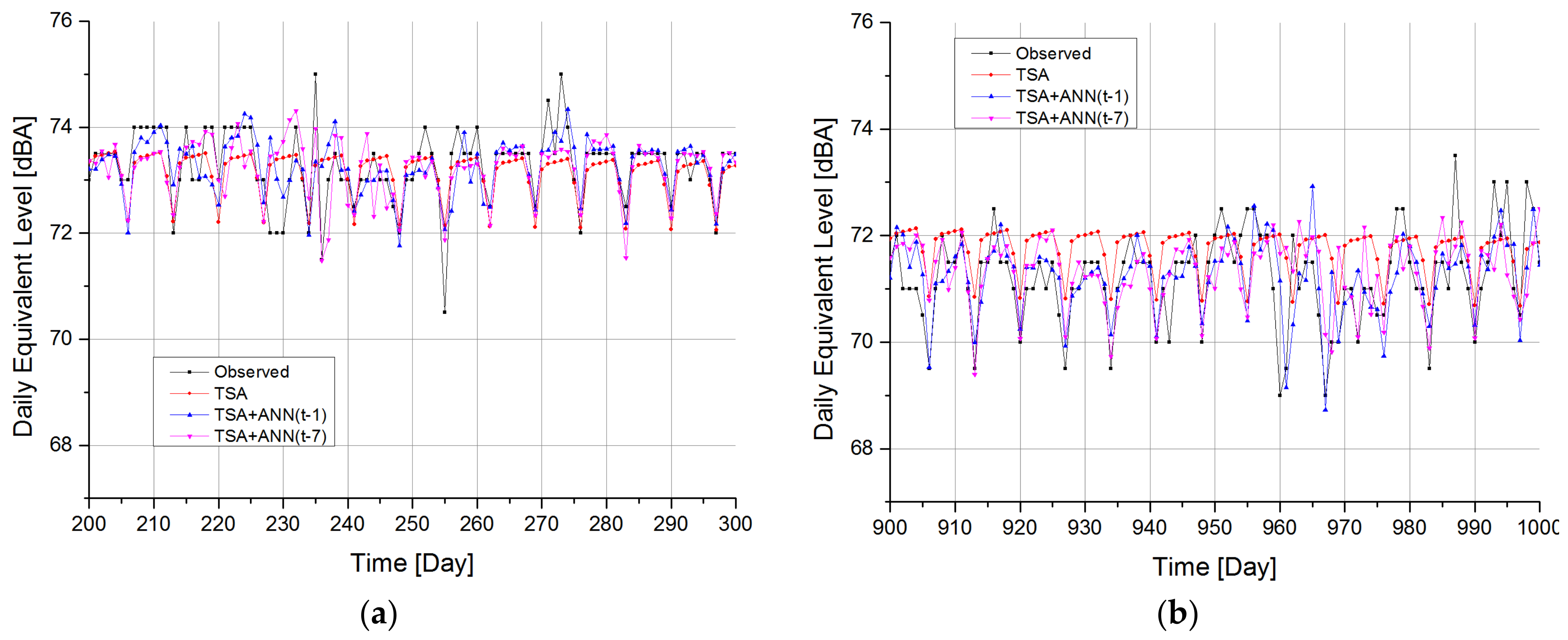
Figure 9 reports the actual and predicted time series in two different intervals of the entire range under study. All the models follow the general slope of the data, with moderate agreement.
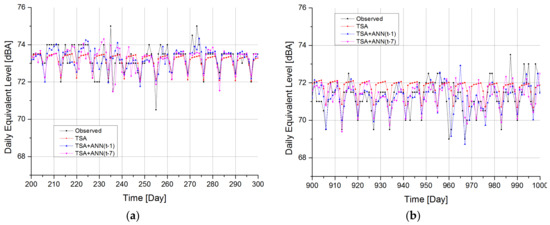
Figure 9.
Time history comparison between real data DD-TSA, DD+ANN (t-1) and DD+ANN (t-7) predictions. In (a), data are shown from 26 November 2007 to 5 May 2008. In (b), the period between 26 October 2009 and 3 February 2010 is reported.
As for the quantitative comparison, the “overall” residuals of the models can be evaluated by looking at the difference between observed and predicted values. In particular, for the DD-TSA model, is computed as in Formula (3), whereas the hybrid models are computed as in Formula (5).
In Table 10, the statistics of the residuals of all the models are presented. The mean value of the residuals is basically negligible for all three models. The two hybrid models exhibit a lower standard deviation compared to the DD-TSA model, suggesting a lower dispersion of the error.
Table 10.
Residual statistics resume for the 1087 comparison Leq16 h in the calibration phase.
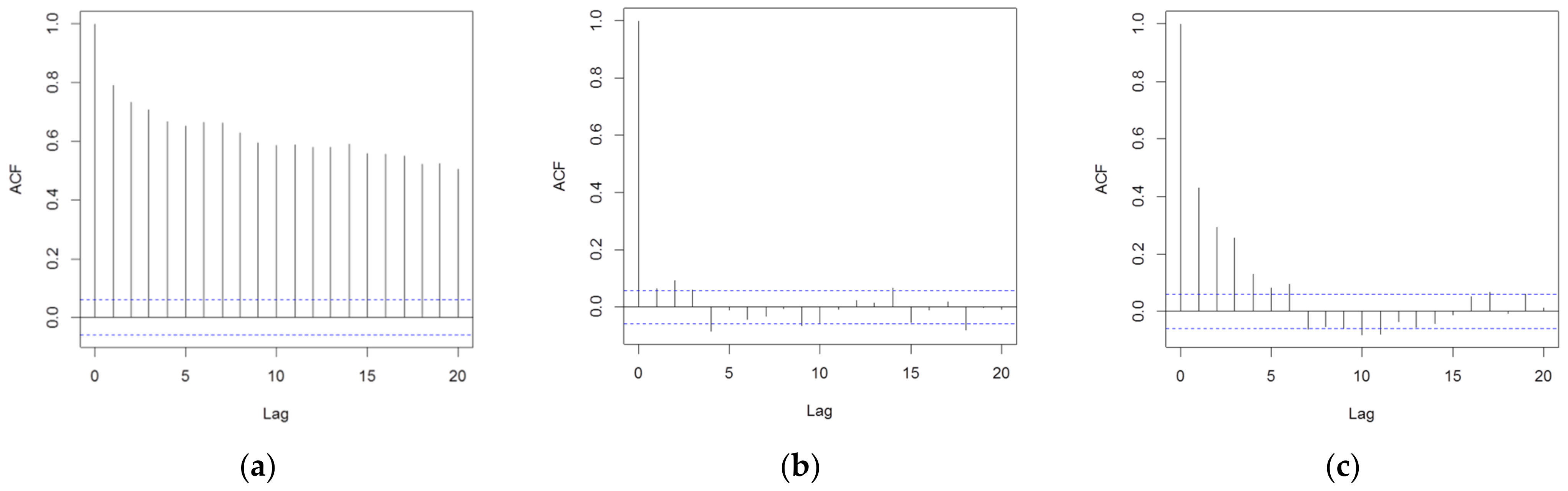
Residual autocorrelation has been tested with an autocorrelation plot (Figure 10). A very high correlation is detected in the DD-TSA residuals dataset. This means a lot of information in this series is present that the neural network can use to improve the prediction. Looking at the hybrid models, both exhibit a much lower autocorrelation compared to the DD-TSA model, for any value of lag. In particular, the DD+ANN (t-1) model seems to be able to better explain the variance in the data, since it quite completely removes the autocorrelation in the residuals. On the contrary, the residuals dataset of the DD+ANN (t-7) still shows a non-negligible autocorrelation, especially for values of the lag up to 6. This was expected since this model uses the 6 closer data to provide the forecast.
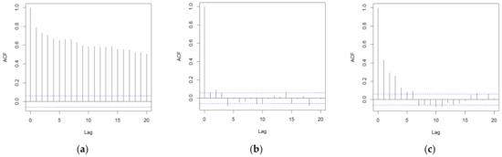
Figure 10.
Correlogram plot for the residuals, evaluated in the comparison dataset of the calibration phase (1087 data): on the left, (a) the DD-TSA model, in the center, (b) the DD+ANN (t-1) model, and on the right, (c) the DD+ANN (t-7) model. The value of the autocorrelation coefficient is plotted as a function of the lag. Blue dotted lines represent the threshold of 0.1, under which the data are considered not autocorrelated.
In Table 11, the values of the autocorrelation function computed for 7- and 14-day lags are presented. It is easy to notice the very low level of autocorrelation in the residuals dataset of the two hybrid models.
Table 11.
Values of the autocorrelation function in the residual calibration dataset. The function is evaluated for two representative lags: 7 and 14 days.
In Table 12, MPE and CVE results are reported, indicating the good provisional capability of the DD-TSA model in terms of mean percentage error. Despite the analyzed series being non-stationary due to the abrupt change in mean during the periods from 730 to 760, all three models can provide forecasts not affected by high distortions: the achieved forecasts on average do not overestimate or underestimate the actual data. The CVE metric shows that the best model in terms of low residual dispersion is the DD+ANN (t-1).
Table 12.
MPE and CVE values for DD-TSA, DD+TSA (t-1) and DD6+TSA (t-7).
Time History Plot Comparison and Forecast Errors Analysis
Analysis of the error of the three proposed models gives information on attitudes of the three strategies to forecast LAeq,16 h in periods not used in the calibration phase. In Figure 11a, it is easy to see that the DD-TSA model underestimates the real value of acoustic emission in every 100 periods of the performance test. To correct this wrong behavior, it may be advisable to recalculate the trend by cutting part of the oldest periods of the calibration series. The weekly periodicity of the series is reproduced with good approximation, but some emission peaks are not adequately predicted by the model because of the completely random nature of these events.
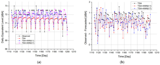
Figure 11.
Time history (a) and error (b) comparison between observed data and model results in performance test dataset, i.e., between 28 May 2010 and 22 August 2010.
In particular, an unexpected low LAeq,16 h is observed in period 1119: this event is not predicted by any of the three models. This low LAeq,16 h is observed during a national Italian holiday called “celebration of the Republic”. In the following time interval, in which there is a gradual recovery of normal traffic, the emission level also increases, but it is still lower than the average of the period. In this case, the DD+ANN model (t-1), being the fastest to follow the sudden and unexpected changes, manages to resemble the actual observed data. The effect of reduction due to the low value observed during June 2 in the LAeq,16 h foreseen by the DD + ANN model (t-7) occurs only after seven periods, with a negative result on the error of prediction of the model at that time period. In general, to solve the problem of forecasting during public holidays, it would be appropriate to include in the neural network a “flag” type input to distinguish working days from holiday periods. In Figure 11b, the forecasting errors provided by the three models in the 100 periods of the performance test are shown. In particular, the errors of the DD-TSA model were evaluated according to Formula (3), while the errors of the two hybrid models with ANNs in cascade have been calculated according to Formula (5). It can be noticed that the errors of the DD-TSA model are not random but still exhibit a weekly periodicity which was not adequately reproduced by the model. In addition, most of the errors are positive, further confirming that the model underestimates the measured data during this time interval. The plots of hybrid models show a greater dispersion around zero but are nevertheless distributed more evenly between positive and negative values.
Table 13 shows the statistics of the model errors on 100 periods of the performance test. The mean and median of the error for the DD−TSA model are different from zero, due to the underestimation compared to the observed data. On the contrary, for hybrid models, both the mean and the median are very low and close to zero.
Table 13.
Error statistics resume for the 100 performance test periods.
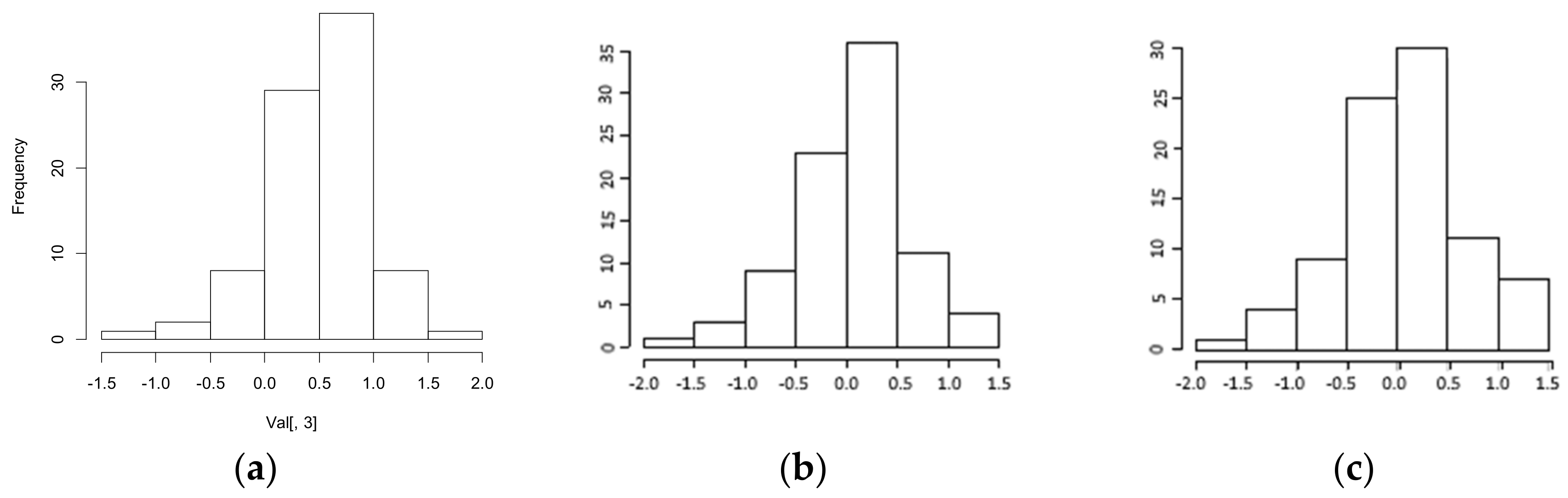
The normal distribution of the errors is a plausible hypothesis for the two hybrid models: the kurtosis and symmetry indices deviate insignificantly from zero. The assumption of normality of the errors can also be positively evaluated thanks to the histograms shown in Figure 12.
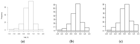
Figure 12.
(a) A histogram of the errors of the DD-TSA model. (b) A histogram of the errors of the DD+ANN (t-1) model. (c) A histogram of the errors of the DD+ANN (t-7) model. All of them were tested on 100 performance test days.
In addition, also the results of the Jarque–Bera test, shown in Table 14, do not allow for the rejection of the normal distribution assumption of errors for the two hybrid models.
Table 14.
Jarque–Bera normality test performed for the errors of the three models applied to the 100 performance test data.
The normal distribution assumption of errors for the DD-TSA model is less strong but must not be abandoned, as shown by both the kurtosis and symmetry indices not being excessively high.
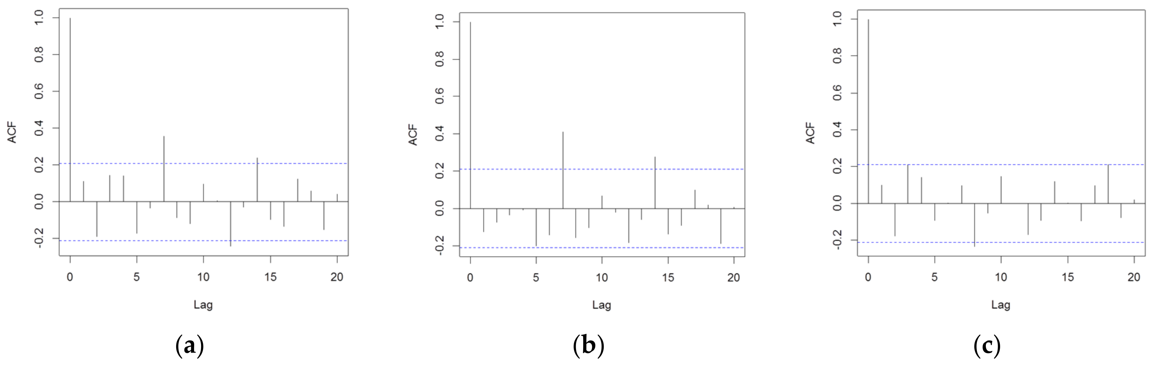
The behavior of the error autocorrelation function during the performance test phase has been evaluated. If the error dataset still contains high residual autocorrelation, the adopted models were probably not able to extract all the information content due to temporal dependencies in the series.
In Figure 13, it can be noted that both the DD-TSA model and the DD+ANN (t-1) model forecast errors have a weekly autocorrelation (a lag equal to 7) that is statistically significant. However, this autocorrelation is much lower compared to that present in the original series for the same lag, which was equal to about 0.7. However, the DD+ANN (t 7) model has shown to have no significant residual autocorrelation in the dataset of forecast errors. Even the values of the autocorrelation error function for important lags, such as 7 and 14 periods, are very low, as shown in Table 15.
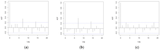
Figure 13.
A correlogram of the errors for (a) the DD-TSA model, (b) the DD+ANN (t-1) model and (c) the DD+ANN (t-7) model, evaluated in the performance test phase (100 data). On the x-axis, lag is reported, and on the y-axis is the autocorrelation function.
Table 15.
The values of the autocorrelation function in the error performance test dataset. The function is evaluated for two representative lags: 7 and 14 days.
The MPE and CVE results of Table 16 indicate the good performance of the two hybrid models in terms of prediction distortion. Also, the error dispersion of the two models with ANNs in cascade is very low.
Table 16.
MPE and CVE of two different models.
On the other hand, the high value of the MPE index for the DD-TSA model shows that, by using this procedure and this calibration dataset, it failed to grasp the behavior of the performance test series and it provided an underestimation of the prediction of the observed real data.
4. Conclusions
In this paper, a time series composed by LAeq,16 h coming from measurements in the city of Messina (Italy) has been thoroughly analyzed. The dominant noise source is road traffic, together with anthropogenic noise mainly due to the commercial port nearby. Other components, even if they are a minority, cannot be excluded. The classical prediction techniques for the noise produced by human activities need the knowledge of many variables, such as, for instance, the number of transiting vehicles, average speed and the type of vehicles. In this study, the authors show that, if the acoustic emission is strongly related to regular activities, the environmental noise level also exhibits a periodic pattern. If this regularity is observed and detected, it is possible to compute an accurate forecast of LAeq,16 h, having, as the input, only measured LAeq,16 h over a sufficiently large time interval.
In the case study analyzed in this paper, the time series is highly self-correlated and non-linear. The series also shows a non-stationary pattern, since an abrupt change in the mean value is noticeable. The LAeq,16 h prediction is made by three different models, which have been calibrated using the set of 1100 measurements, and their forecast performances on a performance test dataset of 100 measurements, not used in the calibration, have been studied.
One of the models has been built with a classical decomposition technique (DD-TSA), which exploits the periodic pattern and the trend of the series. The residuals of the DD-TSA model application in the calibration dataset have been used as input for two feedforward neural networks (ANNs), which estimate the stochastic component of the series. In this way, two hybrid models have been built, combining in cascade the prediction of the DD-TSA and the ANN models. In particular, the two hybrid models differ from the range of the forecast, which is one step ahead for the DD+ANN (t-1) model and seven periods ahead for the DD+ANN (t-1) one.
In the calibration phase, all the models were able to capture the periodic pattern of the series and the general trend, with low means and standard deviations of the residual distribution. Nevertheless, the hybrid models provided a very good prediction, reasonably removing all the residual autocorrelation.
After the calibration of parameters using the 1100 first observation of the series, the three models have been used to forecast the last 100 LAeq,16 h from day 1101 to day 1200. Good predictive performances are shown by the three proposed models. In particular, the model DD-TSA, characterized by the largest forecast horizon, shows a higher error in the predictive phase.
It is noteworthy to consider that, in the calibration phase, all the available data were considered and used, even if a sudden drop in the mean level, interrupting the stationarity of the time series, was present. In this way, the authors performed a “non-informative” calibration of the model itself, which resulted in very good provisional properties. Even if such a sudden drop in the noise level was due to malfunctioning or accidental events, the hybrid model preserves its good provisional capability when calibrated with those data.
A substantial improvement in the error statistics, normality and autocorrelation is obtained with the two hybrid models, even though this new technique is characterized by a short forecast horizon. The forecast errors provided by the hybrid models, with respect to the ones obtained with the DD-TSA model, show a lower mean value (but a slightly higher standard deviation), a normal distribution and, in the case of the DD+ANN (t-7) model, a lower autocorrelation for the 7 and 14 lags.
The limitations of this study are mainly related to the need for a large and non-biased dataset to calibrate the models, to tune the hyperparameters and the parameters of the selected approach and to provide reliable forecasts. The strength of such models, in fact, is that they use input only past measurements of the acoustic descriptor to be predicted, in our case, the daily LAeq,16 h. It does not require any information about traffic flows, traffic composition, average speed, etc., as the standard Road Traffic Noise Models (RTNMs). Of course, this makes the model very sensible to the quality of the input data. From a practical point of view, the authors do not believe this model could be easily and directly used for the commonly used procedure for strategic noise mapping of an urban area. The amount of data required for such a procedure, in fact, does not match with the essential nature of the here presented model, which deals with one single input. On the other hand, our model can be useful to validate any kind of mitigation actions designed and predicted with the very same tools involved in the noise mapping procedures. Any time a strong action on the traffic road framework is implemented, in fact, a new acoustic scenario is born. While its prediction requires many different types of data and a more complex computational framework, the acoustic changes deriving from it could be included in the model with a new calibration, which would certainly modify the model parameters values and adapt to the new conditions. This feature highlights how the model is suitable to be used wherever an unattended long-term measurement station is installed since this kind of instrument provides a time series of noise levels that are perfect for the model calibration. The availability of continuous measurements, in fact, allows for the performance of new calibrations when the model results start to deviate from the observed data.
Another limitation of the hybrid models is the short forecast range, compared to the DD-TSA model. The “one step ahead” prediction made with the DD+ANN (t-1) model appears to be more precise but may be too short for urban planning purposes. The DD+ANN (t-7) model seems to be the best compromise, offering a one-week prediction range with a low predictive error.
Future steps of this research will be the calculation of the trend of the time series considering only a short time interval, not far from the periods in which the forecast is computed, in order to avoid the effect of strong changes in the series mean. In addition, a further evolution of this technique can be the construction of a new hybrid model using a preliminary ARIMA linear model followed in cascade by a recurrent neural network (for instance Hopfield network). Finally, a more detailed hyperparameter tuning of the ANN part of the model will be carried out, to try and reach even more precise forecasting performances of the hybrid model.
Author Contributions
C.G. conceived and designed the experiments; D.R. built the models; D.R., D.S. and C.G. analyzed the data; and D.R., D.S. and C.G. wrote the paper. All authors have read and agreed to the published version of the manuscript.
Funding
This research received no external funding.
Institutional Review Board Statement
Not applicable.
Informed Consent Statement
Not applicable.
Data Availability Statement
Restrictions apply to the availability of these data. Data were obtained from Municipality of Messina and are available at https://amministrazione-trasparente.comune.messina.it (accessed on 18 August 2024), with the permission of Municipality of Messina.
Acknowledgments
The authors are grateful to the local government of Messina, for making the long-term noise levels measured in the city available. The authors dedicate this paper to the loving memory of Carmine Tepedino who passed away in 2017. Carmine partially worked on this model during his PhD research. The will to conclude the work started by Carmine some years ago led us to complete the models and finalize the results presented in this manuscript.
Conflicts of Interest
The authors declare no conflicts of interest.
References
- Growth, U. Green cities. In Escaping Nature; Duke University Press: Durham, NC, USA, 1996; Volume 13. [Google Scholar] [CrossRef]
- Berglund, B.; Lindvall, T.; Schwela, D. Guidelines for Community Noise; Noise & Vibration Worldwide; World Health Organization: Geneva, Switzerland, 1995; Volume 31, pp. 1–141. Available online: http://multi-science.metapress.com/openurl.asp?genre=article&id=doi:10.1260/0957456001497535 (accessed on 23 January 2024).
- Fiedler, P.E.K.; Zannin, P.H.T. Evaluation of noise pollution in urban traffic hubs-Noise maps and measurements. Environ. Impact Assess. Rev. 2015, 51, 1–9. [Google Scholar] [CrossRef]
- Tian, Z.; Feng, T.; Timmermans, H.J.P.; Yao, B. Using autonomous vehicles or shared cars? Results of a stated choice experiment. Transp. Res. Part C Emerg. Technol. 2021, 128, 103117. [Google Scholar] [CrossRef]
- Yadav, A.; Mandhani, J.; Parida, M.; Kumar, B. Modelling of traffic noise in the vicinity of urban road intersections. Transp. Res. Part D Transp. Environ. 2022, 112, 103474. [Google Scholar] [CrossRef]
- Singh, D.; Francavilla, A.B.; Mancini, S.; Guarnaccia, C. Application of machine learning to include honking effect in vehicular traffic noise prediction. Appl. Sci. 2021, 11, 6030. [Google Scholar] [CrossRef]
- European Environment Agency. Environmental Noise in Europe—2020; no. 22/2019; European Environment Agency: Copenhagen, Denmark, 2020. [Google Scholar]
- World Health Organization. Burden of Disease from Environmental Noise; World Health Organization: Geneva, Switzerland, 2011; p. 128. [Google Scholar]
- European Commission. Directive 2002/49/EC Relating to the Assessment and Management of Environmental Noise; FAO: Rome, Italy, 2002. [Google Scholar]
- Klami, T.; Blesvik, T.; Olafsen, S. Long term measurements of highway traffic noise, no. 0218, 2017. Available online: https://admin.artegis.com/urlhost/artegis/customers/1571/.lwtemplates/layout/default/events_public/12612/Papers/2025892_Klami_BNAM18.pdf (accessed on 18 August 2024).
- Gauvreau, B. Long-term experimental database for environmental acoustics. Appl. Acoust. 2013, 74, 958–967. [Google Scholar] [CrossRef]
- Dobrilović, D.; Brtka, V.; Jotanović, G.; Stojanov, Ž.; Jauševac, G.; Malić, M. The urban traffic noise monitoring system based on LoRaWAN technology. Wirel. Networks 2022, 28, 441–458. [Google Scholar] [CrossRef]
- Ascari, E.; Cerchiai, M.; Fredianelli, L.; Licitra, G. Statistical Pass-By for Unattended Road Traffic Noise Measurement in an Urban Environment. Sensors 2022, 22, 8767. [Google Scholar] [CrossRef]
- Wayson, L.; Ogle, T.W.A. Development of Reference Energy Mean Noise in Florida. Transp. Res. Rec. 1993, 82. [Google Scholar]
- Heutschi, K. SonRoad: New swiss road traffic model. Acta Acust. United With Acust. 2004, 90, 548–554. [Google Scholar]
- Kephalopoulos, S.; Paviotti, M.; Anfosso-Lédée, F. Common Noise Assessment Methods in Europe (CNOSSOS-EU); Publications Office of the European Union: Luxembourg, 2012. [Google Scholar] [CrossRef]
- Kok, A.; van Beek, A. Amendments for CNOSSOS-EU; National Institute for Public Health and the Environment: Durham, NC, USA, 2019. [Google Scholar] [CrossRef]
- Dutilleux, G.; Defrance, J.; Gauvreau, B.; Besnard, F. The revision of the French method for road traffic noise prediction. Proc. Eur. Conf. Noise Control 2008, 123, 875–880. [Google Scholar] [CrossRef]
- Umar, I.K.; Adamu, M.; Mostafa, N.; Riaz, M.S.; Haruna, S.I.; Hamza, M.F.; Ahmed, O.S.; Azab, M. The state-of-the-art in the application of artificial intelligence-based models for traffic noise prediction: A bibliographic overview. Cogent Eng. 2024, 11, 2297508. [Google Scholar] [CrossRef]
- Kumar, P.; Nigam, S.P.; Kumar, N. Vehicular traffic noise modeling using artificial neural network approach. Transp. Res. Part C Emerg. Technol. 2014, 40, 111–122. [Google Scholar] [CrossRef]
- Mansourkhaki, A.; Berangi, M.; Haghiri, M.; Haghani, M. A neural network noise prediction model for Tehran urban roads. J. Environ. Eng. Landsc. Manag. 2018, 26, 88–97. [Google Scholar] [CrossRef]
- Cirianni, F.; Leonardi, G. Artificial neural network for traffic noise modelling. ARPN J. Eng. Appl. Sci. 2015, 10, 10413–10419. [Google Scholar]
- Bravo-Moncayo, L.; Lucio-Naranjo, J.; Chávez, M.; Pavón-García, I.; Garzón, C. A machine learning approach for traffic-noise annoyance assessment. Appl. Acoust. 2019, 156, 262–270. [Google Scholar] [CrossRef]
- Adulaimi, A.A.A.; Pradhan, B.; Chakraborty, S.; Alamri, A. Based on Machine Learning, Statistical Regression and GIS. Energies 2021, 14, 5095. [Google Scholar] [CrossRef]
- Garg, N.; Mangal, S.K.; Saini, P.K.; Dhiman, P.; Maji, S. Comparison of ANN and Analytical Models in Traffic Noise Modeling and Predictions. Acoust. Aust. 2015, 43, 179–189. [Google Scholar] [CrossRef]
- Rossi, D.; Mascolo, A.; Guarnaccia, C. Calibration and Validation of a Measurements-Independent Model for Road Traffic Noise Assessment. Appl. Sci. 2023, 13, 6168. [Google Scholar] [CrossRef]
- Rossi, D.; Mascolo, A.; Guarnaccia, C. Optimization of Dataset Generation for a Multilinear Regressive Road Traffic Noise Model. WSEAS Trans. Environ. Dev. 2023, 19, 1145–1159. [Google Scholar] [CrossRef]
- Rossi, D.; Pascale, A.; Mascolo, A. Coupling Different Road Traffic Noise Models with a Multilinear Regressive Model: A Measurements-Independent Technique for Urban Road Traffic Noise Prediction. Sensors 2024, 24, 2275. [Google Scholar] [CrossRef]
- Yadav, A.; Parida, M.; Choudhary, P.; Kumar, B.; Singh, D. Traffic noise modelling at intersections in mid-sized cities: An artificial neural network approach. Environ. Monit. Assess. 2024, 196, 396. [Google Scholar] [CrossRef]
- Ljung, G.M.; Box, G.E.P. On a measure of lack of fit in time series models. Biometrika 1978, 65, 297–303. [Google Scholar] [CrossRef]
- Lee, T.H.; White, H.; Granger, C.W.J. Testing for neglected nonlinearity in time series models. A comparison of neural network methods and alternative tests. J. Econom. 1993, 56, 269–290. [Google Scholar] [CrossRef]
- Koller, W.; Fischer, M.M. Testing for non-linear dependence in univariate time series: An empirical investigation of the Austrian unemployment rate. Networks Spat. Econ. 2002, 2, 191–209. [Google Scholar] [CrossRef]
- Said, S.E.; Dickey, D.A. Testing for unit roots in autoregressive-moving average models of unknown order. Biometrika 1984, 71, 599–607. [Google Scholar] [CrossRef]
- Phillips, P.C.B.; Perron, P. Testing for a unit root in time series regression. Biometrika 1988, 75, 335–346. [Google Scholar] [CrossRef]
- Boniflgio, C.d.M.F.; Musso, F.; Piromalli, F. Dipartimento Mobilità Urbana—Servizio di Monitoraggio Ambientale. Monitoraggio del Rumore da Traffico Veicolare; Municipality of Messina: Messina, Italy, 2003. [Google Scholar]
- Fredianelli, L.; Bernardini, M.; D’Alessandro, F.; Licitra, G. Sound power level and spectrum of port sources for environmental noise mapping. Ocean Eng. 2024, 306, 118094. [Google Scholar] [CrossRef]
- Fredianelli, L.; Bolognese, M.; Fidecaro, F.; Licitra, G. Classification of noise sources for port area noise mapping. Environments 2021, 8, 12. [Google Scholar] [CrossRef]
- Guarnaccia, C.; Quartieri, J.; Tepedino, C.; Petrovic, L. A comparison of imputation techniques in acoustic level datasets. Int. J. Mech. 2015, 9, 272–278. [Google Scholar]
- Guarnaccia, C.; Quartieri, J.; Tepedino, C.; Rodrigues, E.R. A time series analysis and a non-homogeneous Poisson model with multiple change-points applied to acoustic data. Appl. Acoust. 2016, 114, 203–212. [Google Scholar] [CrossRef]
- Guarnaccia, C.; Quartieri, J.; Mastorakis, N.E.; Tepedino, C. Development and application of a time series predictive model to Acoustical noise levels. WSEAS Trans. Syst. 2014, 13, 745–756. [Google Scholar]

Disclaimer/Publisher’s Note: The statements, opinions and data contained in all publications are solely those of the individual author(s) and contributor(s) and not of MDPI and/or the editor(s). MDPI and/or the editor(s) disclaim responsibility for any injury to people or property resulting from any ideas, methods, instructions or products referred to in the content. |
© 2024 by the authors. Licensee MDPI, Basel, Switzerland. This article is an open access article distributed under the terms and conditions of the Creative Commons Attribution (CC BY) license (https://creativecommons.org/licenses/by/4.0/).