
Numerical Modeling for Tunnel Lining Optimization


Abstract
1. Introduction
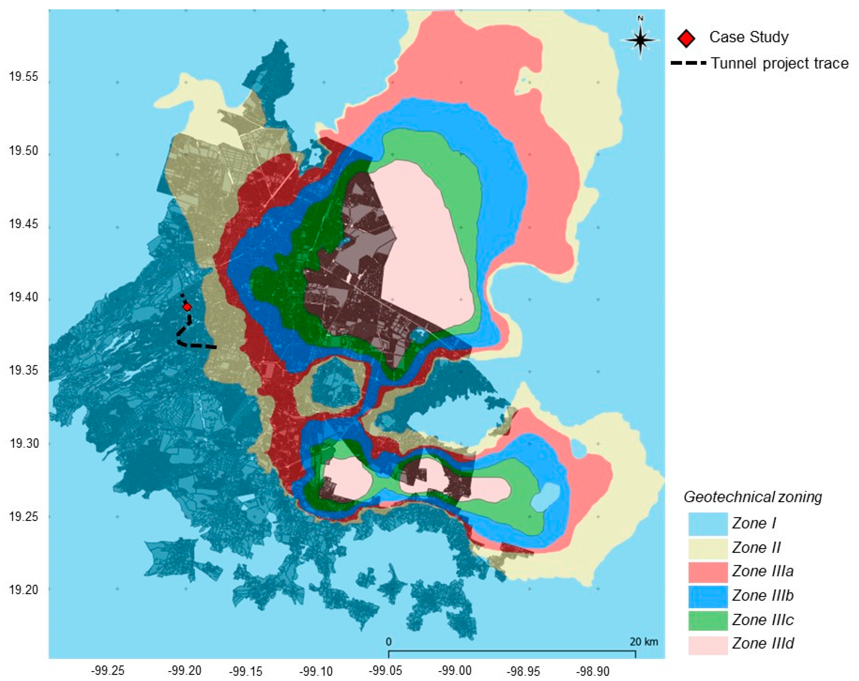
2. Case Study
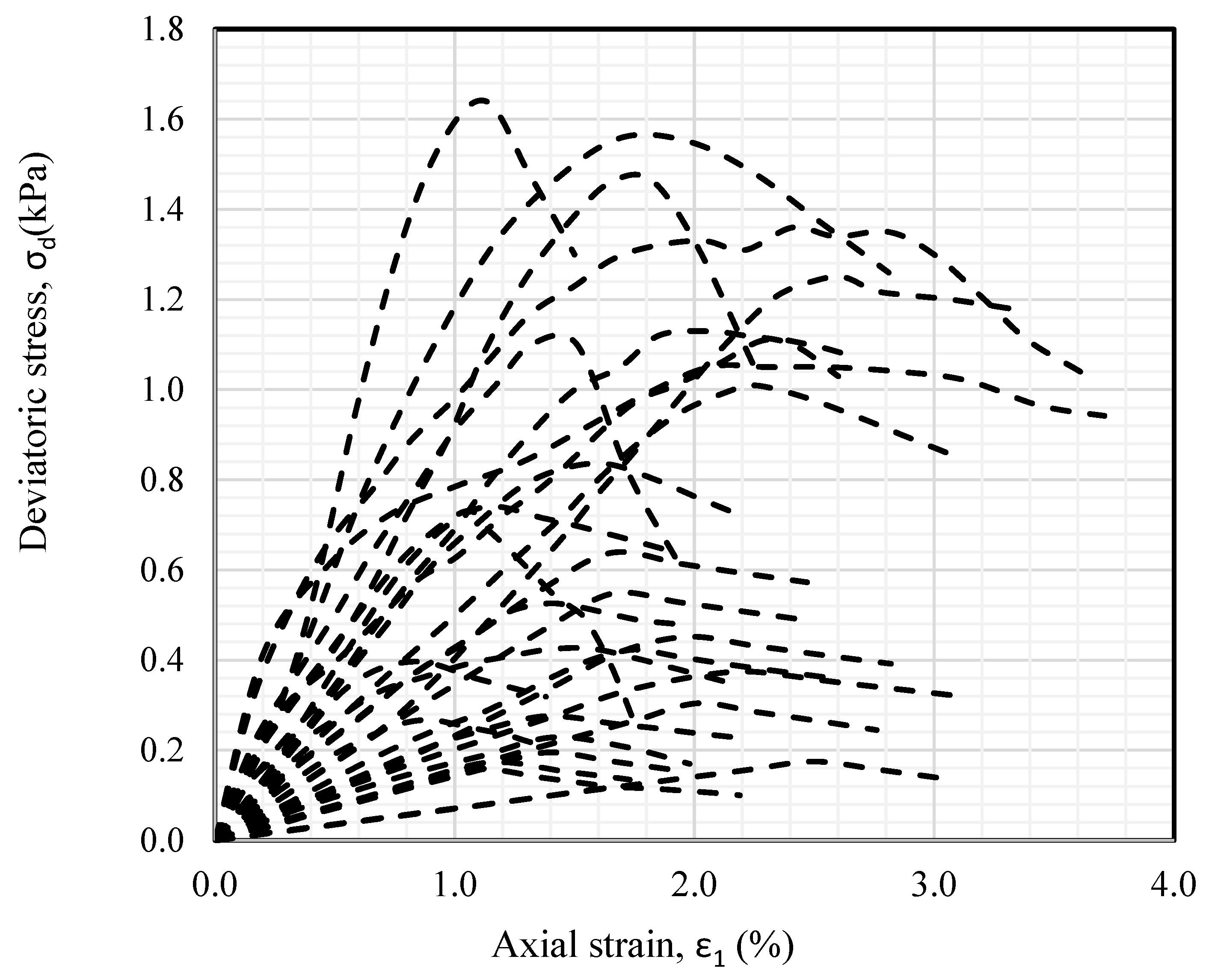
2.1. Geotechnical Conditions
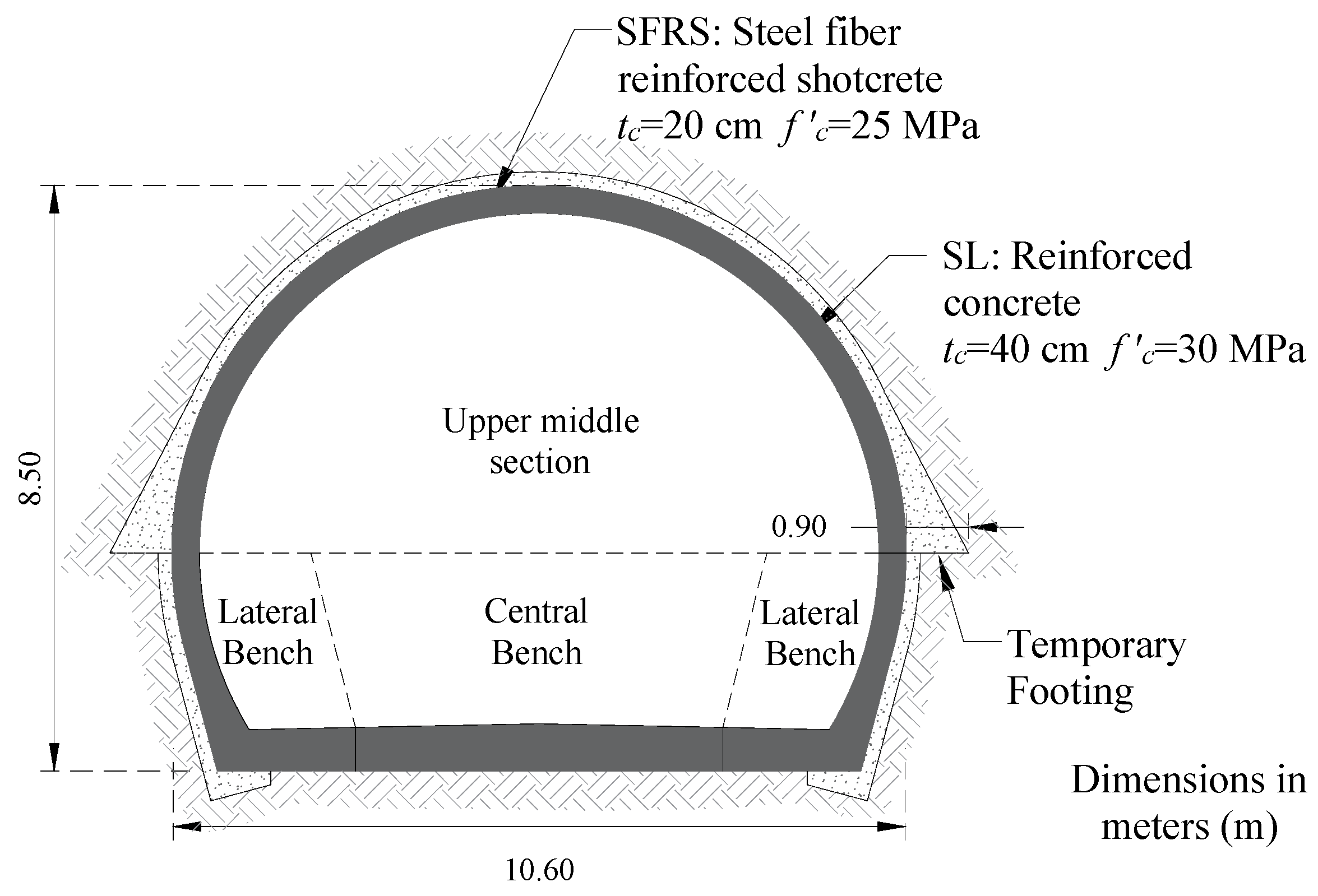
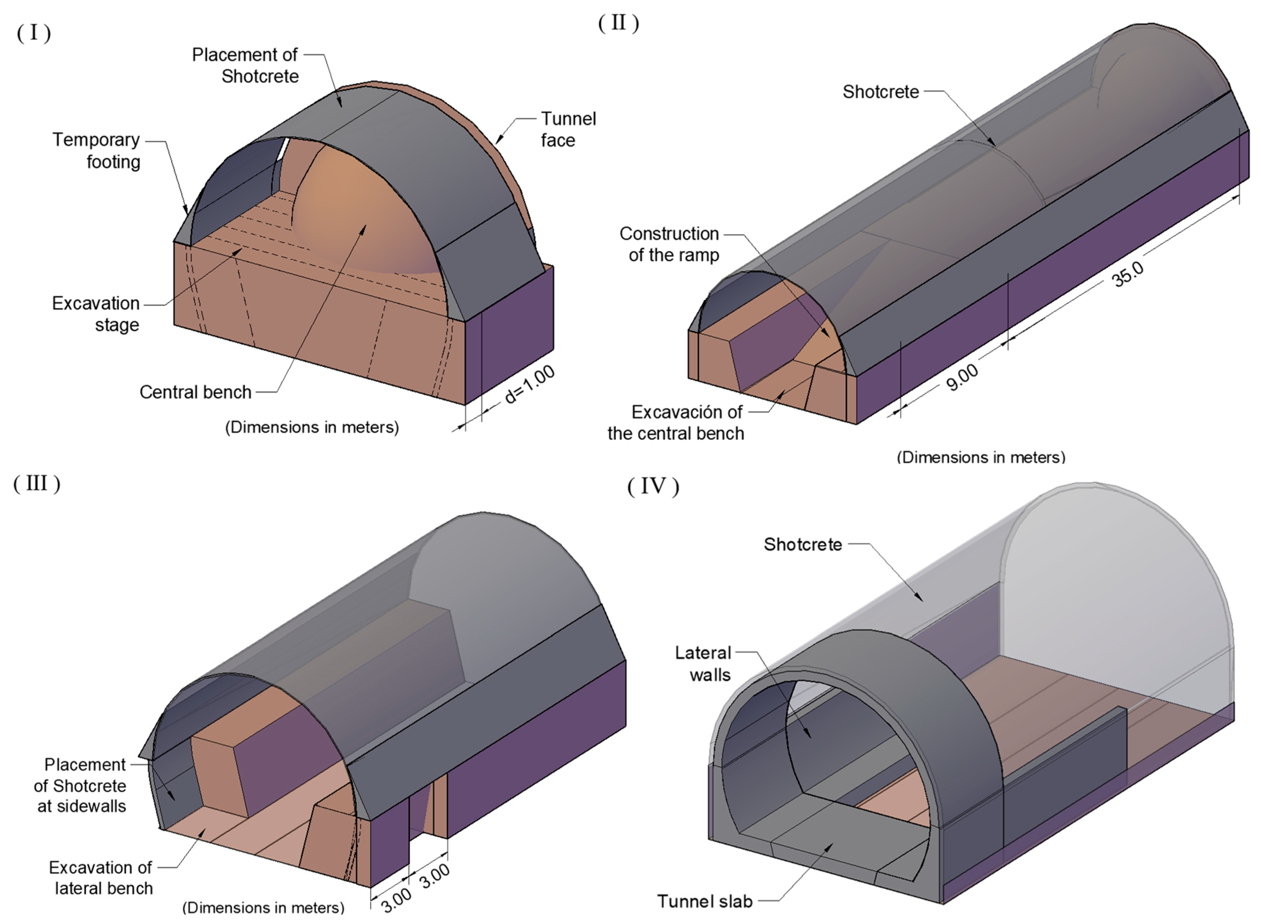
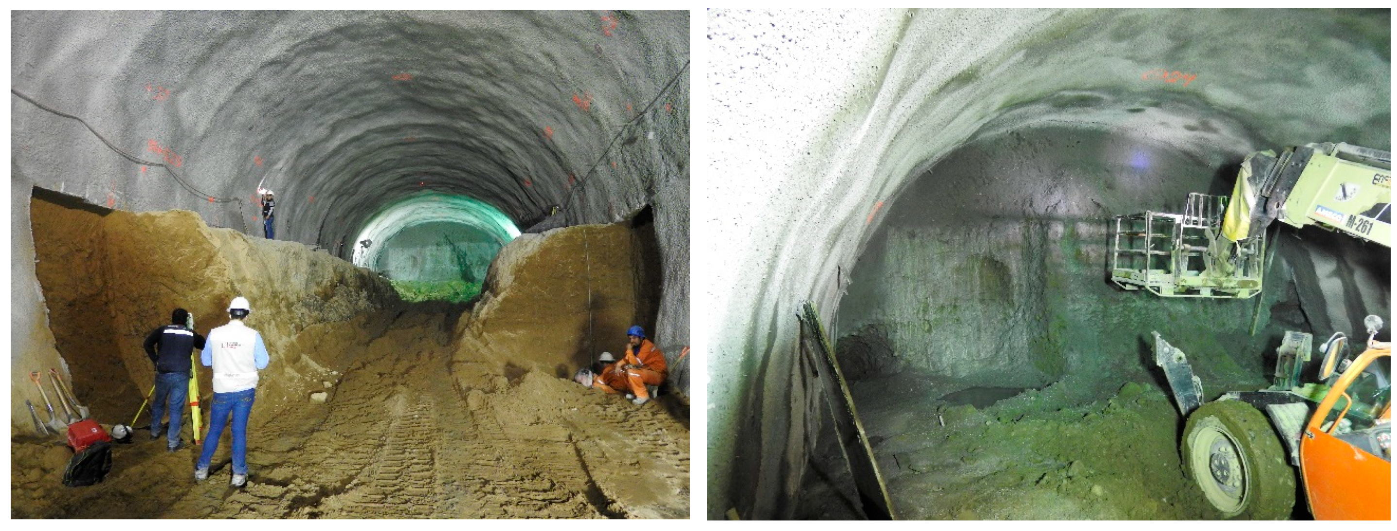
2.2. Tunnel Geometry and Excavation Process
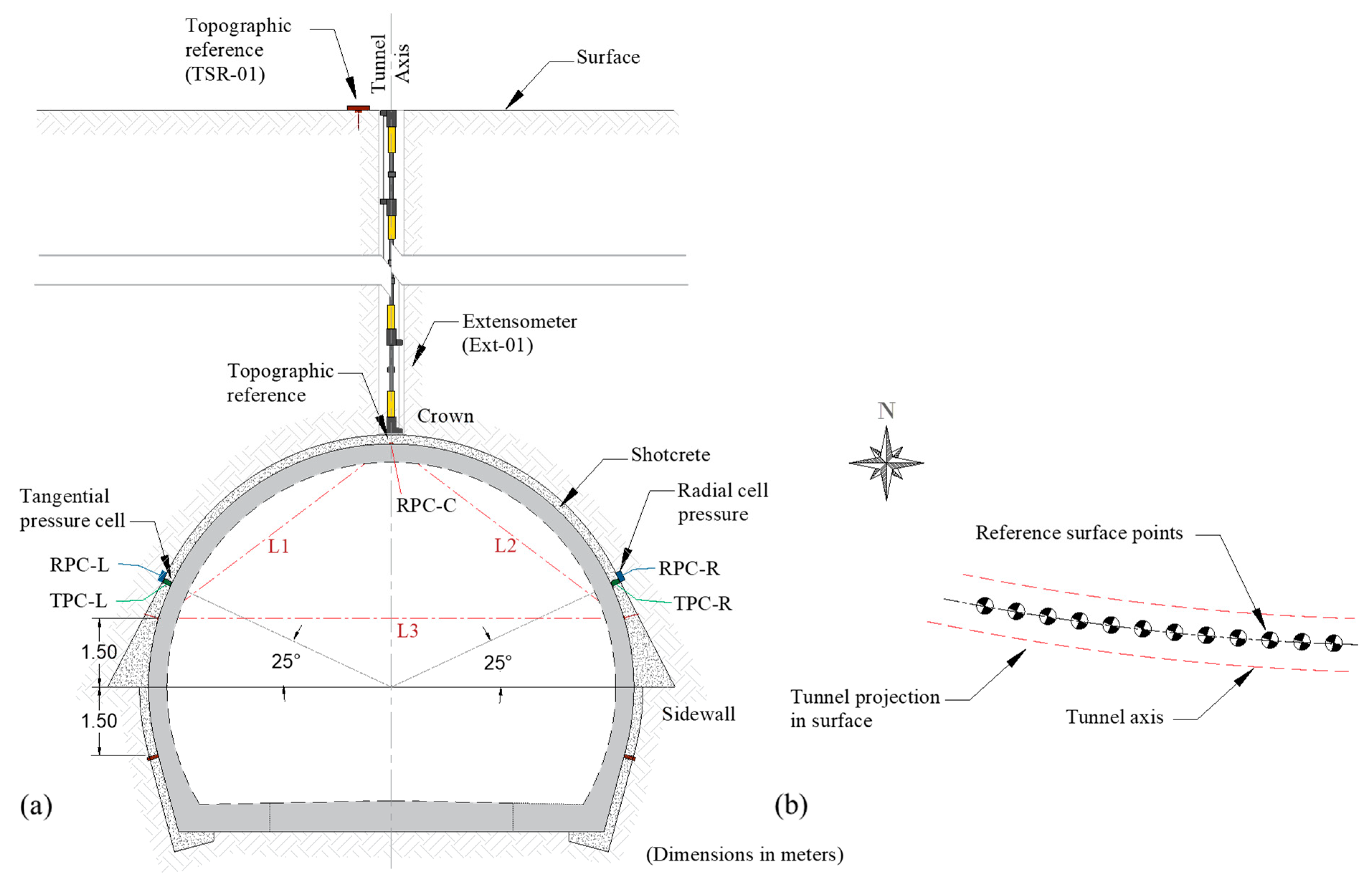
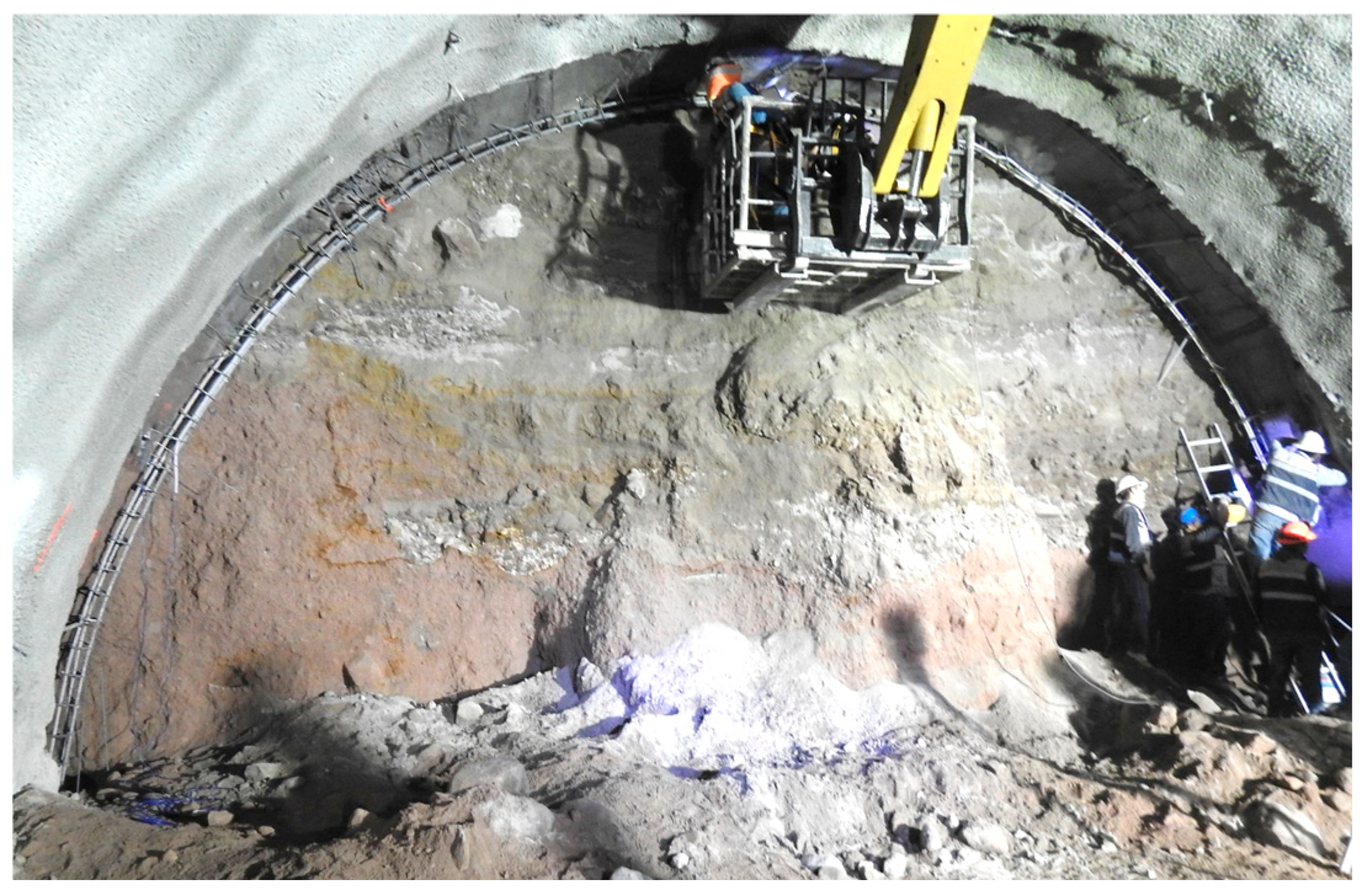
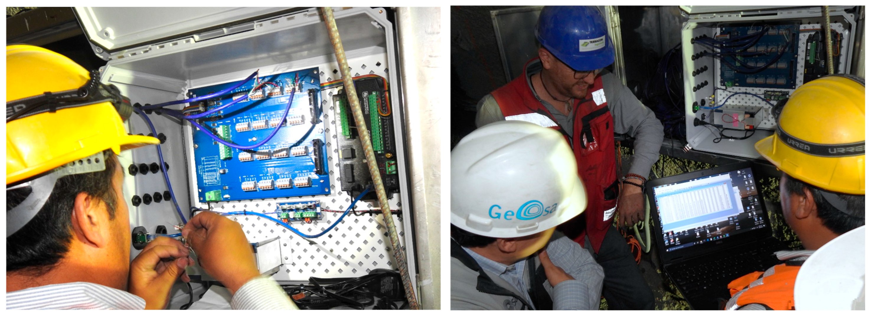
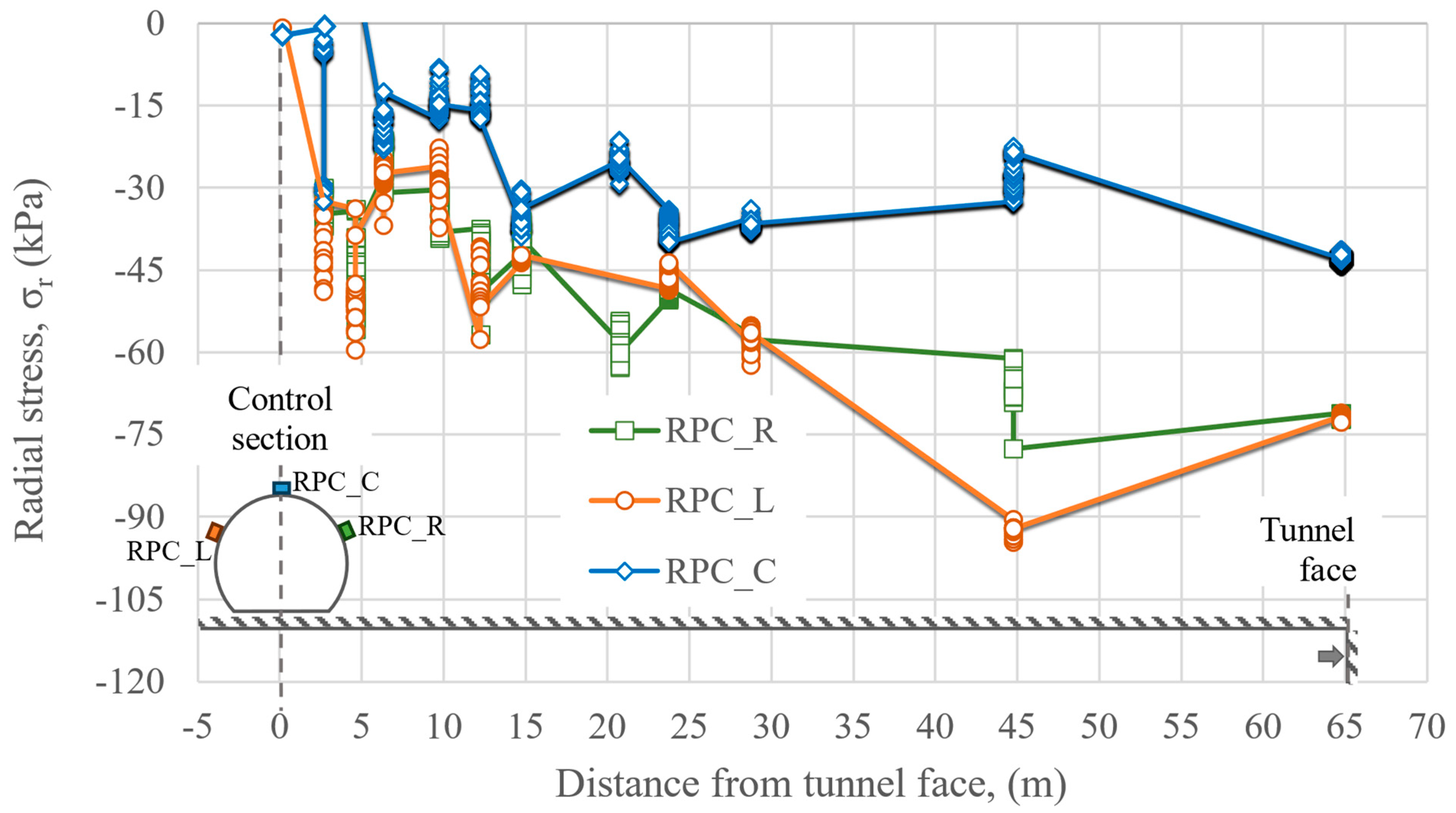
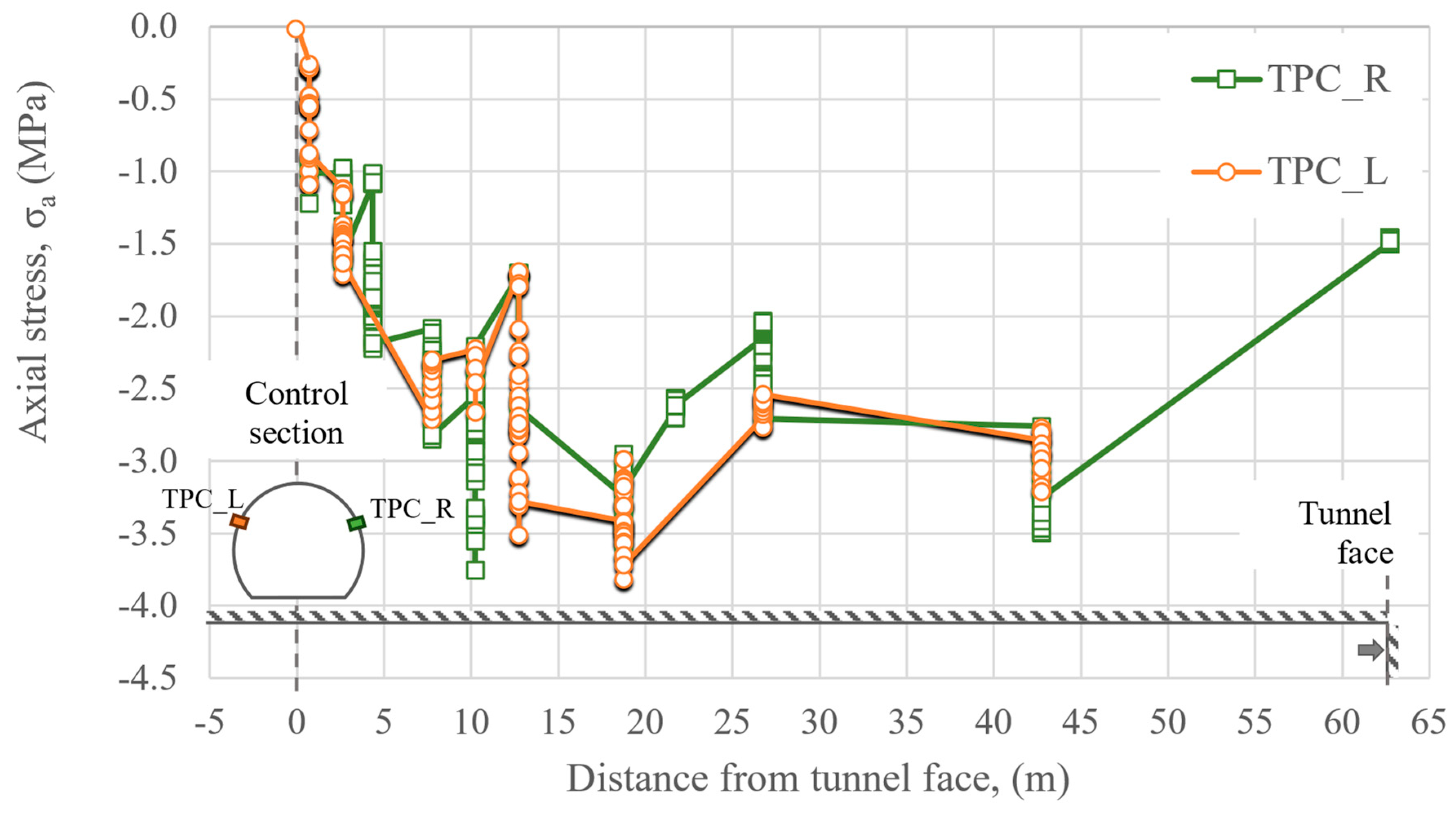
3. Tunnel Instrumentation
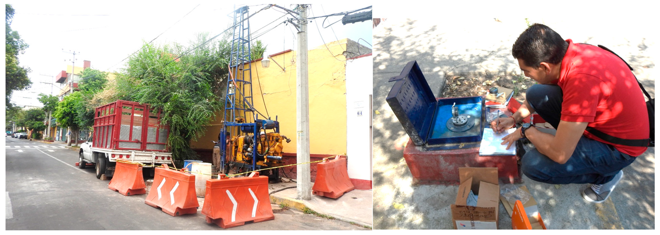
- Preparation of the installation area:
- 2.
- Marking of the location:
- 3.
- Drilling and hole preparation to fix the load cells to the soil:
- 4.
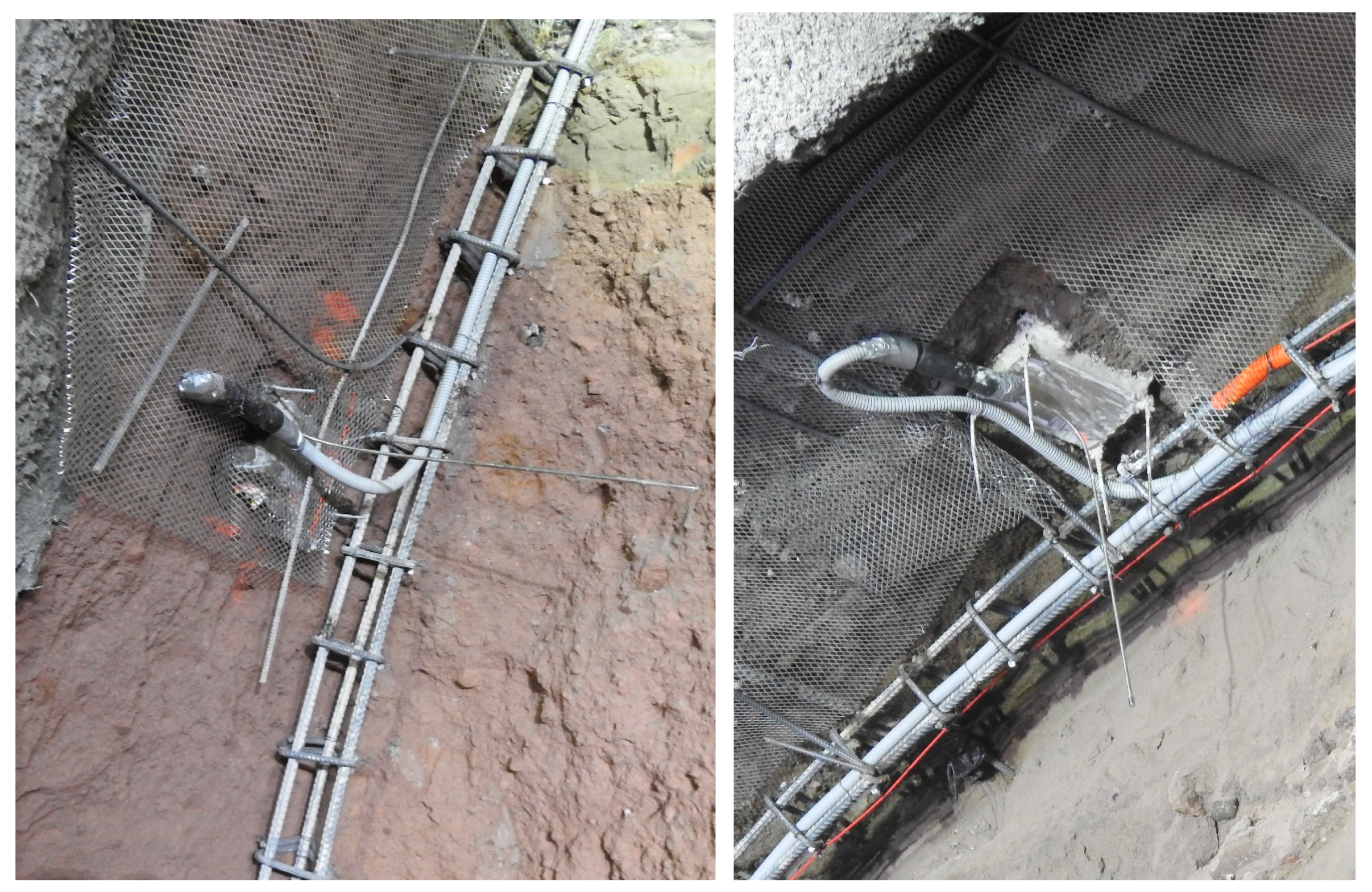
- Installation of the cells:
- 5.
- Instrumentation connection:
- 6.
- Testing and Calibration:
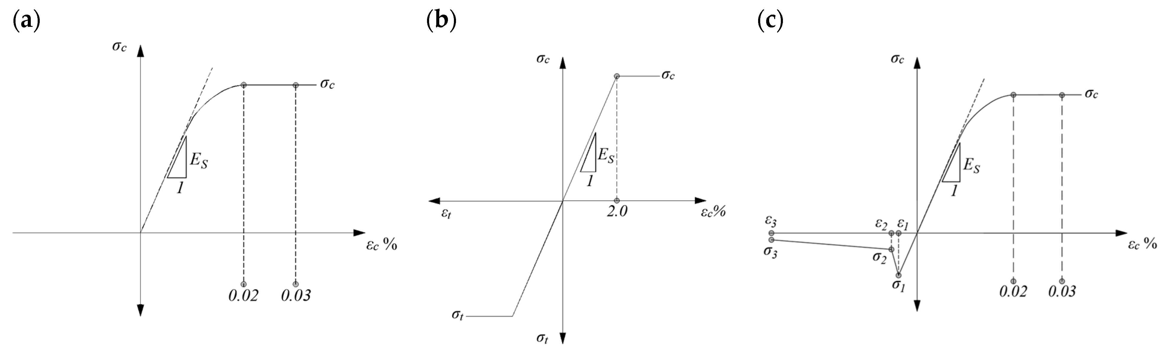
4. Numerical Modelling
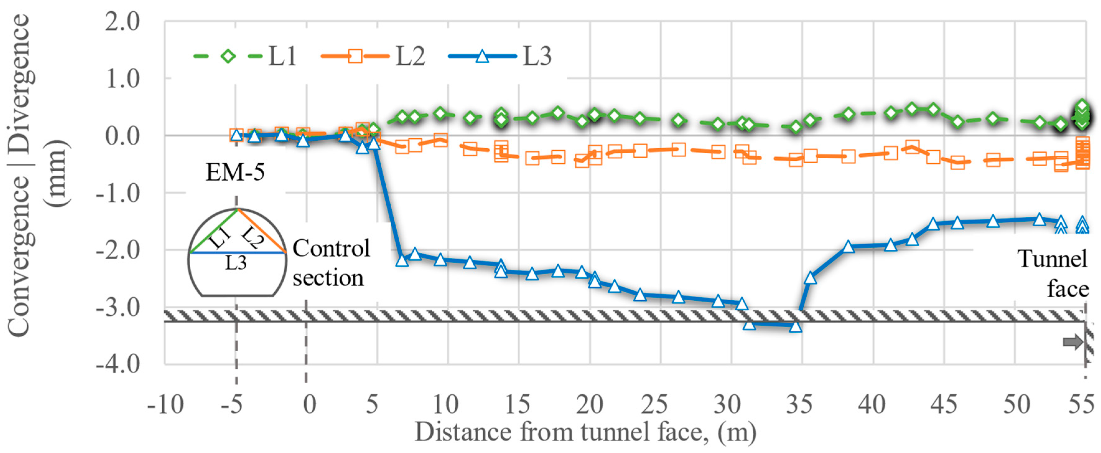
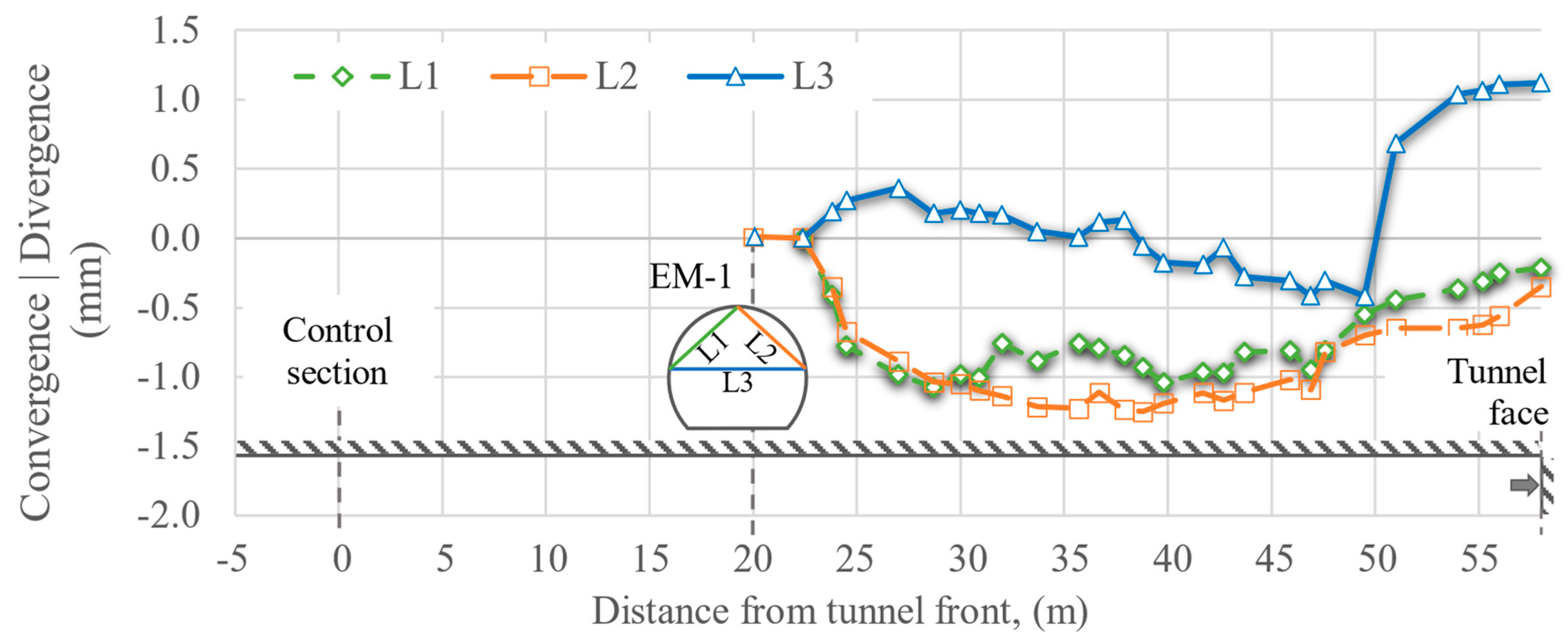
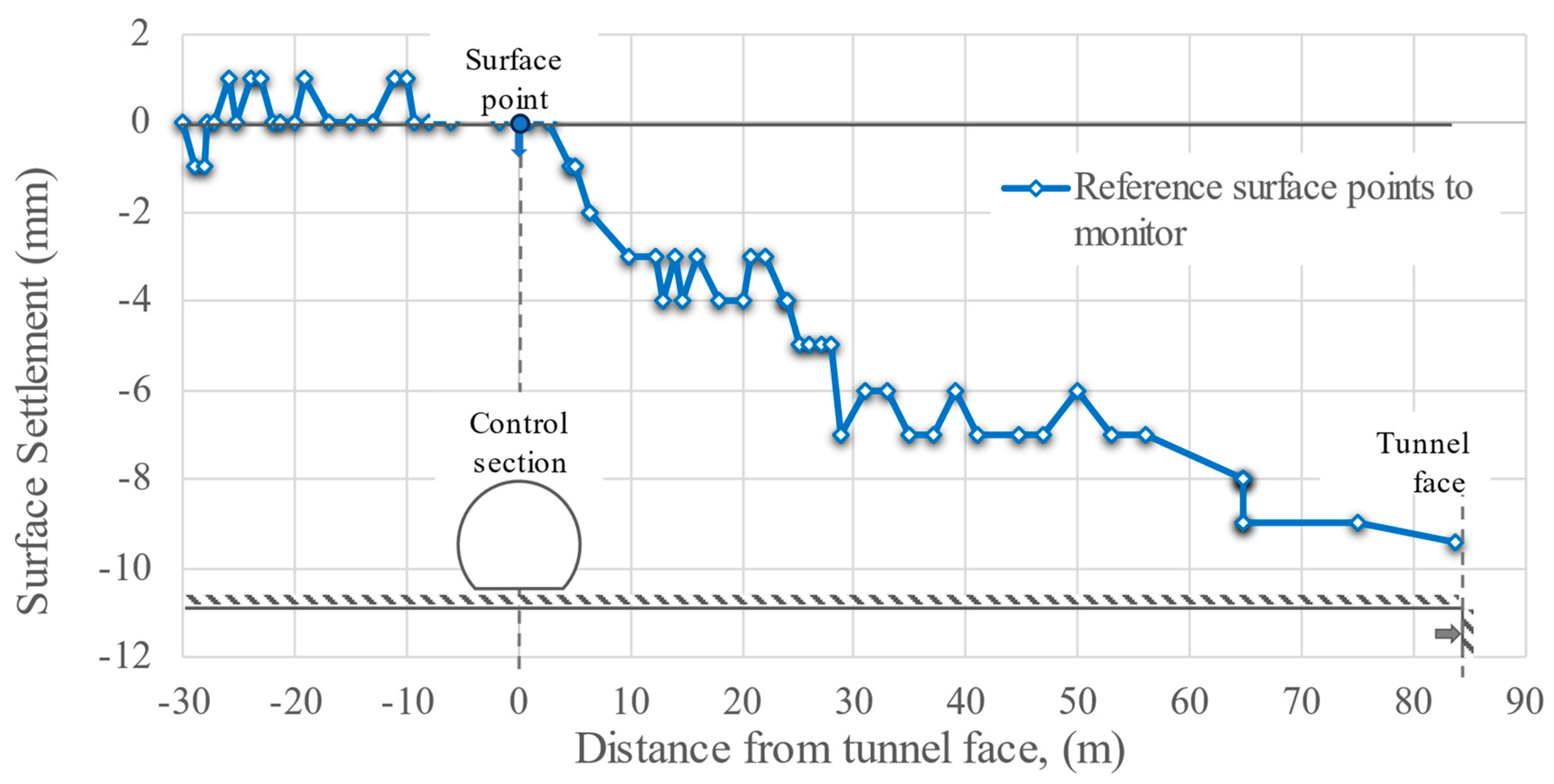
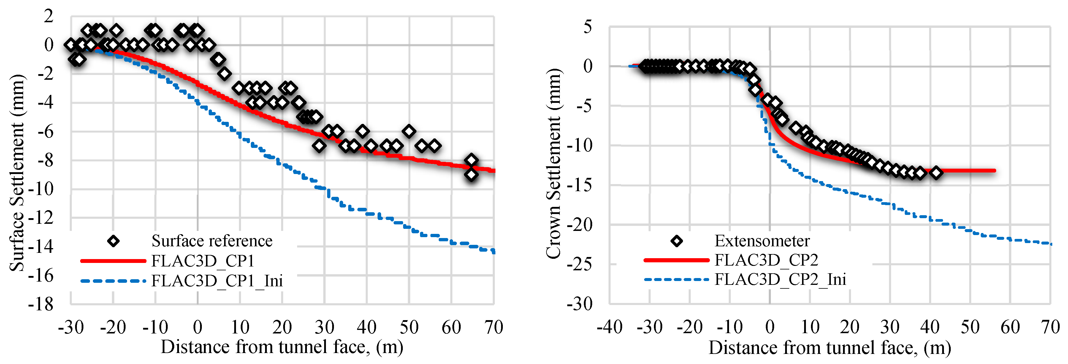
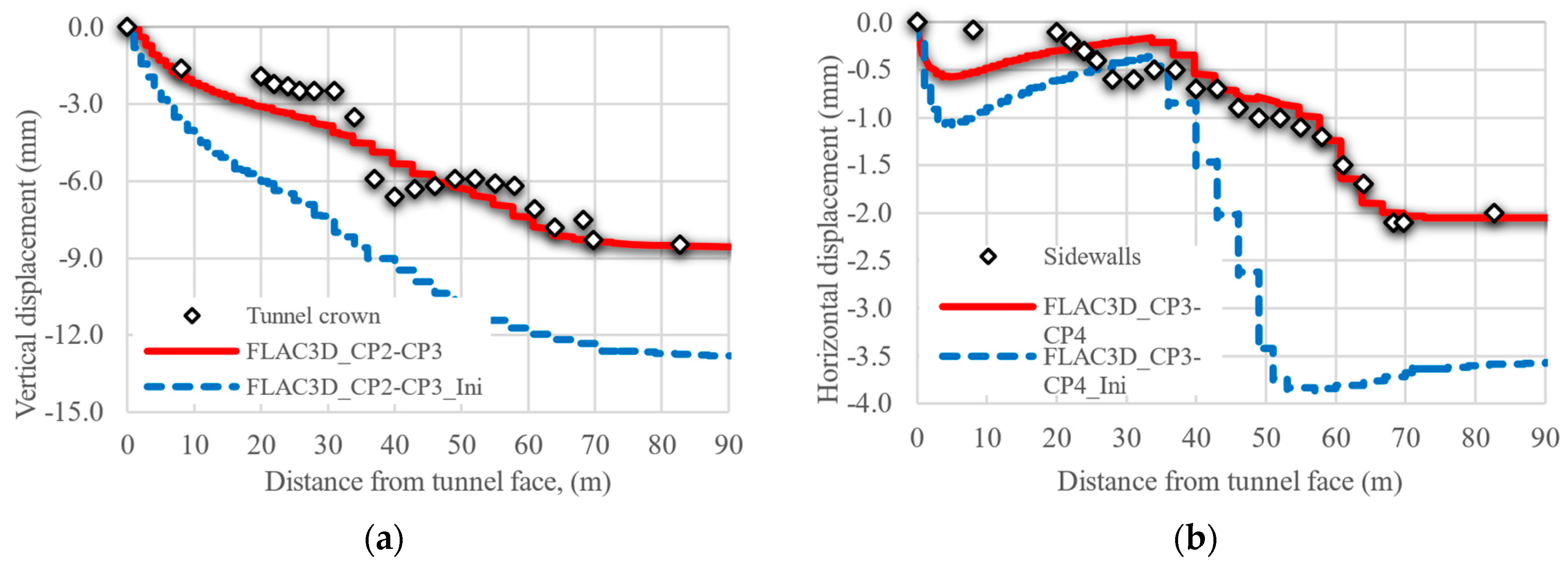
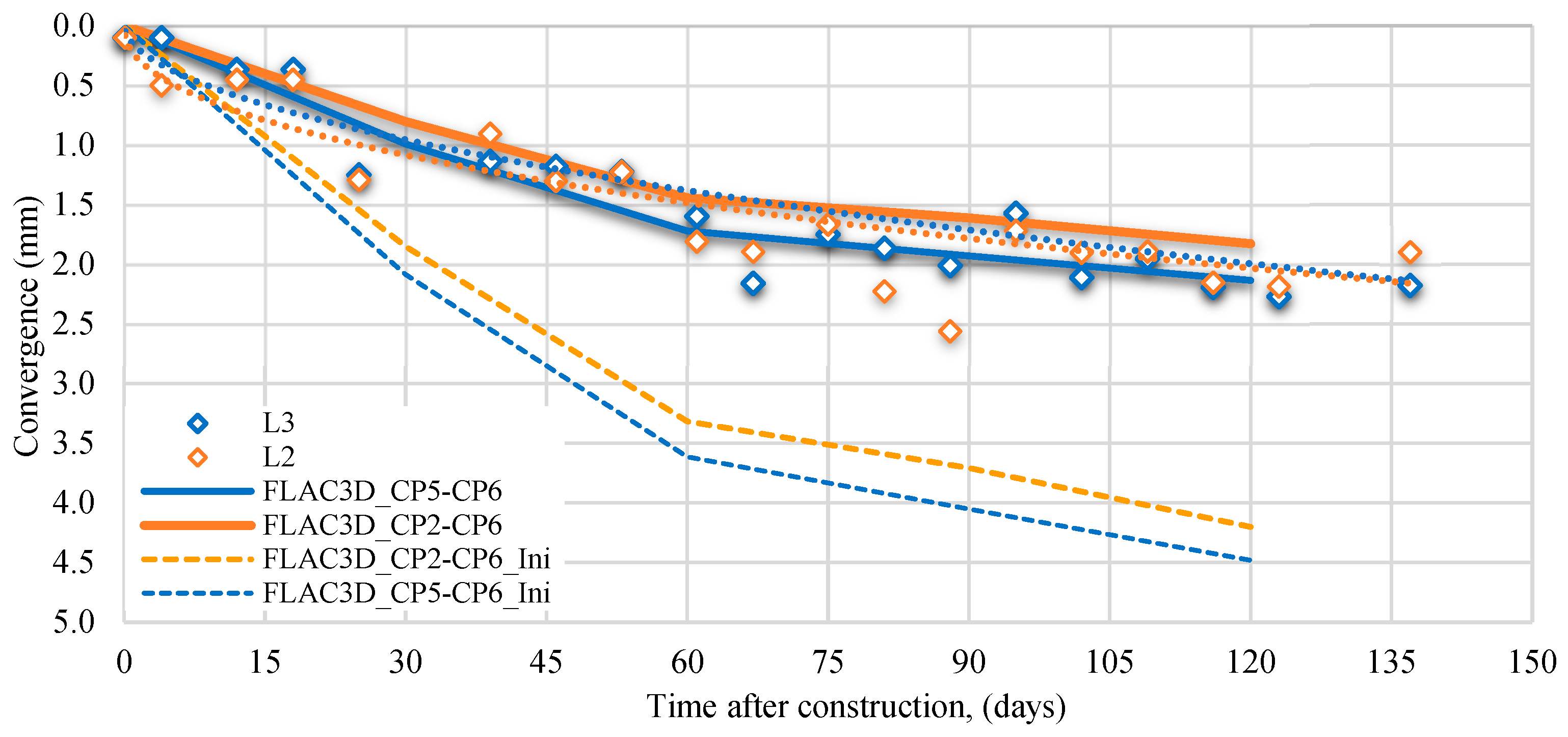
Model Prediction and Back-Analyses
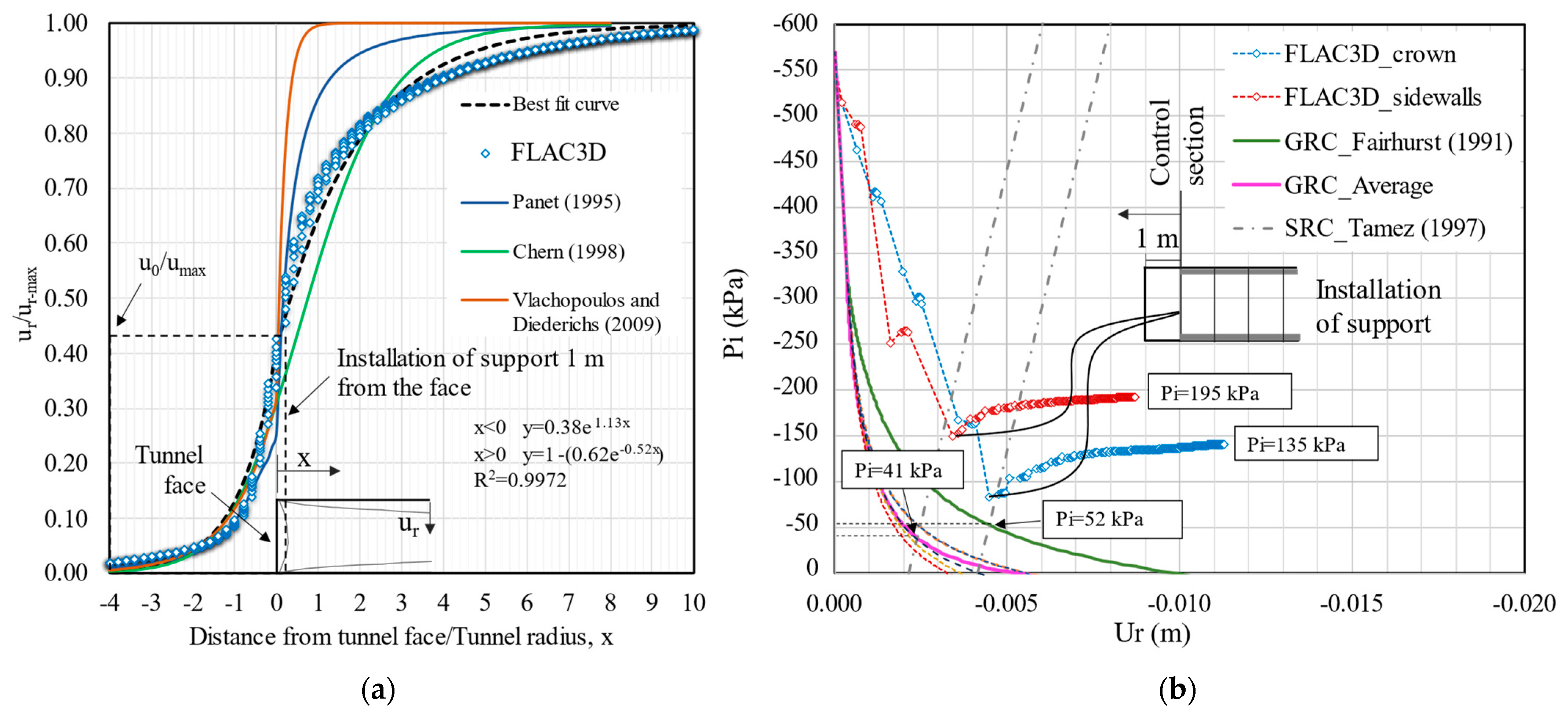
5. Comparison with Analytical Methods
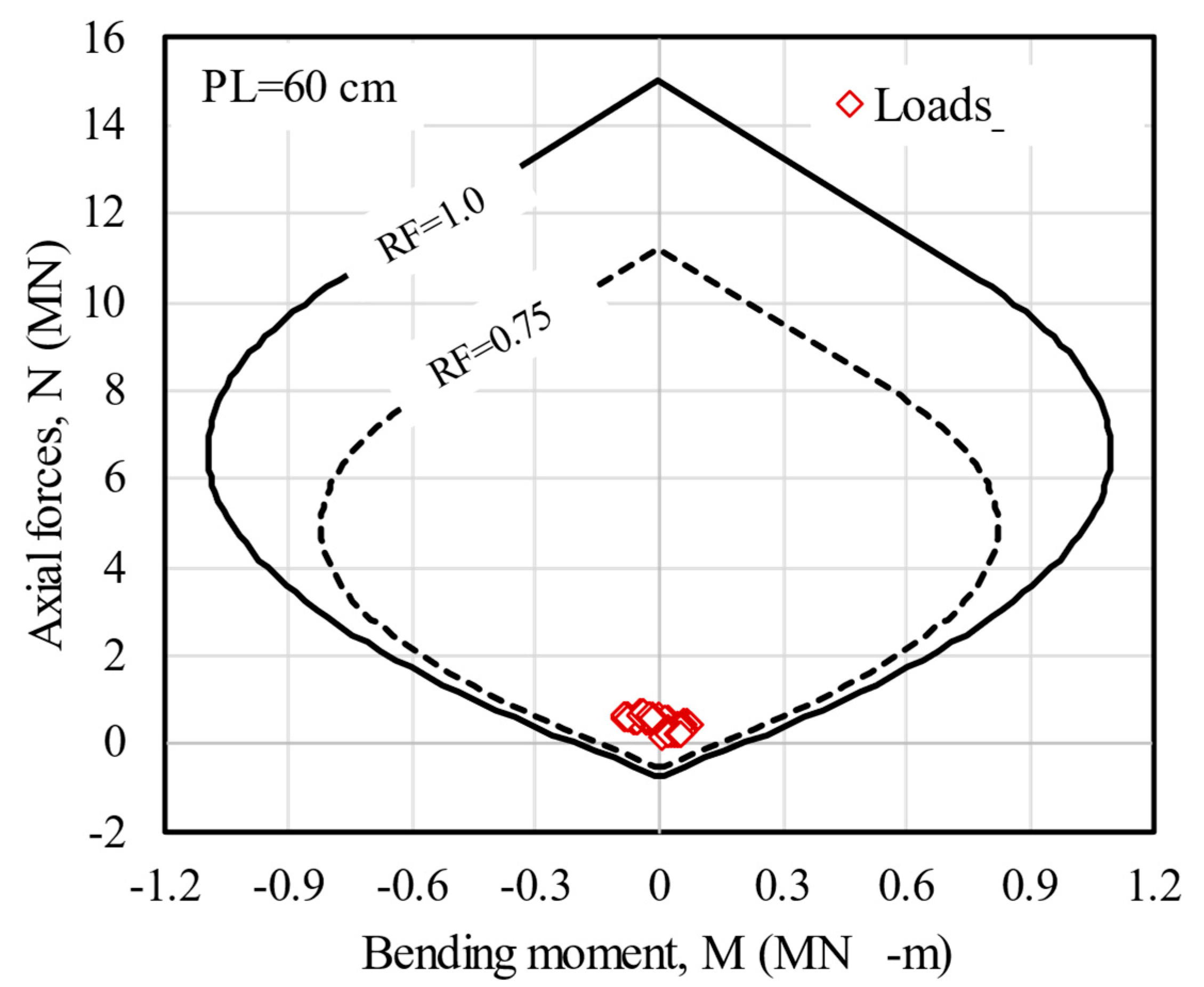
6. Optimization of Tunnel Lining Performance
7. Conclusions
- Instrumentation: The complexity during the installation of the instruments can affect the accuracy of the data obtained, as well as soil heterogeneities which lead to an irregular contact surface between the load cell and the adjacent soil.
- Single control section: Only one control section was instrumented. Ideally, two or three additional sections should have been installed to compare the results among several cases and observe the tunnel performance under different geotechnical conditions and tunnel coverages for a better generalization of the results.
- Surface loads: The consideration of loads due to traffic on the roadways, especially in the tunnel sections with low cover, can influence the final conclusions.
- External factors: Aspects such as climate conditions, groundwater, and seismic loading were not considered in this study.
Author Contributions
Funding
Institutional Review Board Statement
Informed Consent Statement
Data Availability Statement
Conflicts of Interest
References
- Mayoral, J.M. Performance evaluation of tunnels built in rigid soils. Tunn. Undergr. Space Technol. 2014, 43, 1–10. [Google Scholar] [CrossRef]
- Mayoral, J.M.; Melis-Maynar, M.J.I.; de la Sancha, A.R. Integral Approach of Performance-Based Design for Tunnels. Transp. Res. Rec. J. Transp. Res. Board 2015, 2522, 121–130. [Google Scholar] [CrossRef]
- de Ágreda, E.A.P. Failures Inspire Progress: Protecting Sensitive Buildings from Tunnelling. GeoStrata Mag. Arch. 2019, 23, 34–39. [Google Scholar] [CrossRef]
- Oliver, A. Heathrow trial runs under question. New Civil Engineer. 3 November 1994; 4–5. [Google Scholar]
- Oliver, A. Rush to stabilise Heathrow chasm. Int. J. Rock Mech. Min. Sci. Geomech. Abstr. 1995, 4, 189A. [Google Scholar]
- Sousa, R.L.; Einstein, H.H. Lessons from accidents during tunnel construction. Tunn. Undergr. Space Technol. 2021, 113, 103916. [Google Scholar] [CrossRef]
- Dong, Z.; Zhang, X.; Tong, C.; Chen, X.; Feng, H.; Zhang, S. Grouting-induced ground heave and building damage in tunnel construction: A case study of Shenzhen metro. Undergr. Space 2022, 7, 1175–1191. [Google Scholar] [CrossRef]
- Lim, C.X.; Jusoh, S.N.; Lim, C.B.; Abdullah, R.A.; Yunus, N.Z.M. Tunnel depth effect to pile in Tunnel’s influence zone. Phys. Chem. Earth 2023, 129, 103298. [Google Scholar] [CrossRef]
- Son, M. Response analysis of nearby structures to tunneling-induced ground movements in sandy soils. Tunn. Undergr. Space Technol. 2015, 48, 156–169. [Google Scholar] [CrossRef]
- Son, M. Response analysis of nearby structures to tunneling-induced ground movements in clay soils. Tunn. Undergr. Space Technol. 2016, 56, 90–104. [Google Scholar] [CrossRef]
- ITA. General Report on Conventional Tunnelling Method; International Tunnelling and Underground Space Association: Chatelaine-Geneve, Switzerland, 2009; p. 27. [Google Scholar]
- Behnen, G.; Nevrly, T.; Fischer, O. Soil-structure interaction in tunnel lining analyses. Geotechnik 2015, 38, 96–106. [Google Scholar] [CrossRef]
- Bierbaumer, A.H. Die Dimensionierung Des Tunnel Manerwerks; W. Engelmann: Liepzig, Germany, 1913. [Google Scholar]
- Szechy, K. The Art of Tunnelling; Akademiai Kaido: Budapest, Hungary, 1970. [Google Scholar]
- Terzaghi, K. Introduction to Tunnel Geology in Rock Tunneling Withsteel Supports; The Commercial Shearing and Stamping Co.: Youngstown, OH, USA, 1964. [Google Scholar]
- Bin, L.; Liu, X.; Xu, M. Reliability Analysis of Primary Supports in Deep and Soft-rock Tunnel Based on Probabilistic Design Numerical Method. Electron. J. Geotech. Eng. 2016, 21, 5013–5028. [Google Scholar]
- Einstein, H.H.; Schwartz, C.W. Simplified Analysis for Tunnel Support. J. Geotech. Eng. Div. 1979, 105, 499–518. [Google Scholar] [CrossRef]
- Ghorbani, A.; Hasanzadehshooiili, H. A comprehensive solution for the calculation of ground reaction curve in the crown and sidewalls of circular tunnels in the elastic-plastic-EDZ rock mass considering strain softening. Tunn. Undergr. Space Technol. 2019, 84, 413–431. [Google Scholar] [CrossRef]
- Oreste, P. The convergence-confinement method: Roles and limits in modern geomechanical tunnel design. Am. J. Appl. Sci. 2009, 6, 757–771. [Google Scholar] [CrossRef]
- Panet, M.; Bouvard, A.; Dardard, B.; Dubois, P.; Givet, O.; Guilloux, A.; Launay, J.; Duc, N.M.; Piraud, J.; Tournery, H.; et al. The Convergence-Confinement Method AFTES–Recommendations des Groupes Travait; French Association of Tunnels and Underground Space (AFTES): Paris, France, 2001. [Google Scholar]
- Oreste, P.P. A Procedure for Determining the Reaction Curve of Shotcrete Lining Considering Transient Conditions. Rock Mech. Rock Eng. 2003, 36, 209–236. [Google Scholar] [CrossRef]
- Verman, M.; Singh, B.; Jethwa, J.L.; Viladkar, M.N. Determination of Support Reaction Curve for Steel-Supported Tunnels. Tunn. Undergr. Space Technol. 1995, 10, 217–224. [Google Scholar] [CrossRef]
- Wang, Y.Q.; Luo, M.R. Analysis of Support Reaction Curves considering Time-Varying Effect of Shotcrete. Adv. Civ. Eng. 2020, 2020, 6069432. [Google Scholar] [CrossRef]
- Sadeghiyan, R.; Hashemi, M.; Moloudi, E. Determination of longitudinal convergence profile considering effect of soil strength parameters. Int. J. Rock Mech. Min. Sci. 2016, 82, 10–21. [Google Scholar] [CrossRef]
- Vlachopoulos, N.; Diederichs, M.S. Improved Longitudinal Displacement Profiles for Convergence Confinement Analysis of Deep Tunnels. Rock Mech. Rock Eng. 2009, 42, 131–146. [Google Scholar] [CrossRef]
- Argyroudis, S.; Tsinidis, G.; Gatti, F.; Pitilakis, K. Effects of SSI and lining corrosion on the seismic vulnerability of shallow circular tunnels. Soil Dyn. Earthq. Eng. 2017, 98, 244–256. [Google Scholar] [CrossRef]
- Guo, X.; Du, D.; Dias, D. Reliability analysis of tunnel lining considering soil spatial variability. Eng. Struct. 2019, 196, 11. [Google Scholar] [CrossRef]
- Hamrouni, A.; Dias, D.; Sbartai, B. Reliability analysis of shallow tunnels using the response surface methodology. Undergr. Sp. 2017, 2, 246–258. [Google Scholar] [CrossRef]
- Mayoral, J.M.; Mosqueda, G.; De La Rosa, D.; Alcaraz, M. Tunnel performance during the Puebla-Mexico 19 September 2017 earthquake. Earthq. Spectra 2020, 36, 288–313. [Google Scholar] [CrossRef]
- Mayoral, J.M.; Mosqueda, G. Foundation enhancement for reducing tunnel-building seismic interaction on soft clay. Tunn. Undergr. Space Technol. 2021, 115, 104016. [Google Scholar] [CrossRef]
- Panet, M.; Guenot, A. Analysis of convergence behind the face of a tunnel: Tunnelling 82. In Proceedings of the 3rd International Symposium, Brighton, UK, 7–11 June 1982; International Journal of Rock Mechanics and Mining Sciences & Geomechanics Abstracts; IMM: London, UK, 1982; Volume 20, pp. 197–204. [Google Scholar]
- Pitilakis, K.; Tsinidis, G.; Leanza, A.; Maugeri, M. Seismic behaviour of circular tunnels accounting for above ground structures interaction effects. Soil Dyn. Earthq. Eng. 2014, 67, 1–15. [Google Scholar] [CrossRef]
- Wood, D.M. Geotechnical Modelling; Taylor y Francis; CRC Press: Boca Raton, FL, USA, 2004. [Google Scholar]
- He, B.M.; Zhang, X.W.; Li, H.P. Ground load on tunnels built using new Austrian tunneling method: Study of a tunnel passing through highly weathered sandstone. Bull. Eng. Geol. Environ. 2019, 78, 6221–6234. [Google Scholar] [CrossRef]
- Karakus, M.; Fowell, R.J. Back analysis for tunnelling induced ground movements and stress redistribution. Tunn. Undergr. Space Technol. 2005, 20, 514–524. [Google Scholar] [CrossRef]
- Zhang, D.; Fang, Q.; Li, P.; Wong, L.N.Y. Structural Responses of Secondary Lining of High-Speed Railway Tunnel Excavated in Loess Ground. Adv. Struct. Eng. 2013, 16, 1371–1379. [Google Scholar] [CrossRef]
- Ng, C.W.W.; Lu, H.; Peng, S.Y. Three-dimensional centrifuge modelling of the effects of twin tunnelling on an existing pile. Tunn. Undergr. Space Technol. 2013, 35, 189–199. [Google Scholar] [CrossRef]
- Nomoto, T.; Imamur, S.; Hagiwara, T.; Kusakabe, O.; Fujii, N. Shield Tunnel Construction in Centrifuge. J. Geotech. Geoenvironmental Eng. 1999, 125, 237–345. [Google Scholar] [CrossRef]
- Song, G.; Arshall, A.M. Centrifuge modelling of tunnelling induced ground displacements: Pressure and displacement control tunnels. Tunn. Undergr. Space Technol. 2020, 103, 103461. [Google Scholar] [CrossRef]
- Mayoral, J.M.; Alcaraz, M.; Tepalcapa, S. Seismic performance of soil–tunnel–building systems in stiff soils. Earthq. Spectra 2023, 39, 1214–1239. [Google Scholar] [CrossRef]
- Hettiarachchi, H.; Brown, T. Use of SPT Blow Counts to Estimate Shear Strength Properties of Soils: Energy Balance Approach. J. Goetechnical Geoenviromental Eng. 2009, 135, 830–834. [Google Scholar] [CrossRef]
- American Association of State Highway and Transportation Officials (AASHTO). LRFD Bridge Design Specifications; AASHTO: Washington, DC, USA, 2012. [Google Scholar]
- Itasca Consulting Group. FLAC, Fast Lagragian Analysis of Continua. User’s Guide; Itasca Consulting Group, Inc.: Minneapolis, MN, USA, 2009. [Google Scholar]
- Panet, M. Calcul des Tunnels par la Me’thode de Convergence—Confinement; Presses del’Ecole Nationale des Ponts et Chausse’es: Paris, France, 1995; p. 178. [Google Scholar]
- Alonso, E.; Alejano, L.R.; Varas, F.; Fdez-Manin, G.; Carranza-Torres, C. Ground response curves for rock masses exhibiting strain-softening behavior. Int. J. Numer. Anal. Methods Geomech. 2003, 27, 1153–1185. [Google Scholar] [CrossRef]
- Stille, H.; Holmberg, M.; Nord, G. Support of weak rock with grouted bolts and shtocrete. Internatinal J. Rock Mech. Min. Sci. 1989, 26, 99–113. [Google Scholar] [CrossRef]
- Tamez, E.; Rangel, J.L.; Y Holguin, E. Diseño Geotécnico de Túneles; TGC Geotecnia: Mexico City, Mexico, 1997. (In Spanish) [Google Scholar]
- Fairhurst, C. General philosophy of support design for underground structures in hard rock. Undergr. Struct. Des. Constr. 1991, 59, 1–55. [Google Scholar]
- Chern, J.C.; Shiao, F.Y.; Yu, C.W. An Empirical Safety Criterion for Tunnel Construction: Proceedings of the Regional Symposium on Sedimentary Rock Engineering; Public Construction Commission: Taipei, Taiwan, 1998; pp. 222–227. [Google Scholar]
- Kaiser, P. Rational assessment of tunnel liner capacity. In Proceedings of the 5th Canadian Tunneling Conference, Montreal, QC, Canada; 1985. [Google Scholar]
- Sauer, G.; Gall, V.; Bauer, E.; Dietmaier, P. Design of tunnel concrete linings using limit capacity curves. In Proceedings of the 8th International Conference on Computer Methods and Advances in Geomechanics, Morgantown, WV, USA, 22–28 May 1994; pp. 2621–2626. [Google Scholar]
- Vandewalle, L. Recommendations of RILEM TC 162-TDF: Test and design methods for steel fibre reinforced concrete. Mater. Struct. Mater. Constr. 2000, 33, 3–5. [Google Scholar]


| Layer | USCS | NSPT (Blows Counts) | γ (kN/m3) | c (kPa) | φ (°) | E50 (MPa) | ν (-) |
|---|---|---|---|---|---|---|---|
| UG-1 | ML | 42 | 15.8 | 18 | 28 | 120.8 | 0.32 |
| UG-2 | SM | 167 | 18.2 | 45 | 29 | 900.4 | 0.28 |
| UG-3 | CL-ML | 40 | 17 | 13 | 27 | 97.5 | 0.34 |
| UG-4 | ML | 126 | 18.2 | 40 | 28 | 470.5 | 0.28 |
| UG-5 | SC | 80 | 19.2 | 33 | 31 | 303.2 | 0.27 |
| Sensor ID | Instrumentation | Variables Measured |
|---|---|---|
| L1, L2 and L3 | Convergences and divergences | Tunnel distortion |
| TSR-01 | Reference surface points | Surface settlements |
| Ext-01 | Extensometer | Tunnel crown settlements |
| RPC-L, RPC-R and RPC-C | Radial pressure cells | Radial stress on primary lining |
| TPC-L and TPC-R | Tangential pressure cells | Axial stress on primary lining |
| Layer | USCS | NSPT (Blows Counts) | γ (kN/m3) | c (kPa) | φ (°) | E50 (MPa) | ν (-) |
|---|---|---|---|---|---|---|---|
| UG-1 | ML | 51 | 15.8 | 20.5 | 28 | 160 | 0.32 |
| UG-2 | SM | 167 | 18.2 | 51.2 | 30 | 970 | 0.28 |
| UG-3 | CL-ML | 40 | 17 | 15.6 | 27 | 123 | 0.34 |
| UG-4 | ML | 126 | 18.2 | 47.5 | 28 | 590 | 0.28 |
| UG-5 | SC | 80 | 19.2 | 36.3 | 32 | 445 | 0.27 |
| Case | Primary Lining Thickness (m) | Secondary Lining Thickness (m) |
|---|---|---|
| 1 | 0.2 | 0.4 |
| 2 | 0.3 | 0.3 |
| 3 | 0.4 | 0.2 |
| 4 | 0.6 | --- |
Disclaimer/Publisher’s Note: The statements, opinions and data contained in all publications are solely those of the individual author(s) and contributor(s) and not of MDPI and/or the editor(s). MDPI and/or the editor(s) disclaim responsibility for any injury to people or property resulting from any ideas, methods, instructions or products referred to in the content. |
© 2024 by the authors. Licensee MDPI, Basel, Switzerland. This article is an open access article distributed under the terms and conditions of the Creative Commons Attribution (CC BY) license (https://creativecommons.org/licenses/by/4.0/).
Share and Cite
Suárez-Fino, J.F.; Mayoral, J.M. Numerical Modeling for Tunnel Lining Optimization. Appl. Sci. 2024, 14, 7415. https://doi.org/10.3390/app14167415
Suárez-Fino JF, Mayoral JM. Numerical Modeling for Tunnel Lining Optimization. Applied Sciences. 2024; 14(16):7415. https://doi.org/10.3390/app14167415
Chicago/Turabian StyleSuárez-Fino, Jose Francisco, and Juan M. Mayoral. 2024. "Numerical Modeling for Tunnel Lining Optimization" Applied Sciences 14, no. 16: 7415. https://doi.org/10.3390/app14167415
APA StyleSuárez-Fino, J. F., & Mayoral, J. M. (2024). Numerical Modeling for Tunnel Lining Optimization. Applied Sciences, 14(16), 7415. https://doi.org/10.3390/app14167415