Article

Visual Odometry in GPS-Denied Zones for Fixed-Wing Unmanned Aerial Vehicle with Reduced Accumulative Error Based on Satellite Imagery

by
Pablo Mateos-Ramirez
,
Javier Gomez-Avila
,
Carlos Villaseñor
and
Nancy Arana-Daniel
*
University Center for Exact Sciences and Engineering, University of Guadalajara, 1421 Marcelino García Barragán, Guadalajara 44430, Mexico
*
Author to whom correspondence should be addressed.
These authors contributed equally to this work.
Appl. Sci. 2024, 14(16), 7420; https://doi.org/10.3390/app14167420 (registering DOI)
Submission received: 11 July 2024 / Revised: 14 August 2024 / Accepted: 19 August 2024 / Published: 22 August 2024
(This article belongs to the Special Issue Advances in Unmanned Aerial Vehicle (UAV) System)

Abstract

:
In this paper, we present a method for estimating GPS coordinates from visual information captured by a monocular camera mounted on a fixed-wing tactical Unmanned Aerial Vehicle at high altitudes (up to 3000 m) in GPS-denied zones. The main challenge in visual odometry using aerial images is the computation of the scale due to irregularities in the elevation of the terrain. That is, it is not possible to accurately convert from pixels in the image to meters in space, and the error accumulates. The contribution of this work is a reduction in the accumulated error by comparing the images from the camera with satellite images without requiring the dynamic model of the vehicle. The algorithm has been tested in real-world flight experiments at altitudes above 1000 m and in missions over 17 km. It has been proven that the algorithm prevents an increase in the accumulated error.

1. Introduction

GPS (Global Positioning System) is crucial for Unmanned Aerial Vehicles (UAVs) because it provides accurate positioning and navigation, essential for various applications such as surveying, mapping, and search and rescue operations [1]. With GPS, UAVs can maintain precise flight paths, hover in fixed positions, and navigate autonomously over long distances. This accuracy is vital for tasks that require detailed spatial data, such as agricultural monitoring and infrastructure inspection. GPS technology significantly enhances the operational capabilities and efficiency of UAVs, making them indispensable tools in many fields [1,2,3]. This section briefly introduces the types of UAVs to understand the platform used in this paper, and subsequently, in Section 1, the problem statement and challenges this research aims to address are presented.
Unmanned Aerial Vehicles (UAV) were initially developed for military purposes [4]. The goal was to create realistic aircraft capable of reconnaissance missions for the U.S. Air Force. Now, drones have evolved into safe and cost-effective systems equipped with multiple sensors, finding extensive use in civilian, commercial, and scientific domains [5,6]. They are utilized for applications such as aerial photography, infrastructure inspection, and search and rescue.
There are two types of motorized UAVs:
  • Multirotor drones: These UAVs are characterized by their design, which has multiple rotor blades. These drones are similar in concept to traditional helicopters but are typically smaller. The main distinguishing ability of rotary-wing drones is their ability to hover, take off, and land vertically (VTOL).
  • Fixed-wing: These are similar to traditional airplanes. Unlike rotary-wing drones, they achieve lift through the aerodynamic forces generated by their wings as they move through the air.
Multirotor drones have some advantages over fixed-wing drones, such as the ability to hover, take off, and land vertically, and change direction quickly. However, they also have some disadvantages, such as a lower speed, shorter range, and higher energy consumption. This work focuses on fixed-wing UAVs for which there are multiple classification tables based on their size, weight, range, endurance, etc. Table 1 shows a classification obtained from [7]. The UAV used in this work, with which the images were taken, is categorized as tactical. It is a gasoline-powered UAV with a wingspan of 611 cm, payload capacity of up to 10 kg, endurance of up to 12 h, and a twin-engine (redundant) propulsion. Because of its range and operating altitude, this kind of UAV is suitable for reconnaissance and monitoring.
Micro and mini UAVs are drones designed to be operated within the Visual Line of Sight of the pilot (VLOS); this means that the operator must maintain direct, unaided visual contact with the UAV at all times during its flight [8]. VLOS UAVs are typically used for short-range missions where the pilot needs to see and avoid obstacles and other forms of air traffic directly. These UAVs are commonly employed in applications such as aerial photography, surveying, and inspection tasks, where real-time visual monitoring is essential for safe and effective operation.
Conversely, drones with a higher range can operate beyond the direct Visual Line of Sight of the operator (BVLOS) [8]. This type of drone is equipped with advanced technologies such as GPS, radar, and communication systems to ensure safe and precise control while flying the drone at distances or altitudes where it is not visible to the pilot.
UAVs are piloted by a human from a Ground Control Station (GCS). The UAV is equipped with various actuators to control the surfaces of the aircraft (such as ailerons, elevators, and rudders), and an autopilot system, which is responsible for stabilizing the aircraft, following pre-programmed flight paths, and responding to commands from the GCS.
The UAV communicates with the GCS. This communication is crucial for transmitting commands, receiving flight data, and sending back telemetry. The UAV continuously sends telemetry data to the GCS and it includes the following information:
  • Altitude, speed, and heading information.
  • Battery status and remaining flight time.
  • Sensor data such as temperature, humidity, or camera feed.
  • GPS coordinates for position tracking.
From the GCS, it is possible to choose between different flight modes, such as the following:
  • Manual.
  • Altitude hold.
  • Loiter mode.
  • Autonomous (pre-programmed missions).
To ensure safe take off, flight, and landing, these vehicles are equipped with multiple onboard sensors [9], such as environmental sensors (barometers and humidity sensors), imaging sensors (RGB or hyperspectral cameras), Light Detection and Ranging (LIDAR), and navigation systems like GPS and Inertial Navigation Systems (INS), which combine GPS data with INS data for accurate and reliable position information.
The localization of fixed-wing UAVs is a challenging task [10]. To carry out missions autonomously, it is crucial to accurately determine the state of the UAV, including its position and heading. Typically, GPS and IMU data are used for this purpose. However, GPS signals may be obstructed by buildings or subject to intentional or unintentional jamming [11]. This study focuses on estimating the geographical position of the UAV when it flies in GPS-denied zones.

Problem Statement

GPS signals are vital for achieving autonomy. Unfortunately, these signals can be affected by natural obstructions: buildings, mountains, dense forests, and other physical structures can block or reflect GPS signals, leading to poor reception or complete signal loss in those areas [12,13,14]. Additionally, GPS signals can be intentionally blocked or disrupted in certain zones, including secure facilities, prisons, or by criminals [15]. There are multiple ways in which GPS signals are intentionally restricted. For example, GPS jamming involves broadcasting radio signals on the same frequencies used by GPS satellites, overpowering the weaker GPS signals.
GPS spoofing is another method to restrict GPS. In this case, a fake GPS signal that mimics legitimate signals is broadcast, tricking GPS receivers into calculating incorrect position or velocity values. Detecting GPS spoofing can be challenging, but several methods and technologies can help identify if a GPS signal is being spoofed. Although the identification of spoofing is beyond the scope of this study, some techniques include cross-correlation methods where false signals overlay and overpower true signals [16,17,18], fusion of inertial navigation sensors [19,20], information fusion from multiple antennas [21], or using artificial intelligence [22].
Regardless of how the GPS signal is compromised, the mission may fail, since no other onboard sensor, like the Inertial Measurement Unit (IMU), is able to provide the reliable position, velocity, and altitude of the UAV since the state estimation drifts in time and becomes unusable after few minutes [23,24,25,26]. As a result, the UAV will take action depending on the flight mode or if the human pilot has visual contact with the vehicle. For instance, if there is no visual contact, most UAVs have an automated routine to return home, preventing them from completing its task. A solution is needed where the UAV is able to keep flying or complete a mission even if the GPS signal is corrupted.
The overall structure of this paper is as follows: Section 2 presents a review of the state of the art. In Section 3, we describe the algorithm, and we present the outcomes in Section 4. Finally, the results are discussed in Section 5, and the conclusions are presented in Section 6.

2. Related Work

There are multiple solutions for the GPS-denied problem, divided mainly into two approaches. The first approach is based on information from other agents, such as another vehicle [26,27,28], Unattended Ground Sensors (UGSs) [29], or other types of packet transmission devices that serve as reference points for the UAV [30,31,32,33]. However, these techniques require the prior installation of these agents along the flight path, which can be unfeasible, especially if the agents are antennas that are difficult to transport or if passage to certain areas of the trajectory is restricted.
Not relying on other agents adds an additional level of autonomy to the system. Other approaches to addressing the GPS-denied problem are based on visual information. Some approaches use Simultaneous Localization And Mapping (SLAM), which is a technique used to locate the UAV in unknown environments [34,35,36]. However, depending on the altitude and the range, achieving visual SLAM techniques may not be feasible. Most of these works, however, are only reliable when the problem of localization is at a low altitude and low range [23].
The main problem with using the previous approach for high-altitude UAVs (>1000 m) is the estimation of the scale. That is, the transformation between distances in the image (pixel units) and distances in the terrain (meters). Moreover, the nonlinear transformation between meters and latitude/longitude coordinates necessitates the prior setting of the Universal Transverse Mercator (UTM) zone. This scale could be computed based on IMU information and any other altitude sensor, such as LIDAR or barometer. However, the limitation of the LIDAR lies in its range, while the limitation of the barometer lies in its resolution.
In this work, we do not consider the use of LiDAR, as, although there are some solutions available on the market capable of working at high altitudes (e.g., Riegl LMS-Q1560, with a range of up to 4700 m) [37], these either have a high cost or exceed the payload capacity of the UAV. In these cases, we must rely on the barometer to calculate the sea-level altitude. Then, with the help of an elevation map, we can calculate the difference between the altitude above sea level and terrain elevation, thus determining a scale. However, limitations in barometer resolution and accuracy [38,39] result in an incorrect conversion from the pixel displacement to meters, leading subsequent readings to start from an incorrect latitude/longitude coordinate, thereby resulting in a misreading of the elevation map. Without assistance or prior knowledge (landmarks) of the area we are flying in, errors will accumulate over time.
Recently, new studies based on artificial intelligence have been carried out. In [40], a Recurrent Neural Network (RNN) is used. Specifically, it uses Long Short-Term Memory (LSTM) and the IMU and GPS coordinates as inputs. These kinds of predictors based on RNNs can predict the coordinates a few steps ahead but it is not suitable for GPS-denied zones.
Other techniques are based on visual information and landmarks. In [23], the authors start from a previously created map. The helicopter flies over the area of interest to collect image data and construct a feature map for localization. The area is divided into a set of discrete regions (nodes), which are related to each other. The problem with this approach is that the UAV needs to have previously flown over the area, and this would not be possible if the GPS signal was corrupted since the beginning of the flight.
Our work is more similar to that in [24]. In this study, the authors start with geo-referenced satellite or aerial images and then search for landmarks. However, one disadvantage is that the range is limited, and they assume that the relationship between pixels and meters remains constant. This assumption is not feasible in GPS-denied zones at large ranges, because even if we know the pixel-to-meter conversion, it is impossible to guarantee that the elevation of the terrain remains constant in real reconnaissance or surveillance applications.
In [41], a template-matching algorithm is used to compute the pose estimation of a UAV based only on images. However, there is no onboard computation due to insufficient computational resources, which reduces the autonomy of the system. Additionally, the experiments presented are performed only in urban environments, which are rich in features, and, similarly to the previous work, assume that the scale between pixels and meters remains constant.
Other work based on satellite images is presented in [42]. Here, the approach is not limited to urban environments, but it has two main disadvantages in contrast with this study: firstly, it is tested at lower altitudes and shorter ranges, and secondly, it relies only on images and is unable to estimate coordinates if there are no matches or if, for some reason, it stops receiving photos. As a result, it does not have a subprocess that allows it to continue estimating the position if it stops finding correspondences; in addition, the matcher they use is not rotation-invariant, which is desirable when the photographs will not be aligned with the satellite map.
In [43], the authors present a visual odometry approach based on satellite images. However, instead of capturing real images, they simulate capturing frames by cropping them from a satellite image and simulate flights at altitudes of 200 and 300 m. Another drawback is that the range of these simulations extends up to 3 km and is limited to straight lines, which is not feasible for real-world applications.
The main contribution of this work is an algorithm that reduces accumulated errors in GPS coordinate estimation using aerial and satellite images. The algorithm can be executed online and onboard the UAV and it has been tested on a BVLOS fixed-wing UAV operating at altitudes exceeding 1000 m and ranges over 15 km. Additionally, a key advantage of this system is its versatility, since it can be implemented on any UAV without relying on the dynamic model of the vehicle, unlike other methods that require inertial sensor fusion.

3. Methodology

The algorithm consists of two phases:
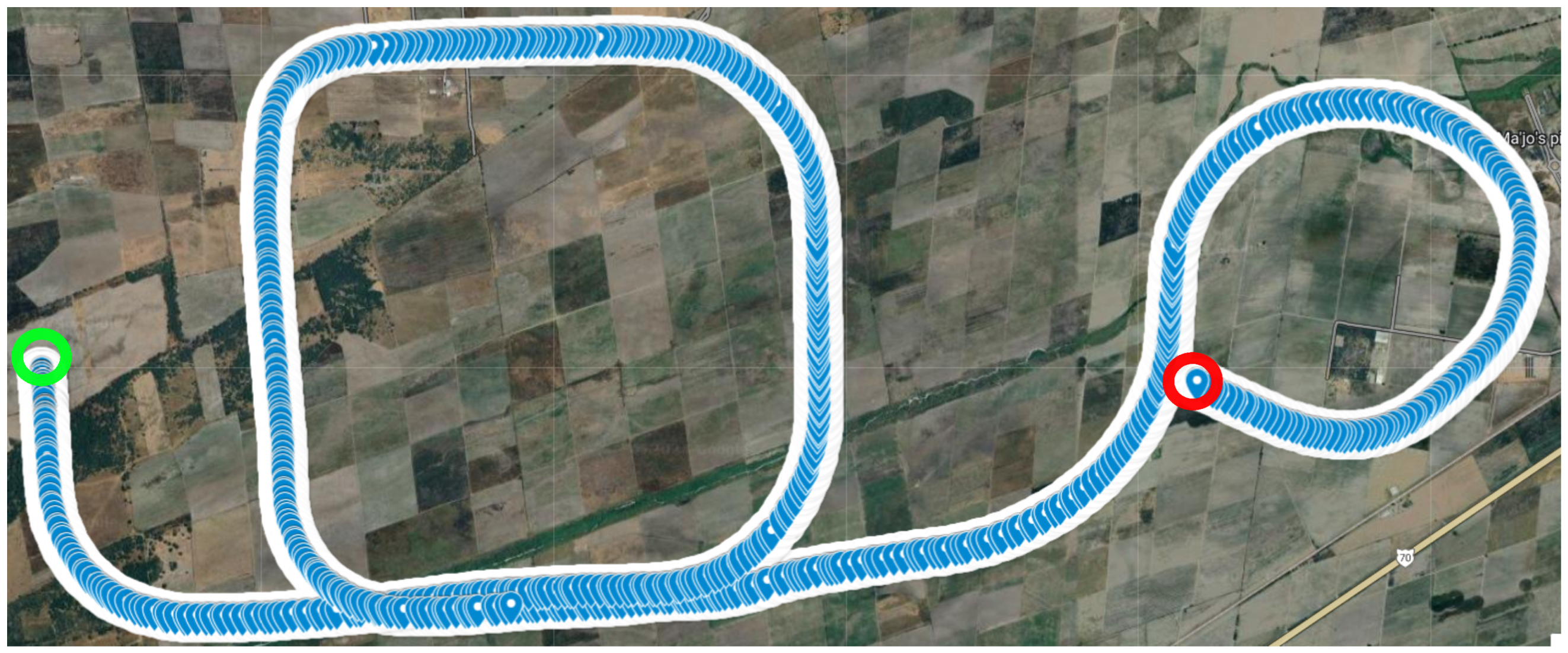
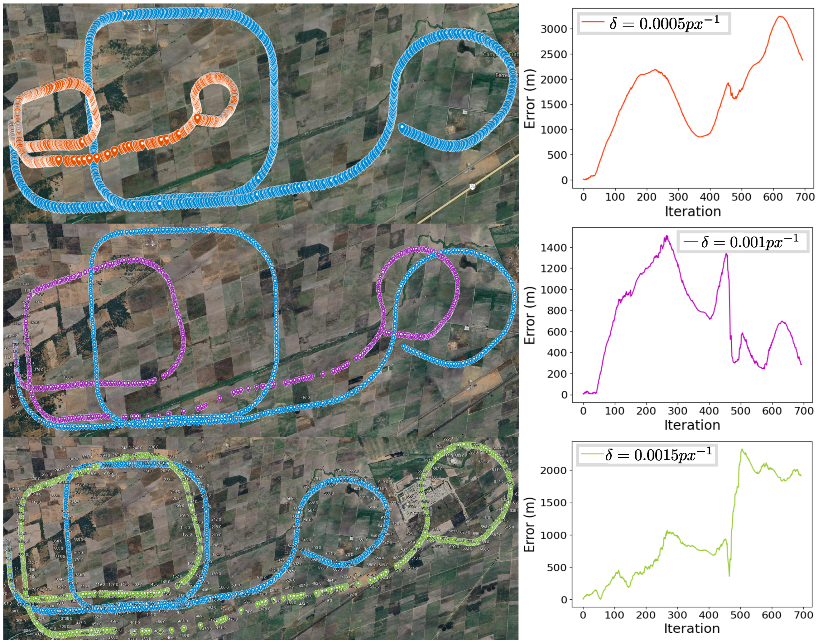
  • Visual Odometry: At the moment of GPS loss, the algorithm estimates a latitude and longitude coordinate based only on monocular vision. The accumulated error in this phase will depend on the precision with which the scale is calculated. This phase is explained in detail in Section 3.1.
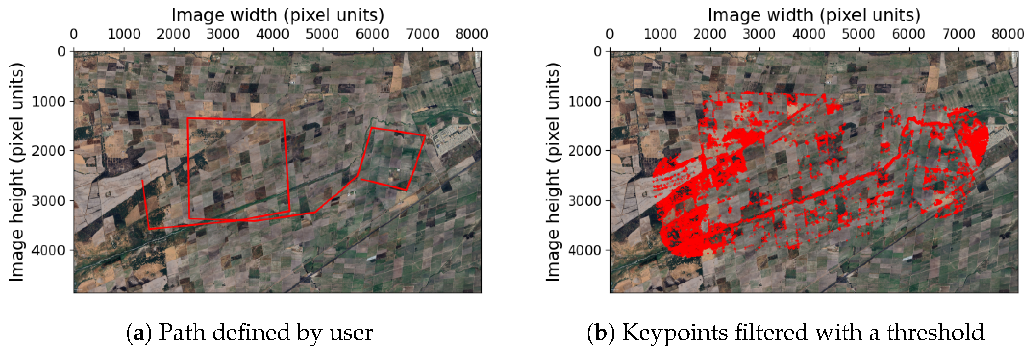
  • Satellite image preprocessing: This stage is carried out offline before the flight and is described in detail in Section 3.2. This phase is composed of the following subprocesses: We start with a flight plan, which can either be provided by the user or calculated using an exploration algorithm, in this case, Rapidly-exploring Random Trees (Section 3.2.1). From the flight plan, the keypoints of the satellite image are filtered to reduce their cardinality (Section 3.2.2). Finally, the problem of spatial indexing is solved using a Quad-tree to efficiently find the 2D points closest to the path (Section 3.2.3).
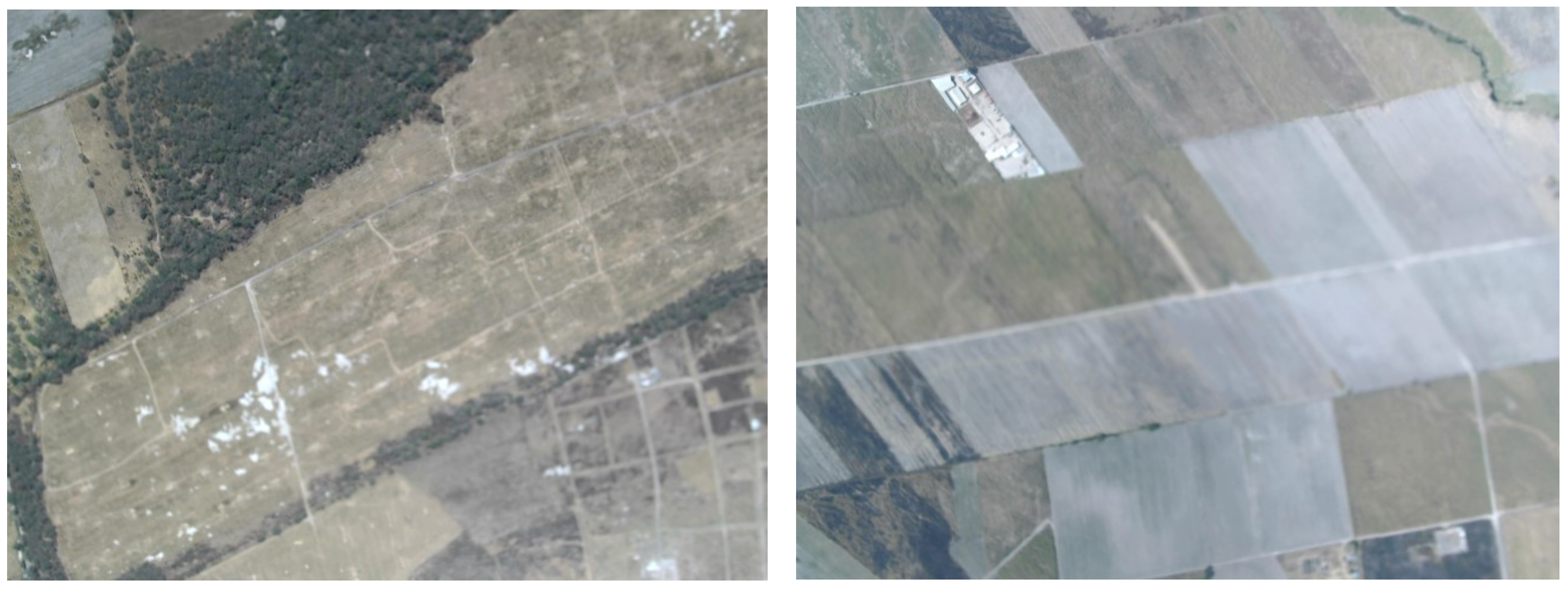
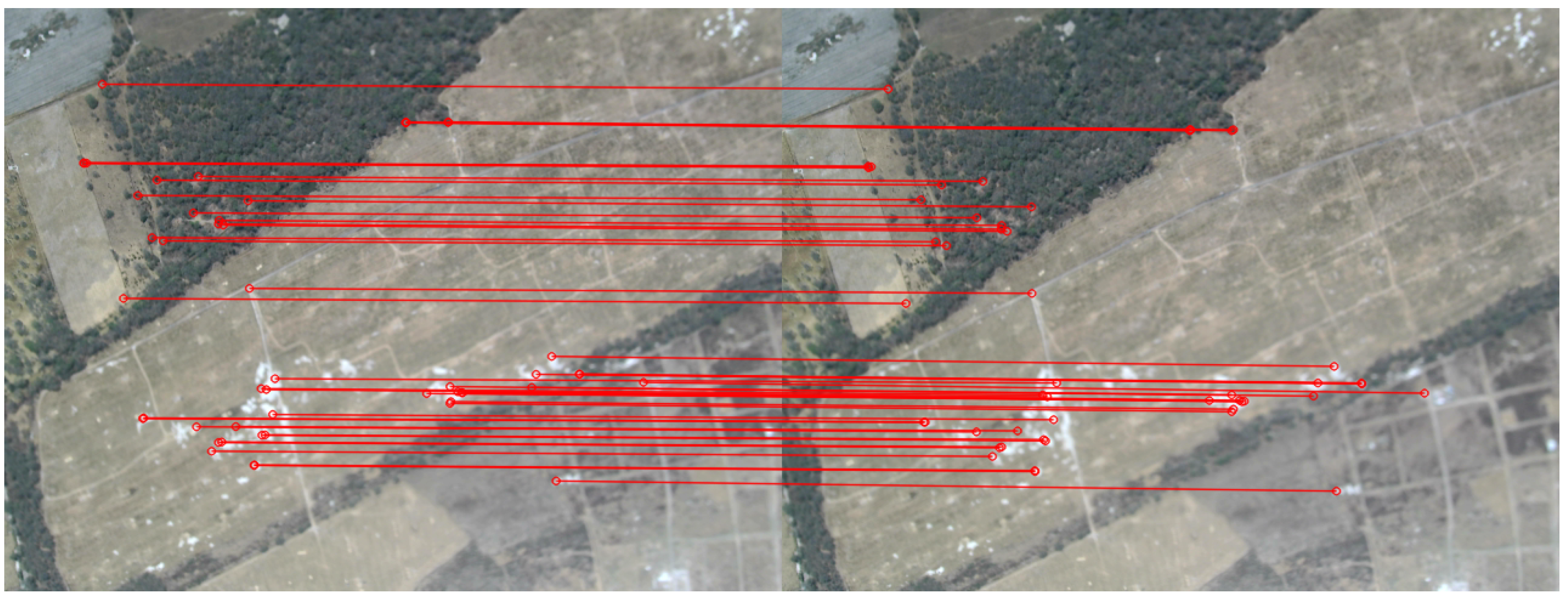
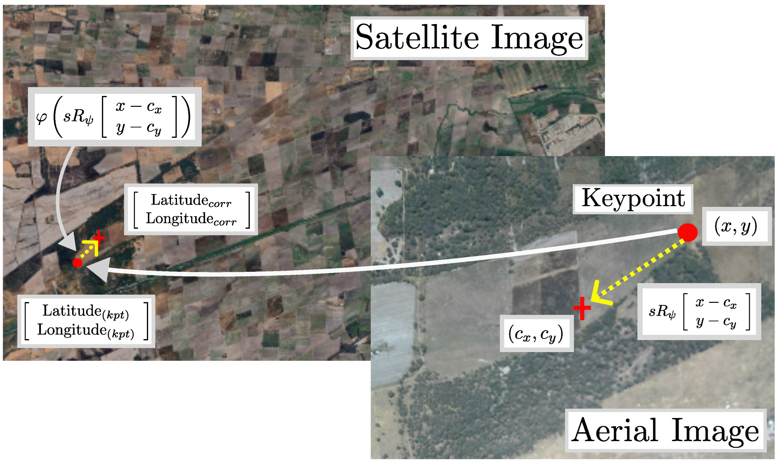
  • Reduction in accumulated error: We search for correspondences between the UAV image and the geo-referenced map to correct the estimation errors from the previous phase. The reduction error phase is explained in Section 3.3. This process is performed online and onboard the UAV.
To clarify the foundational premises and conditions of this research, as well as to define the scope and limitations of the study, we present the following assumptions.
Assumption 1.
The aircraft is equipped with a GPS signal from take off until some time after reaching the operating altitude.
Assumption 2.
The camera is always pointing towards the ground.
Assumption 3.
We have the terrain elevation map (in our case, it was obtained from the National Institute of Statistics and Geography in Mexico).
Assumption 4.
We have access to IMU and barometer data, even in the absence of GPS information.

3.1. Visual Odometry

The experiments were performed using a fixed-wing UAV flying with an altitude greater than 1000 m. Seven hundred photos were taken on a path of approximately 17.3 km. Figure 1 shows the real path obtained from the GPS. The goal of the flight plan is to be sufficiently long to ensure varying terrain elevation. Additionally, the plan includes intersections in the route to evaluate how the algorithm performs when revisiting areas it has previously encountered.
It is assumed that the UAV enters into a GPS-denied zone at the start of the path in Figure 1. When the GPS signal is lost, the plane takes the first photo at (20°38′32.136″ N, 103°49′5.307″ W). The path ends at (20°38′30.6414″ N, 103°46′28.9374″ W) and Figure 2 shows both images.
Figure 3 describes this stage of the algorithm. It starts when the UAV loses the GPS signal, and it begins to calculate the location estimation based on two consecutive images. First, features are extracted from both images using Oriented Fast (Features from Accelerated Segment Test) and Rotated Brief (Binary Robust Independent Elementary Features) (ORB) [44].
Although ORB is one of the worst descriptors in terms of scale invariance, we can assume that the scale does not change substantially between the two images, as the UAV will not change its altitude drastically during its operation. On the contrary, it is one of the algorithms that finds the largest number of keypoints and is also one of the fastest. That is why we chose ORB over the other options for this phase. An analysis of different descriptor algorithms can be found in [45]. The descriptors analyzed in this study include the following:
  • Oriented Fast and Rotated Brief (ORB) [44].
  • Binary Robust Invariant Scalable Keypoints (BRISK) [46].
  • KAZE Features (KAZE) [47].
  • Accelerated KAZE (AKAZE) [48].
  • Speeded-Up Robust Features (SURF) [49].
  • Scale-Invariant Feature Transform (SIFT) [50].
The issue with detecting so many keypoints is the time it will take to establish correspondences between the images. To avoid processing all of them, we will only use matches with the shortest distance. This distance is the Hamming distance, a measure of the feature point similarity used to match binary descriptors, which we will denote by ρ .
The first step is to consider the first two consecutive images and extract the ORB features. We filter these matches to keep only the best ones. The best matches will be those whose similarity distance ρ between features is less than a threshold. This threshold will depend on the images and the descriptor algorithm used. The heuristic used for this process is as follows: a test is conducted by plotting the best 200 matches sorted by similarity ρ , and the result is shown in Figure 4. This means that there are no matching errors among the best 200 matches.
In this experiment, the similarity distance for the worst match (among the best 200 matches) is 691. Therefore, we set a threshold of 300 to ensure that we only include good matches and the output is shown in Figure 5. Although we could set a lower threshold, it is important to maintain sufficient keypoints to prevent outliers from inducing errors in the estimation of rotation and translation. In [44], an analysis of threshold selection for establishing matches using ORB is presented. However, the selection of these thresholds will depend on the application [51].
Once we know the correspondence between both point clouds, we compute their centroid:
C i = 1 n j = 1 n x i j , 1 n j = 1 n y i j
where C i is the centroid of the 2D points in the image i, x, and y are the pixel coordinates of the feature j in image i, and n is the number of good matches.
Then, we determine the optimal rotation between points, taking them to the origin and applying Singular Value Decomposition (SVD) [52,53], as follows:
H = ( q 1 i C 1 ) ( q 2 i C 2 ) T
[ U , S , V ] = SVD ( H )
R = V U T
where q j i are the coordinates of point i from the point cloud j.
Now, it is possible to find the translation d ( p x ) with
d ( p x ) = C 1 R C 2
For more detailed information on this algorithm and a full derivation of finding the optimal rotation and translation between point clouds, we recommend [52,53].
The goal is to determine the UAV movement by measuring the displacement from one point cloud to the next. It is important to note that we have access to the angle of rotation since this is information obtained from the IMU and it is available even if the GPS has been corrupted. It then involves converting the displacement of the point clouds, measured in pixel units, into the UAV displacement in meters.
There is an issue of ambiguity when trying to convert from pixels to meters. It may be true that a large displacement between the centroids is due to either moving very fast or having the keypoints very close to the UAV. Since the altitude (estimated using the barometer) is another piece of information we have access to even without GPS, we use the barometer to heuristically scale s the altitude and use this value to convert from pixel units to meters. The scale s is calculated with
s = h δ
where s is the scale to transform from pixel to meters. δ is a correction factor that has been determined by running the algorithm (using only visual odometry) and reducing the error with respect to the GPS route, and h represents the distance from the UAV to the ground. This is
h = a e
where a is the UAV altitude and e is the terrain elevation, taken from the Digital Elevation Model (DEM), which is displayed in Figure 6.
Since we are calculating a relationship between image pixels and meters, it is necessary to convert the GPS coordinates into a system that uses meters as the unit of measurement, such as UTM. This is done using the open-source Geospatial Data Abstraction Library (GDAL), which is a library used to work with geospatial data formats. We start from the last coordinates obtained from GPS (before it has been denied) and convert them to UTM coordinates. In the UTM system, the Earth is divided into 60 longitudinal zones, each spanning 6 degrees of longitude. These zones are numbered consecutively from west to east, starting at 180°W. Each zone is designated by a number from 1 to 60. Within each zone, a Transverse Mercator projection is used. This means that the surface of the earth is projected onto a cylinder that is tangent along a meridian within the zone.
UTM coordinates are typically referenced to a specific geodetic datum, such as WGS84 (World Geodetic System 1984), which provides a consistent reference surface for mapping. In the UTM system, locations on the surface of the earth are specified using easting and northing coordinates, measured in meters. UTM provides relatively high accuracy for mapping and navigation within a specific zone. However, the accuracy may decrease near the edges of zones due to distortion introduced by the projection. For a more detailed explanation about the UTM coordinate system, refer to [54,55,56,57].
The displacement of the UAV in meters is given by
d x ( U T M ) d y ( U T M ) = s d ( p x ) cos ψ s d ( p x ) sin ψ
where d x ( U T M ) and d y ( U T M ) represent the displacement in meters, and d ( p x ) is the displacement between the point clouds in pixel units. ψ is the yaw angle from the magnetometer of the IMU, and s is the scale.
Once we have the last real latitude/longitude coordinates in UTM (meters), we can add the displacement of the point clouds (in x and y direction), which have been already transformed into meters. Afterwards, the new UTM coordinate is converted back into latitude/longitude coordinates.
Up to this point, there are several issues raised. The first one is that the scale is calculated based on the altitude of the UAV relative to the terrain. Depending on the resolution of the elevation map and the resolution of the barometer, this scale may be computed incorrectly. If the scale is incorrect, the conversion between pixels and meters will contain an error, leading to the new coordinates being calculated based on this inaccurate scale.
The second problem is that this sequential algorithm relies on the previous location. If there was an error in the previous calculation, then we will be reading an incorrect elevation from the elevation map. If this reading is incorrect, then the scale for the next iteration will also have an error. In addition, if there are few keypoints, it is possible that we are computing the displacement based on some incorrect matches. In case the number of keypoints does not exceed a threshold, we will read the new yaw ψ from the magnetometer of the IMU, which is the distance between point clouds d ( p x ) that we obtained in the previous iteration (Figure 3).
Figure 7 shows the behavior of the algorithm using different values of δ to compute (6).
As expected, due to the irregularity of the terrain involved in the mission of more than 17 km, there is no single optimal value for the constant δ that is suitable for all flight segments. In Figure 7, it can be seen that δ only escalates the same shape, which does not correspond with the actual GPS reading.

3.2. Satellite Image Preprocessing

So far, the presented algorithm is able to estimate the UAV location, but the prediction error accumulates over time. To address this issue, we introduce a novel algorithm based on satellite images (geo-referenced) and the flight plan.
Using satellite imaging for localization has been explored before [58,59,60]. In [58], the authors proposed a method to index ortho-map databases by image features, facilitating the rapid search of geo-referenced images. Conversely, ref. [59] introduces an adaptation of the Cross-View Matching Network (CVM-Net) tailored for aerial imaging, which includes a Markov localization framework to ensure temporal consistency. Finally, ref. [60] presents a localization approach for multirotor drones that employs an autoencoder to map images into an embedding space, enabling image comparison using an inner product kernel.
Although the above-mentioned projects successfully achieve localization for their intended tasks, they are not suitable for a tactical fixed-wing UAV that can navigate up to 200 km. In the presented case, we have the following limitations:
  • Power consumption of the hardware: We are limited to using small, low-power hardware such as the Raspberry Pi 4 [61] or the Orange Pi 5 [62] to avoid overloading the system. This constraint means we cannot use many advanced techniques that rely on deep learning.
  • Onboard processing: In areas without GPS coverage, communication can be unreliable or nonexistent. As a result, the UAV must be capable of performing GPS estimation on board.
  • Altitude estimation: While low-altitude multirotors can achieve high precision with laser or ultrasonic sensors, in our case, we would require expensive LiDAR equipment that exceeds the payload capacity of the vehicle. In our situation, we estimate the altitude using a barometer, which can introduce errors of up to several hundred meters.
  • High-range missions: Tactical UAVs can operate over distances of up to 200 km. Therefore, the algorithms used must be able to handle long-duration flights.
To reduce the cumulative error in an efficient way, we present the following preprocessing scheme (Figure 8); we detail this scheme in the following subsections.

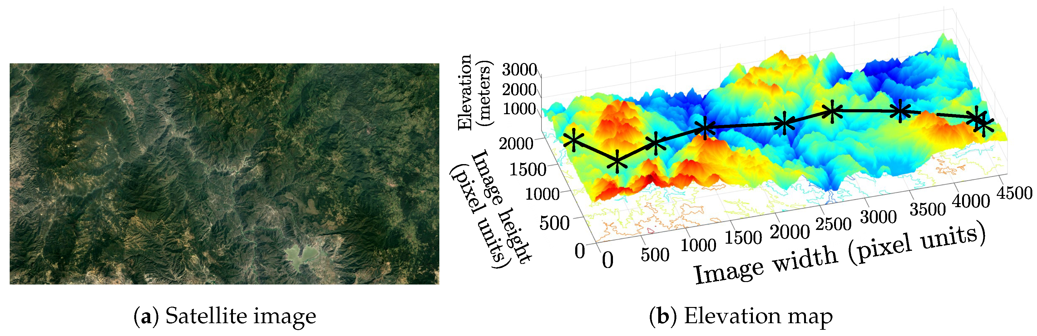
3.2.1. Calculate Flight Plan

We provide the user with two options: they can either upload a previous flight plan (a list of latitude/longitude coordinates), or we can calculate a flight plan based on the elevation map, a starting point, an end point, and a working altitude. Firstly, we load the elevation map as an image and operate this image to calculate the safe zone based on the working altitude of the plane.
We then employ Rapidly-exploring Random Tree (RRT*, with the ’*’ indicating that the algorithm is admissible, ensures that it will eventually find the shortest path as the number of samples increases) [63] to determine coordinates on the map that avoid terrain collisions. An RRT* is a random algorithm that generates random extensions from the start point. It can be applied in non-structured environments if we can calculate intersections between a known point and a newly generated point.
In Figure 9a, we show a map of a mountainous area in Hidalgo, Mexico. For better understanding, we include in Figure 9b an example of the RRT* drawn in 3D for the same map.

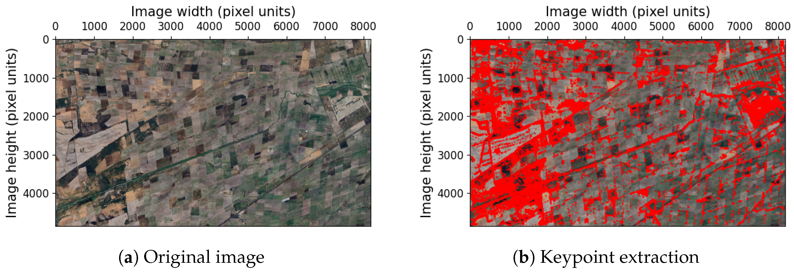
3.2.2. Filter Keypoints with the Flight Plan

Using a satellite image to reduce the accumulative error can be time-consuming. To avoid this, we apply a keypoint filter based on the flight plan. First, we calculate the keypoints from a high-resolution image. Although this process is very time-consuming, it is performed offline before the aircraft departs.
In contrast with the previous stage, where we used ORB, we are now implementing AKAZE [48] for feature extraction, which is an accelerated version of KAZE [47]. The reason for this choice is that AKAZE exhibits one of the best rotation invariances in contrast with other descriptors [45]. This is important because the photographs captured by the UAV may have orientations that differ significantly from those of the satellite image. The result of implementing AKAZE is shown in Figure 10.
The cardinality of the keypoints in Figure 10b is 68,061; this will imply a huge consumption of resources. To mitigate this, we filter these keypoints by using the flight plan that we show in Figure 11a. In this case, the user provides a path instead of calculating it.
We calculate the angular distance d α of each keypoint in the satellite image to the interpolated flight plan path with (9), where ( l a t k p , l o n k p ) represents the keypoint position on the map and ( l a t p a t h , l o n p a t h ) is the closest point to the keypoint in the flight plan path.
d α = ( l a t p a t h l a t k p ) 2 + ( l o n p a t h l o n k p ) 2
In Figure 12a, we construct the histogram of the angular distance for all the keypoints of the satellite image. This histogram is important because it gives us an idea of the keypoint distribution. The keypoints closer to the path are more likely to be good reset points.
To preserve the points closer to the path, let us set a threshold of 0.005 over the distance to the path; we can obtain the filter keypoints (Figure 11b). In this case, we count 25,256 keypoints, which is still a huge dataset to operate in real time. Notice that the resulting map is dense, expensive in memory, and does not allow us to use points far from the path to correct the error. For this reason, using a threshold on the distance does not work for this application.
To have a better filter over the keypoints, we fit an exponential probability model, shown in (10), to the histogram of the angular distance by using the maximum likelihood estimation (MLE) algorithm. In Figure 12b, we show the fitted exponential function.
f ( x ) = λ e λ x
We use the fitted exponential function to randomly sample keypoints (without replacement), where the keypoints closer to the flight plan are more likely to be sampled. This process has the advantage of allowing us to specify the number of filtered keypoints, thereby controlling the time required for correction.
In Figure 13a, we illustrate a simulation of the probability distribution over the map. Notice that the probability of using a particular site depends on this probability function and the quantity of keypoints. In Figure 13b, we present the final filtered keypoints, limited to 5000 (we have chosen this number of keypoints so that the onboard computer can process them in real time). We find that this number of keypoints allows us to achieve real-time application.

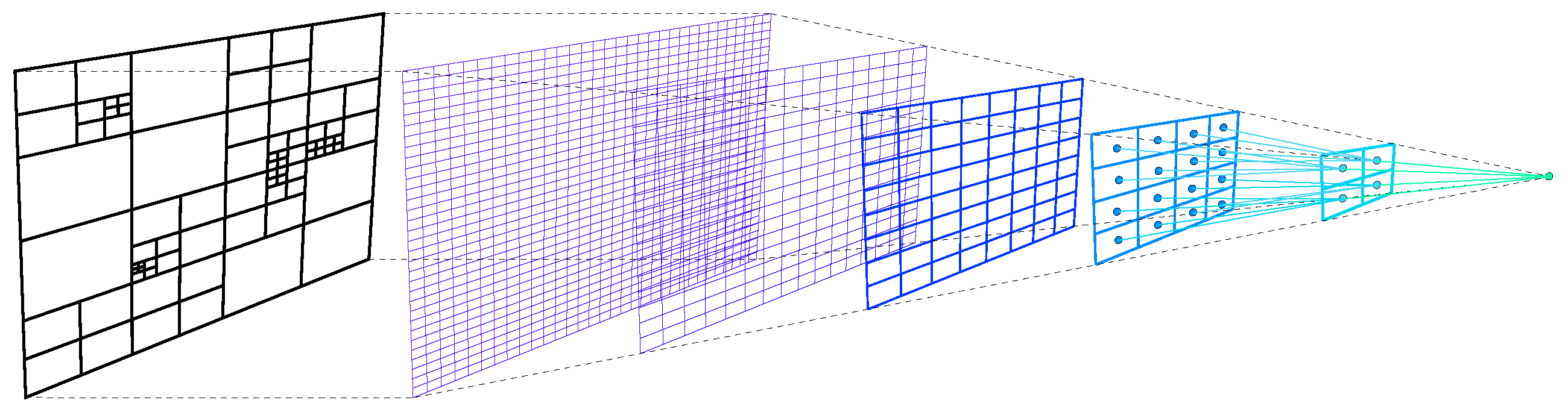
3.2.3. Spatial Indexing

Once we obtain the filtered points, we want to efficiently calculate the closest point to the current position of the plane. Comparing the current position of the UAV with each possible satellite keypoint is an O ( n ) algorithm. This can be inefficient for real-time applications.
The problem of rapidly finding 2D or 3D points near a target point is known as spatial indexing [64]. This is a highly studied problem and there are some efficient solutions like the K-dimensional tree (KD-tree) [65], Geohash [66], and Quad-tree [67]. In this paper, we implemented Quad-tree to efficiently obtain the K-nearest neighbors to search for a good match to reset the position.
In Figure 14, we offer a general scheme for the Quad-tree algorithm. As its name suggests, Quad-tree is a tree data structure in which each node has exactly four children. This allows us to search points and query the closest point in O ( l o g ( n ) ) . The tree separates a two-dimensional space into four parts, and each part can subsequently be separated into another four parts.
We have validated that Quad-tree is sufficient to archive in real time for our particular case, but we reserve a comparison with other spatial indexing techniques for future research.

3.3. Reduction in Accumulated Error
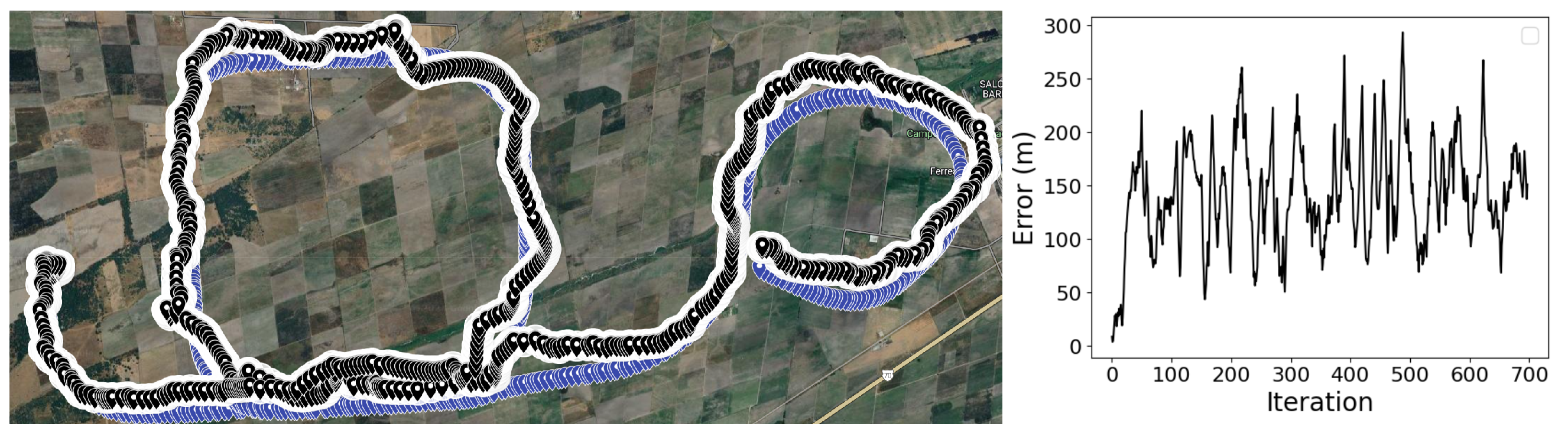
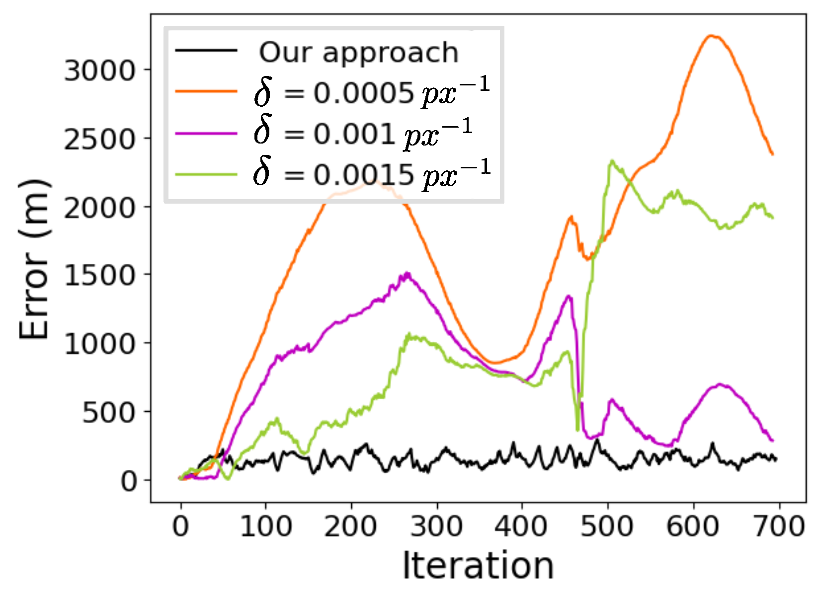
In this last stage, if we find a satellite keypoint in the current image, we use (11) to apply the coordinates correction with the offset between the keypoint in pixel coordinates and the center of the image (Figure 15). Then, we transform this offset to a latitude/longitude offset with GDAL.
Latitude c o r r Longitude c o r r = Latitude k p t Longitude k p t φ s R ψ x c x y c y
where Latitude k p t and Longitude k p t are the keypoint coordinates in the satellite image. x and y are the keypoint coordinates in the image. c x and c y are the image center. ψ is the yaw orientation, R ψ is the rotation matrix, s the scale, and φ · is the transformation from UTM to latitude/longitude.
Figure 16 is utilized to provide a concise overview of this algorithm. There is a preprocessing step where we obtain the keypoints from the satellite image. If, during the flight, we find one of these keypoints, we correct our geolocalization, otherwise, we estimate the coordinates with the visual odometry phase.

4. Results

Figure 17 shows the results of the correction algorithm. As can be seen, the error is not incremental in contrast with the previous approach, where only visual odometry was used.
Since the output is very noisy, it is decided to filter it with a Kalman Filter, and the output is shown in Figure 18.
Finally, in Figure 19, we show the errors of the visual odometry phase (the same errors shown in Figure 7) and compare them with the error plot of our approach. It can be seen that our approach prevents an increase in the error.
Based on the information from the graphs in Figure 19, we constructed Table 2. Although the accumulated error is high, this is because we summed all the errors over more than 17 km of flight. However, the average error in our algorithm is less than 150 m, which is acceptable for missions with long routes as it represents less than 1% of the error. Moreover, it has been demonstrated that the error does not accumulate.

5. Discussion

It is important to mention that this work is intended to be executed online and onboard the vehicle, and we aim for it to be computationally efficient. Therefore, given that the displacements between the images are small, we can assume that the rotations between consecutive images will not be very large and we can estimate the displacement d p x simply by the difference between the centroids C i , rather than using the SVD approach to compute the optimal rotation and translation. If this solution is chosen, it is important to threshold the correspondence distance to reduce the possibility of encountering outliers. This distance is the Hamming distance between the descriptor vectors, and a threshold below 64 is recommended [44].
Consistent with this, it is also assumed that the camera is always pointing downward. Although this is not always the case due to the UAV turning, most of the time, the homography matrix (which considers the yaw, pitch, and roll of the aircraft) with which we should transform the photographs is close to the identity matrix. Any errors that could accumulate from omitting it will be corrected each time we find a keypoint in the satellite image.
Although it is not the first time that the idea of reducing the accumulated error using reference images has been used, the field of application is different from the rest of the cited works. In our case, it involves tactical UAVs with ranges of up to 200 km at altitudes up to 3000 m flying in GPS-denied areas. In this work, errors of less than 150 m have been achieved. Although this might seem like a large error, within this framework (flying at more than 1000 m above the terrain and for more than 17 km without GPS coordinates), it is an acceptable error for this type of mission.
With a mean error of 142.88 m, it raises the question of whether it would be better to use a technique based solely on images and the IMU. Besides needing the dynamic model, it has been observed that even in shorter flights (2400 m range over 60 s without GPS), errors exceeding 200 m have been recorded [25], which represents an error of 8.7%. Another study that has demonstrated IMU drift is [26]. Another example is provided by [68], where a fixed-wing UAV is used. They report a 40 m drift in a test lasting 70 s at an altitude of 70 m, resulting in an error of nearly 8%. In contrast, our approach, which uses visual odometry and correction based on satellite images, has achieved an error rate of 0.83%.
Table 3 provides a summary of the reported errors in techniques with case studies comparable to ours, including visual odometry and visual–inertial techniques.

6. Conclusions

In this work, an algorithm that estimates the geolocation of a UAV in the absence of a GPS signal was presented. Several factors impact this problem, such as the altitude of the UAV relative to the terrain, the geolocation where the experiment takes place, and the distance of the route. It was demonstrated that there is no way to optimize the scale for pixel-to-meter transformation, so the error will accumulate as the aircraft moves forward. The results show that it is feasible to use satellite image features to extract landmarks that help the UAV estimate its location, even though the images are not updated and have different intensity levels and varying resolutions.
The algorithm filters the keypoints detected in the satellite image to ensure computational lightness and onboard execution capability to ensure autonomy.
It is demonstrated that this scheme prevents the error from incrementing over time even in long-range missions.

Author Contributions

Conceptualization, J.G.-A. and C.V.; methodology, C.V.; software, J.G.-A., C.V. and P.M.-R.; validation, N.A.-D.; formal analysis, C.V.; investigation, P.M.-R.; data curation, J.G.-A.; writing—original draft preparation, J.G.-A. and C.V.; writing—review and editing, N.A.-D.; visualization, P.M.-R.; supervision, J.G.-A.; project administration, J.G.-A. and C.V. All authors have read and agreed to the published version of the manuscript.

Funding

This research was funded by the University of Guadalajara through “Programa de Fortalecimiento de Institutos, Centro y Laboratorios de Investigación 2024”.

Institutional Review Board Statement

Not applicable.

Informed Consent Statement

Not applicable.

Data Availability Statement

The data presented in this study are available on request from the corresponding author. The data are not publicly available due to privacy.

Conflicts of Interest

The authors declare no conflicts of interest. The funders had no role in the design of the study; in the collection, analyses, or interpretation of the data; in the writing of the manuscript; or in the decision to publish the results.

Abbreviations

The following abbreviations are used in this manuscript:
BVLOSBeyond Visual Line of Sight
DEMDigital Elevation Model
GCSGround Control Station
GDALGeospatial Data Abstraction Library
GPSGlobal Positioning System
HALEHigh-Altitude Long-Endurance
IMUInertial Measurement Unit
INSInertial Navigation System
LIDARLight Detection And Ranging
LSTMLong Short-Term Memory
MALEMedium-Altitude Long-Endurance
ORBOriented Fast and Rotated Brief
RNNRecurrent Neural Network
SVDSingular Value Decomposition
UAVUnmanned Aerial Vehicle
UGSUnattended Ground Sensor
UTMUniversal Transverse Mercator
SLAMSimultaneous Localization And Mapping
VLOSVisual Line Of Sight
VTOLVertical Take Off and Landing

References

  1. Radoglou-Grammatikis, P.; Sarigiannidis, P.; Lagkas, T.; Moscholios, I. A compilation of UAV applications for precision agriculture. Comput. Netw. 2020, 172, 107148. [Google Scholar] [CrossRef]
  2. Van den Bergh, B.; Pollin, S. Keeping UAVs under control during GPS jamming. IEEE Syst. J. 2018, 13, 2010–2021. [Google Scholar] [CrossRef]
  3. Grayson, B.; Penna, N.T.; Mills, J.P.; Grant, D.S. GPS precise point positioning for UAV photogrammetry. Photogramm. Rec. 2018, 33, 427–447. [Google Scholar] [CrossRef]
  4. Gutiérrez, G.; Searcy, M.T. Introduction to the UAV special edition. SAA Archaeol. Rec. Spec. Issue Drones Archaeol. 2016, 16, 6–9. [Google Scholar]
  5. Muchiri, G.; Kimathi, S. A review of applications and potential applications of UAV. In Proceedings of the Sustainable Research and Innovation Conference, Pretoria, South Africa, 20–24 June 2022; pp. 280–283. [Google Scholar]
  6. Ozdemir, U.; Aktas, Y.O.; Vuruskan, A.; Dereli, Y.; Tarhan, A.F.; Demirbag, K.; Erdem, A.; Kalaycioglu, G.D.; Ozkol, I.; Inalhan, G. Design of a commercial hybrid VTOL UAV system. J. Intell. Robot. Syst. 2014, 74, 371–393. [Google Scholar] [CrossRef]
  7. U.S. Army Unmanned Aircraft Systems Center of Excellence. U.S. Army Unmanned Aircraft Systems Roadmap 2010–2035: Eyes of the Army; U.S. Army Unmanned Aircraft Systems Center of Excellence: Fort Rucker, AL, USA, 2010. [Google Scholar]
  8. Davies, L.; Bolam, R.C.; Vagapov, Y.; Anuchin, A. Review of unmanned aircraft system technologies to enable beyond visual line of sight (BVLOS) operations. In Proceedings of the 2018 X International conference on electrical power drive systems (ICEPDS), Novocherkassk, Russia, 3–6 October 2018; IEEE: Piscataway, NJ, USA, 2018; pp. 1–6. [Google Scholar]
  9. Roos, J.C.J.C. Autonomous Take-Off and Landing of a Fixed Wing Unmanned Aerial Vehicle. Ph.D. Thesis, Stellenbosch University, Stellenbosch, South Africa, 2007. [Google Scholar]
  10. Qu, Y.; Zhang, Y. Cooperative localization of low-cost UAV using relative range measurements in multi-UAV flight. In Proceedings of the AIAA Guidance, Navigation, and Control Conference, Toronto, ON, Canada, 2–5 August 2010; p. 8187. [Google Scholar]
  11. Chakraborty, A.; Taylor, C.N.; Sharma, R.; Brink, K.M. Cooperative localization for fixed wing unmanned aerial vehicles. In Proceedings of the 2016 IEEE/ION Position, Location and Navigation Symposium (PLANS), Savannah, GA, USA, 11–14 April 2016; IEEE: Piscataway, NJ, USA, 2016; pp. 106–117. [Google Scholar]
  12. Iyidir, B.; Ozkazanc, Y. Jamming of GPS receivers. In Proceedings of the IEEE 12th Signal Processing and Communications Applications Conference, Kusadasi, Turkey, 30 April 2004; IEEE: Piscataway, NJ, USA, 2004; pp. 747–750. [Google Scholar]
  13. Navigation, T.R.; Foundation, T. Prioritizing Dangers to the United States from Threats to GPS: Ranking Risks and Proposed Mitigations. Available online: https://rntfnd.org/wp-content/uploads/12-7-Prioritizing-Dangers-to-US-fm-Threats-to-GPS-RNTFoundation.pdf (accessed on 13 August 2024).
  14. Borio, D.; O’driscoll, C.; Fortuny, J. GNSS jammers: Effects and countermeasures. In Proceedings of the 2012 6th ESA Workshop on Satellite Navigation Technologies (Navitec 2012) & European Workshop on GNSS Signals and Signal Processing, Noordwijk, The Netherlands, 5–7 December 2012; IEEE: Piscataway, NJ, USA, 2012; pp. 1–7. [Google Scholar]
  15. Westbrook, T. Will GPS Jammers Proliferate in the smart city? Salus J. 2019, 7, 45–67. [Google Scholar]
  16. Psiaki, M.L.; O’Hanlon, B.W.; Bhatti, J.A.; Shepard, D.P.; Humphreys, T.E. GPS spoofing detection via dual-receiver correlation of military signals. IEEE Trans. Aerosp. Electron. Syst. 2013, 49, 2250–2267. [Google Scholar] [CrossRef]
  17. Manfredini, E.G.; Akos, D.M.; Chen, Y.H.; Lo, S.; Walter, T.; Enge, P. Effective GPS spoofing detection utilizing metrics from commercial receivers. In Proceedings of the 2018 International Technical Meeting of The Institute of Navigation, Reston, VA, USA, 29 January–1 February 2018; pp. 672–689. [Google Scholar]
  18. O’Hanlon, B.W.; Psiaki, M.L.; Bhatti, J.A.; Shepard, D.P.; Humphreys, T.E. Real-time GPS spoofing detection via correlation of encrypted signals. Navigation 2013, 60, 267–278. [Google Scholar] [CrossRef]
  19. Khanafseh, S.; Roshan, N.; Langel, S.; Chan, F.C.; Joerger, M.; Pervan, B. GPS spoofing detection using RAIM with INS coupling. In Proceedings of the 2014 IEEE/ION Position, Location and Navigation Symposium-PLANS 2014, Monterey, CA, USA, 5–8 May 2014; IEEE: Piscataway, NJ, USA, 2014; pp. 1232–1239. [Google Scholar]
  20. Jung, J.H.; Hong, M.Y.; Choi, H.; Yoon, J.W. An analysis of GPS spoofing attack and efficient approach to spoofing detection in PX4. IEEE Access 2024, 12, 46668–46677. [Google Scholar] [CrossRef]
  21. Chen, J.; Wang, X.; Fang, Z.; Jiang, C.; Gao, M.; Xu, Y. A Real-Time Spoofing Detection Method Using Three Low-Cost Antennas in Satellite Navigation. Electronics 2024, 13, 1134. [Google Scholar] [CrossRef]
  22. Fan, Z.; Tian, X.; Wei, S.; Shen, D.; Chen, G.; Pham, K.; Blasch, E. GASx: Explainable Artificial Intelligence For Detecting GPS Spoofing Attacks. In Proceedings of the 2024 International Technical Meeting of The Institute of Navigation, Long Beach, CA, USA, 23–25 January 2024; pp. 441–453. [Google Scholar]
  23. Rady, S.; Kandil, A.; Badreddin, E. A hybrid localization approach for UAV in GPS denied areas. In Proceedings of the 2011 IEEE/SICE International Symposium on System Integration (SII), Kyoto, Japan, 20–22 December 2011; IEEE: Piscataway, NJ, USA, 2011; pp. 1269–1274. [Google Scholar]
  24. Conte, G.; Doherty, P. An integrated UAV navigation system based on aerial image matching. In Proceedings of the 2008 IEEE Aerospace Conference, Big Sky, MT, USA, 1–8 March 2008; IEEE: Piscataway, NJ, USA, 2008; pp. 1–10. [Google Scholar]
  25. Quist, E. UAV Navigation and Radar Odometry. Ph.D. Thesis, Bringham Young University, Provo, UT, USA, 2015. [Google Scholar]
  26. Sharma, R.; Taylor, C. Cooperative navigation of MAVs in GPS denied areas. In Proceedings of the 2008 IEEE International Conference on Multisensor Fusion and Integration for Intelligent Systems, Seoul, Republic of Korea, 20–22 August 2008; IEEE: Piscataway, NJ, USA, 2008; pp. 481–486. [Google Scholar]
  27. Russell, J.S.; Ye, M.; Anderson, B.D.; Hmam, H.; Sarunic, P. Cooperative localization of a GPS-denied UAV using direction-of-arrival measurements. IEEE Trans. Aerosp. Electron. Syst. 2019, 56, 1966–1978. [Google Scholar] [CrossRef]
  28. Misra, S.; Chakraborty, A.; Sharma, R.; Brink, K. Cooperative simultaneous arrival of unmanned vehicles onto a moving target in gps-denied environment. In Proceedings of the 2018 IEEE Conference on Decision and Control (CDC), Miami Beach, FL, USA, 17–19 December 2018; IEEE: Piscataway, NJ, USA, 2018; pp. 5409–5414. [Google Scholar]
  29. Manyam, S.G.; Rathinam, S.; Darbha, S.; Casbeer, D.; Cao, Y.; Chandler, P. Gps denied uav routing with communication constraints. J. Intell. Robot. Syst. 2016, 84, 691–703. [Google Scholar] [CrossRef]
  30. Srisomboon, I.; Lee, S. Positioning and Navigation Approaches using Packet Loss-based Multilateration for UAVs in GPS-Denied Environments. IEEE Access 2024, 12, 13355–13369. [Google Scholar] [CrossRef]
  31. Griffin, B.; Fierro, R.; Palunko, I. An autonomous communications relay in GPS-denied environments via antenna diversity. J. Def. Model. Simul. 2012, 9, 33–44. [Google Scholar] [CrossRef]
  32. Zahran, S.; Mostafa, M.; Masiero, A.; Moussa, A.; Vettore, A.; El-Sheimy, N. Micro-radar and UWB aided UAV navigation in GNSS denied environment. Int. Arch. Photogramm. Remote Sens. Spat. Inf. Sci. 2018, 42, 469–476. [Google Scholar] [CrossRef]
  33. Asher, M.S.; Stafford, S.J.; Bamberger, R.J.; Rogers, A.Q.; Scheidt, D.; Chalmers, R. Radionavigation alternatives for US Army Ground Forces in GPS denied environments. In Proceedings of the 2011 International Technical Meeting of the Institute of Navigation, San Diego, CA, USA, 24–26 January 2011; Citeseer: Princeton, NJ, USA, 2011; Volume 508, p. 532. [Google Scholar]
  34. Trujillo, J.C.; Munguia, R.; Guerra, E.; Grau, A. Cooperative monocular-based SLAM for multi-UAV systems in GPS-denied environments. Sensors 2018, 18, 1351. [Google Scholar] [CrossRef] [PubMed]
  35. Radwan, A.; Tourani, A.; Bavle, H.; Voos, H.; Sanchez-Lopez, J.L. UAV-assisted Visual SLAM Generating Reconstructed 3D Scene Graphs in GPS-denied Environments. arXiv 2024, arXiv:2402.07537. [Google Scholar]
  36. Kim, J.; Sukkarieh, S. 6DoF SLAM aided GNSS/INS navigation in GNSS denied and unknown environments. Positioning 2005, 1, 120–128. [Google Scholar] [CrossRef]
  37. Kayi, A.; Erdoğan, M.; Eker, O. OPTECH HA-500 ve RIEGL LMS-Q1560 ile gerçekleştirilen LİDAR test sonuçları. Harit. Derg. 2015, 153, 42–46. [Google Scholar]
  38. Matyja, T.; Stanik, Z.; Kubik, A. Automatic correction of barometric altimeters using additional air temperature and humidity measurements. GPS Solut. 2024, 28, 40. [Google Scholar] [CrossRef]
  39. Simonetti, M.; Crespillo, O.G. Geodetic Altitude from Barometer and Weather Data for GNSS Integrity Monitoring in Aviation. Navig. J. Inst. Navig. 2024, 71, navi.637. [Google Scholar] [CrossRef]
  40. Guang, X.; Gao, Y.; Liu, P.; Li, G. IMU data and GPS position information direct fusion based on LSTM. Sensors 2021, 21, 2500. [Google Scholar] [CrossRef] [PubMed]
  41. Yol, A.; Delabarre, B.; Dame, A.; Dartois, J.E.; Marchand, E. Vision-based absolute localization for unmanned aerial vehicles. In Proceedings of the 2014 IEEE/RSJ International Conference on Intelligent Robots and Systems, Chicago, IL, USA, 14–18 September 2014; IEEE: Piscataway, NJ, USA, 2014; pp. 3429–3434. [Google Scholar]
  42. Gurgu, M.M.; Queralta, J.P.; Westerlund, T. Vision-based gnss-free localization for uavs in the wild. In Proceedings of the 2022 7th International Conference on Mechanical Engineering and Robotics Research (ICMERR), Krakow, Poland, 9–11 December 2022; IEEE: Piscataway, NJ, USA, 2022; pp. 7–12. [Google Scholar]
  43. Jurevičius, R.; Marcinkevičius, V.; Šeibokas, J. Robust GNSS-denied localization for UAV using particle filter and visual odometry. Mach. Vis. Appl. 2019, 30, 1181–1190. [Google Scholar] [CrossRef]
  44. Rublee, E.; Rabaud, V.; Konolige, K.; Bradski, G. ORB: An efficient alternative to SIFT or SURF. In Proceedings of the 2011 International Conference on Computer Vision, Barcelona, Spain, 6–13 November 2011; IEEE: Piscataway, NJ, USA, 2011; pp. 2564–2571. [Google Scholar]
  45. Tareen, S.A.K.; Saleem, Z. A comparative analysis of sift, surf, kaze, akaze, orb, and brisk. In Proceedings of the 2018 International Conference on Computing, Mathematics and Engineering Technologies (iCoMET), Sukkur, Pakistan, 3–4 March 2018; IEEE: Piscataway, NJ, USA, 2018; pp. 1–10. [Google Scholar]
  46. Leutenegger, S.; Chli, M.; Siegwart, R.Y. BRISK: Binary robust invariant scalable keypoints. In Proceedings of the 2011 International Conference on Computer Vision, Barcelona, Spain, 6–13 November 2011; IEEE: Piscataway, NJ, USA, 2011; pp. 2548–2555. [Google Scholar]
  47. Alcantarilla, P.F.; Bartoli, A.; Davison, A.J. KAZE features. In Proceedings of the Computer Vision–ECCV 2012: 12th European Conference on Computer Vision, Florence, Italy, 7–13 October 2012; Proceedings, Part VI 12. Springer: Berlin/Heidelberg, Germany, 2012; pp. 214–227. [Google Scholar]
  48. Alcantarilla, P.F.; Solutions, T. Fast explicit diffusion for accelerated features in nonlinear scale spaces. IEEE Trans. Patt. Anal. Mach. Intell. 2011, 34, 1281–1298. [Google Scholar]
  49. Bay, H.; Ess, A.; Tuytelaars, T.; Van Gool, L. Speeded-up robust features (SURF). Comput. Vis. Image Underst. 2008, 110, 346–359. [Google Scholar] [CrossRef]
  50. Lowe, D.G. Distinctive image features from scale-invariant keypoints. Int. J. Comput. Vis. 2004, 60, 91–110. [Google Scholar] [CrossRef]
  51. Weberruss, J.; Kleeman, L.; Drummond, T. ORB feature extraction and matching in hardware. In Proceedings of the Australasian Conference on Robotics and Automation, Canberra, Australia, 2–4 December 2015; pp. 2–4. [Google Scholar]
  52. Arun, K.S.; Huang, T.S.; Blostein, S.D. Least-squares fitting of two 3-D point sets. IEEE Trans. Pattern Anal. Mach. Intell. 1987, PAMI-9, 698–700. [Google Scholar] [CrossRef]
  53. Sorkine-Hornung, O.; Rabinovich, M. Least-squares rigid motion using svd. Computing 2017, 1, 1–5. [Google Scholar]
  54. Fernández-Coppel, I.A. La Proyección UTM. In Área de Ingeniería Cartográfica, Geodesia y Fotogrametría, Departamento de Ingeniería Agrícola y Forestal, Escuela Técnica Superior de Ingenierías Agrarias, Palencia; Universidad de Valladolid: Valladolid, Spain, 2001. [Google Scholar]
  55. Franco, A.R. Características de las Coordenadas UTM y Descripción de Este Tipo de Coordenadas. 1999. Available online: http://www.elgps.com/documentos/utm/coordenadas_utm.html (accessed on 12 August 2024).
  56. Langley, R.B. The UTM grid system. GPS World 1998, 9, 46–50. [Google Scholar]
  57. Dana, P.H. Coordinate systems overview. In The Geographer’s Craft Project, Department of Geography, The University of Colorado at Boulder; Available online: https://foote.geography.uconn.edu/gcraft/notes/coordsys/coordsys_f.html (accessed on 13 August 2024).
  58. Wu, C.; Fraundorfer, F.; Frahm, J.M.; Snoeyink, J.; Pollefeys, M. Image localization in satellite imagery with feature-based indexing. In Proceedings of the XXIst ISPRS Congress: Technical Commission III. ISPRS, Beijing, China, 3–11 July 2008; Volume 37, pp. 197–202. [Google Scholar]
  59. Hu, S.; Lee, G.H. Image-based geo-localization using satellite imagery. Int. J. Comput. Vis. 2020, 128, 1205–1219. [Google Scholar] [CrossRef]
  60. Bianchi, M.; Barfoot, T.D. UAV localization using autoencoded satellite images. IEEE Robot. Autom. Lett. 2021, 6, 1761–1768. [Google Scholar] [CrossRef]
  61. Gay, W. Raspberry Pi Hardware Reference; Apress: New York, NY, USA, 2014. [Google Scholar]
  62. Orange Pi 5 plus User Manual. Available online: https://agelectronica.lat/pdfs/textos/O/ORANGEPLUS5GB.PDF (accessed on 13 August 2024).
  63. Noreen, I.; Khan, A.; Habib, Z. A comparison of RRT, RRT* and RRT*-smart path planning algorithms. Int. J. Comput. Sci. Netw. Secur. (IJCSNS) 2016, 16, 20. [Google Scholar]
  64. Begum, S.A.N.; Supreethi, K. A survey on spatial indexing. J. Web Dev. Web Des. 2018, 3, 1–25. [Google Scholar]
  65. Ram, P.; Sinha, K. Revisiting kd-tree for nearest neighbor search. In Proceedings of the 25th ACM Sigkdd International Conference on Knowledge Discovery & Data Mining, Anchorage, AK, USA, 4–8 August 2019; pp. 1378–1388. [Google Scholar]
  66. Huang, K.; Li, G.; Wang, J. Rapid retrieval strategy for massive remote sensing metadata based on GeoHash coding. Remote Sens. Lett. 2018, 9, 1070–1078. [Google Scholar] [CrossRef]
  67. Tobler, W.; Chen, Z.t. A quadtree for global information storage. Geogr. Anal. 1986, 18, 360–371. [Google Scholar] [CrossRef]
  68. Ready, B.B.; Taylor, C.N. Inertially aided visual odometry for miniature air vehicles in gps-denied environments. J. Intell. Robot. Syst. 2009, 55, 203–221. [Google Scholar] [CrossRef]
  69. Ellingson, G.; Brink, K.; McLain, T. Relative visual-inertial odometry for fixed-wing aircraft in GPS-denied environments. In Proceedings of the 2018 IEEE/ION Position, Location and Navigation Symposium (PLANS), Monterey, CA, USA, 23–26 April 2018; IEEE: Piscataway, NJ, USA, 2018; pp. 786–792. [Google Scholar]
  70. McConville, A.; Bose, L.; Clarke, R.; Mayol-Cuevas, W.; Chen, J.; Greatwood, C.; Carey, S.; Dudek, P.; Richardson, T. Visual odometry using pixel processor arrays for unmanned aerial systems in gps denied environments. Front. Robot. AI 2020, 7, 126. [Google Scholar] [CrossRef]
  71. Sharifi, M.; Chen, X.; Pretty, C.G. Experimental study on using visual odometry for navigation in outdoor GPS-denied environments. In Proceedings of the 2016 12th IEEE/ASME International Conference on Mechatronic and Embedded Systems and Applications (MESA), Auckland, New Zealand, 29–31 August 2016; IEEE: Piscataway, NJ, USA, 2016; pp. 1–5. [Google Scholar]
Figure 1. The blue path represents the Ground Truth measured by the GPS sensor. The path starts at the green marker and ends at the red marker, measuring approximately 18 km. We used Google Earth to visualize the data (Google Earth is a trademark of Google LLC).
Applsci 14 07420 g001
Figure 2. First and final photo. It is assumed that GPS signal is lost when the first photo is taken and it is not restored along the entire trajectory.
Applsci 14 07420 g002
Figure 3. Flowchart of the visual odometry phase. The algorithm starts when the GPS signal is lost. The first step is to take two consecutive images and find correspondences between keypoints (represented with the red lines). Then, we calculate the displacement between the centroids of the point clouds (represented with the red dots) d ( p x ) in pixel units; these point clouds are the keypoints corresponding to the good matches. This displacement is converted to meters and added to the previous coordinate (in UTM). Finally, the result is transformed into latitude/longitude coordinates, and the process is repeated with the next image.
Applsci 14 07420 g003
Figure 4. Matches between consecutive images. The red lines connect the pixels from the first image with their corresponding ones in the second image. The figure shows the best 200 matches.
Applsci 14 07420 g004
Figure 5. Matches between consecutive images. The figure shows, with red lines, the matches between keypoints with ρ < 300 .
Applsci 14 07420 g005
Figure 6. Elevation map used for this study (Figure 1). Geodetic reference data: the datum corresponds to ITRF92 epoch 1988.0, GRS80 ellipsoid, geographic coordinates.
Applsci 14 07420 g006
Figure 7. Comparison of GPS coordinate estimation against the flight path (ground truth), represented with the blue markers, using different values ( δ = 0.0005 p x 1 , δ = 0.001 p x 1 , δ = 0.0015 p x 1 ) and its error accumulation.
Applsci 14 07420 g007
Figure 8. Preprocessing flowchart (offline preprocessing). This process ensures the best keypoints are maintained to compare the real-time application. We included images of every subprocess for a better understanding, but they are shown better in Section 3.2.1, Section 3.2.2 and Section 3.2.3.
Applsci 14 07420 g008
Figure 9. Example (3D) of RRT* path planning over a section of Hidalgo State in Mexico. We show the final path. Geodetic reference data: the datum corresponds to ITRF92 epoch 1988.0, GRS80 ellipsoid, geographic coordinates. In (b), we use a colormap to represent elevation and the ∗ symbol represent the calculated flight plan.
Applsci 14 07420 g009
Figure 10. Demonstration of the number of keypoints present in the satellite image. In the flight plan area, 68,061 keypoints have been identified, which are shown in (b).
Applsci 14 07420 g010
Figure 11. Satellite image keypoints filtered based on their proximity to the flight plan defined by the user and represented with the red line in (a).
Applsci 14 07420 g011
Figure 12. Distance histogram and its fitted exponential decay probability distribution.
Applsci 14 07420 g012
Figure 13. Map of filtered keypoints based on the flight plan.
Applsci 14 07420 g013
Figure 14. Quad-tree scheme. It divides a space into four quadrants or regions, recursively breaking down each quadrant into smaller sub-quadrants. This process continues until a specified level of detail is reached or the region contains no more than a certain number of data points [67].
Applsci 14 07420 g014
Figure 15. Offset from the keypoint to the image center. The red dots represent the matched keypoint, and the yellow dotted arrow is the offset to the the center of the image, which is marked with the red cross.
Applsci 14 07420 g015
Figure 16. Flowchart of our algorithm: The keypoints of the satellite image are computed offline. Then, during the flight, we compute the visual odometry phase and apply a correction if we find a keypoint from the satellite image.
Applsci 14 07420 g016
Figure 17. Output of the correction algorithm.
Applsci 14 07420 g017
Figure 18. Filtered output of the correction algorithm using the Kalman Filter.
Applsci 14 07420 g018
Figure 19. Filtered output of the correction algorithm.
Applsci 14 07420 g019
Table 1. UAV classification [7].
ClassCategoryOperating Altitude
(ft)
Range
(km)
Payload
(kg)
IMicro (<2 kg)<300050.2–0.5
IMini (2–20 kg)<3000250.5–10
IISmall (<150 kg)<500050–1505–50
IIITactical<10,000<20025–200
IVMedium-Altitude
Long-Endurance
(MALE)
<18,000>1000>200
VHigh-Altitude
Long-Endurance
(HALE)
>18,000>1000>200
Table 2. Error comparison in meters (m). Mission range 17,300 m.
ClassAccumulated
Error
Root Mean
Square Error
(RMSE)
Mean
Error
StdMean
Error (%)
δ = 0.00051,184,118.531893.991706.22822.209.86
δ = 0.001516,631.52845.68744.42401.274.30
δ = 0.0015696,712.031230.591003.90711.715.80
Our Approach99,732.63150.79142.8848.190.83
Table 3. Comparison with other approaches with case studies comparable to ours.
StudyRange (m)Altitude (m)Time (s)Error (%)
Quist [25]2400NA608.70
Ready and Taylor [68]50070708.0
Ellingson et al. [69]1800501603
McConville et al. [70]79054502.53
Sharifi et al. [71]80NA4501.3
Our approach17,30012006000.83
Disclaimer/Publisher’s Note: The statements, opinions and data contained in all publications are solely those of the individual author(s) and contributor(s) and not of MDPI and/or the editor(s). MDPI and/or the editor(s) disclaim responsibility for any injury to people or property resulting from any ideas, methods, instructions or products referred to in the content.

