Abstract
Multi-pitch perception is investigated in a listening test using 30 recordings of musical sounds with two tones played simultaneously, except for two gong sounds with inharmonic overtone spectra, judging roughness and separateness as the ability to tell the two tones in each recording apart. Of the sounds, 13 were from a Western guitar playing all 13 intervals in one octave, the other sounds were mainly from non-Western instruments, comparing familiar with unfamiliar instrument sounds for Western listeners. Additionally the sounds were processed in a cochlea model, transferring the mechanical basilar membrane motion into neural spikes followed by post-processing simulating different degrees of coincidence detection. Separateness perception showed a clear distinction between familiar and unfamiliar sounds, while roughness perception did not. By correlating perception with simulation different perception strategies were found. Familiar sounds correlated strongly positively with high degrees of coincidence detection, where only 3–5 periodicities were left, while unfamiliar sounds correlated with low coincidence levels. This corresponds to an attention to pitch and timbre, respectively. Additionally, separateness perception showed an opposite correlation between perception and neural correlates between familiar and unfamiliar sounds. This correlates with the perceptional finding of the distinction between familiar and unfamiliar sounds with separateness.
1. Lead Paragraph
Brain dynamics during perception is often found to happen in self-organizing neural fields rather than concentrating on single brain areas or even single neurons. Additionally, the old notion of subcortical neural structures being unconscious is challenged, especially in the auditory pathway, where pitch and timbre appear in complex neural fields, and higher cortical brain regions seem to be responsible for associative musical tasks like rhythm extraction, musical tension, and music theory. Although the field notion of perception in the auditory pathway works very well with single musical tones, complex musical intervals, chords, or polyphonic music lead to more complex behaviour due to the strong nonlinearity of the cochlea and neural networks. As the auditory pathway reduces the auditory input through coincidence detection of neurons, we investigate the process of coincidence detection of multi-pitch sounds both in a listening test as well as by cochlea and neural simulations.
2. Introduction
Multi-pitch sound consists of more than one musical tone, where each tone has a harmonic overtone spectrum constituting musical intervals, chords, or polyphonic textures [1]. Helmholtz suggested that in such cases the roughness of the sound increases, and reasoned the musical major scale to consist of such intervals with least roughness [2], which are the musical fifth, fourth, third, etc. He calculated roughness as musical beating, as amplitude modulation, when two partials are close to each other, with a maximum roughness at a partial frequency distance of 33 Hz, decreasing to zero when partials align or when they are spaced wider apart. Other roughness estimation algorithms use similar approaches. Roughness calculations built to estimate industrial noise perception often fail to estimate musical roughness (for a review see [3]).
Another feature of musical sound perception is tonal fusion [1]. A harmonic overtone spectrum consists of many partials or frequencies; still, subjects perceive only one musical pitch, which is a fusion of all partials. By contrast, inharmonic overtones are clearly separated by perception, where the single frequencies can be perceived separately. In a multi-pitch case of musical intervals or chords, trained listeners can clearly distinguish the musical notes; they separate them. Still, some multi-pitch sounds are perceived as so dense that separation is not trivial. Therefore, a certain degree of perceptual separateness exists, which is a subject of this investigation.
Multi-pitch sound has also been subjected to separation algorithms of automatic music transcription according to auditory scene analysis [4], in terms of piano roll extraction [5], voice [6,7,8] and voice extraction [9], or multi track extraction [10,11,12].
In auditory perception, pitch and timbre are clearly distinguished, where multidimensional scaling method (MDS) listening tests showed pitch to be more salient than timbre (see, e.g., [13,14,15]; for a review see [16]). Such features are also used in sonification [17]. This salience of pitch perception was interpreted as the massive presence of the pitch periodicity as interspike intervals (ISIs) in the auditory pathway over all tonotopic auditory neural channels in the presence of a sound with harmonic overtones or partials (in the literature, overtones refer to the frequencies above the fundamental frequency; alternatively, a sound consists of partials, where the fundamental is the first partial) [18]. This is caused by drop-outs of spikes at higher frequencies, therefore constituting subharmonics. All energy-transferring auditory channels constituting a field of neighbouring neurons represent pitch much more prominently than timbre, as the ISI of the fundamental periodicity is present in all such channels, while timbre periodicities only appear in some of them. This might explain the salience of pitch over timbre, which allows melodies or a musical score mainly representing pitches to be possible.
Such a field notion of perception and cognition was also suggested for Gestalt perception and the binding problem. Haken uses the mathematical framework of a synergetic computer to model brain dynamics [19]. Taking categories as feature vectors associated with fields of neighbouring neurons, he successfully models completion of only partially present Gestalts. Baars suggests a global workspace dynamics to model levels of perception and binding between all brain regions [20]. Self-organization was found to be the cause of visual binding in the cat visual cortex [21].
Global synchronization of neurons was also found to be the cause of expectancy [22]. Using an electronic dance music (EDM) piece, where by several continuous increases of instrumentation density climaxes are composed which are expected by listeners in this genre, a synchronization of many brain areas was found to peak at the climaxes, decline afterwards, and build up with the next instrumentation density increase [23].
Perception represented as spatiotemporal patterns appearing in a spatial field of neighbouring neurons has been found in the olfactory, auditory, and visual cortex [24,25]. An amplitude modulation (AM) pattern was found, where during the large amplitude phase of AM a spatiotemporal pattern is established in a neural field, which breaks down at the amplitude minimum of the AM. The patterns themselves have been shown to rotate through a large-amplitude cycle.
A similar finding was made in the A1 of the auditory cortex when training gerbils in terms of raising and falling pitches in a discrimination task [26]. Using different auditory stimuli and several training phases, a field of neighbouring neurons shows complex patterns. These patterns differ for immediate perception after a few hundred milliseconds and after about 4 s; these have been interpreted as discrimination and categorization, respectively.
Synchronization of auditory input happens at several stages in the auditory pathway. Phase alignment of frequencies in a sound with a harmonic overtone spectrum happens at the transition of mechanical waves on the basilar membrane (BM) to spikes [27]. Further synchronization is performed in the cochlear nucleus and the trapezoid body [28,29,30,31,32]. Coincidence detection neural models are able to account for spike synchronization to spike bursts up to about 300–700 Hz, depending on the neural input strength [27].
Coincidence detection is also performed through complex neural networks on many levels. In the auditory pathway, several neural loops are present, like the loop of the cochlea, cochlear nucleus, trapezoid body, and back to the basilar membrane efferents for frequency sharpening [33]. Loops also exist between the inferior culliculus or medial geniculate body to and from the auditory cortex or the cochlear nucleus to and from the superior olive complex or the inferior culliculus. In all these loops, complex coincidence mechanisms might occur.
Rhythms in the brain are manifold [34,35,36] and of complex nature. Often, interlocking patterns appear like that of the mechanical transition into spikes in the cochlea, as discussed above, or by neighbouring neurons interlocking to each other. Such mechanisms often use complex neural loops, like that from the cochlea, to the cochlear nucleus, to the trapezoid body, and back to the cochlea for increasing pitch perception. Another example is the loop from the cochlea up to the A1 of the auditory cortex and back down, where the way from A1 to the cochlea is transmitted through only one intermediate nucleus.
In all cases, interlocking leads to a sharpening of the neural spike burst where blurred bursts are temporally aligned to arrive at a more concise, single burst. This is the outcome of coincidence detection and used in the methodology discussed below.
Indeed, the cochlea seems very effectively tuned to detect mechanisms and useful information on acoustic processes of the outside world. Modern theories of effective auditory coding have been proposed using a cochlea model and correlating its output to a template modelling psychoacoustic data [37,38]. Efficient coding was found with the cat auditory nerve compromising between ambient and crackling noise using gammatones [39]. Applying this method to a single sound shows that very few gammatones are needed to code entire sounds [16]. Mechanisms for the fusion of sound into a single pitch have been proposed as autocorrelations of sounds or of common pitch denominators like residual pitch [40,41,42]. The cochlea is also able to follow acoustical bifurcations on musical instrument sounds, like the surface tone of a cello, very precisely [43].
Coincidence detection is highly interesting in terms of the musical sound production and perception cycle [43]. Musical instruments internally work by impulses travelling within the instrument which are reflected at geometrical positions and return to an initial point where they synchronize to a periodicity, and therefore, create a harmonic sound [16]. These impulse patterns are then radiated into air and reverberate or become distorted, which is the single frequencies in the sound spectrum getting out of phase. When they enter the ear and the auditory system, the desynchronized phases become aligned again through several mechanisms, of which coincidence detection is an important one. In the brain, even stronger synchronization appears towards perceptual expectation time points [44,45]. Within a framework of a Physical Culture Theory [43] an algorithm of Impulse Pattern Formulation (IPF) was proposed to model musical expectation using synchronization of coincidence-aligned spike bursts [27]. This algorithm also works for human–human interaction, modelling tempo alignment between two musicians [46].
The present study investigates the perception and neural correlates to two-tone sounds, consisting of two musical notes played by the same instrument at the same time. Such sounds are perceived with a certain amount of roughness and separateness as the ability to hear both tones separately at the same time. These perceived psychoacoustical parameters need to correlate with neural spike patterns in the auditory pathway. Still, the perception is expected to follow different strategies depending on the familiarity of musical instrument sounds. With instruments familiar to Western listeners, e.g., the guitar, pitch extraction might be an easier task compared to pitch extraction of unfamiliar sounds.
Due to the nonlinearity of the cochlea and the auditory pathway it is not expected that the pitch theory of the fundamental periodicity appearing in all energy-holding nerve fibres due to drop-outs and subharmonics can work the same with two tones as with one tone by simply adding the behaviour of each single tone together. Rather, new behaviour is expected and investigated in this paper.
We first describe the method of the listening test, spike model, and spike post-processing, simulating coincidence detection. Then, the results of both methods are discussed. Finally, the correlation between perception and calculation is presented.
3. Method
3.1. Listening Test
In a listening test, 30 musical sounds were presented to 28 subjects aged 19–42 with a mean of 24.9; 15 female and 13 male. They were students at the Institute of Systematic Musicology at the University of Hamburg; all except for five played Western musical instruments like guitar, piano, trumpet, or drums. There was only one mention of a non-Western instrument, the ukulele. Only five subjects indicated that they were trained in musical interval identification. The subjects therefore had a bias towards Western musical instruments, which is needed in the study comparing familiar (Western) and unfamiliar (non-Western) musical instrument sounds.
All sounds presented two musical tones played on real instruments (no samples used), except for two gong sounds, which were played as single gong tones. In terms of standardization, all instruments were recorded and played back to subjects using loudspeakers. Headphones were rejected as the setup is very individual and introduces a bias. The sounds were played in random order, where the same random distribution was used for all subjects.
The gong sounds consist of inharmonic overtone spectra and were used to estimate a multi-pitch perception for percussion instruments. Table 1 gives the instruments used together with the played intervals.

Table 1.
List of sounds used in analysis and listening test. The guitar sounds cover the whole range of half-tone steps in one octave. They are supposed to be familiar for Western listeners. The other sounds are nearly all from non-Western instruments, and therefore, taken to be unfamiliar for Western listeners.
To have a systematic reference for all intervals within an octave, 13 sounds were played with a Western guitar, all with lower pitch g3 and a second pitch above g3 in thirteen half-tone steps from unisono up to the octave g4. The pitches are in the middle range of guitar playing and well within singing range. These pitches were assumed to be familiar to Western listeners.
On the other hand, nearly all other sounds were from non-Western instruments like the Chinese hulusi, a free-reed wind instrument with three tubes, where two tubes were played. There is no such instrument in the West. Although the harmonica or the accordion are also free-reed instruments, the pitch of these instruments is determined by the reed. With the hulusi, on the other hand, the pitch is determined by the length of a bamboo tube the reed is attached to. Using a regular fingering technique different pitches can be played. The hulusi used was collected by the author in Lijiang, Yunnan, China.
The saung gauk is a Burmese arched harp. Its strings are attached to an arched stick on both sides, where one side of the stick is attached to a resonance box covered with ox leather, which again is covered with heavy lacquer. It is astonishingly loud for a harp, which is caused by resonance of the stick and the resonance body. For the experiment a Mong crocodile saung gauk was used, collected by the author in Yangon, Myanmar.
The roneat deik used in the experiment is a metallophone consisting of 21 metal plates collected by the author in Phnom Penh, Cambodia. Although gong ensembles are common in Southeast Asia, the roneat deik is the rare case of a metal instrument, most other are made of bronze. The sound of each plate has an inharmonic overtone spectrum, still its fundamental is strong, making it possible to play melodies with it. Still, it is expected that the sound of the instrument is unfamiliar to Western listeners.
The dutar used is a long-neck lute collected by the author in Kashgar, Xinjiang, China. It is played as a folk instrument by the Uyghur people along the traditional silk road. It has two strings, where two pitches are played at the same time. Although it is a plucked stringed instrument like the guitar, the sound is considerably different from a guitar or a lute, caused by the unusual length of the strings on a long-necked lute and the small resonance body.
The mbira is also known as a thumb piano. It consists of nine metal plates attached to a wooden resonance box. Although the spectra of the metal rods are inharmonic, the fundamental frequencies of each spectrum are much stronger in amplitude than the higher partials, and therefore, melodies can be played on the instrument. Its origin is unknown, but it was most likely built for Western musicians in the World Music scene.
The two gongs were collected by the author in Yangon, Myanmar, and are played within the hsain waing ensemble of traditional Bama music. The large gong has a diameter of 54 cm, the diameter of the small one is 26 cm.
Two other sounds were used, a piano and a synth pad sound. These sounds were created by a Kawai MP-13 keyboard. The pad sound was used as a continuous sound, which most of the other sounds were not. The piano sound was used because it is a standard instrument for musical training. Pad sounds are generally familiar to Western listeners. Still, as synth sounds can be composed by any synthesis method with any parameters, these sounds were denoted as unfamiliar. Also, the piano sounds were added to the unfamiliar sounds in the analysis. Although this is not perfectly correct, the advantage is to keep the 13 guitar sounds as a group of homogeneous sounds. There is only one piano sound in the sound set and taking it out does not change the results considerably.
Subjects were presented all sounds three times and asked to rate their perception of the sounds’ roughness and separateness, each on a scale of 1–9, where 1 is no roughness/no separateness and 9 is maximum roughness/maximum separateness. To give subjects an idea about where these maxima might be, before the test several sounds used in the test were played, which in a pretest turned out to be those perceived as most rough and separate, respectively.
Additionally, the subjects were asked to identify the musical interval of the sounds, e.g., fifth, fourth, etc. This task was optional, as it was not clear how many subjects would have the capability of identifying the intervals and those with less capacity were asked not to waste time and attention on this task. A small questionnaire asking for age, gender, and musical instrument played by the subjects was presented before the listening test. The musical interval training of the subjects was also asked for at this time, where only five subjects indicated they had intense training. Indeed, only five subjects answered some of the intervals, most of them were wrong. Therefore, in the following it is not possible to correlate correct interval identification by subjects with the other findings. Still, we can state that nearly all subjects did not have a considerable musical interval identification capability.
3.2. Cochlea Model
All sounds were processed using a cochlea model with post-processing of the cochlea output. The cochlea model has been used before in a study of phase synchronization of partials in the transition between mechanical motion on the basilar membrane into neural spikes [27], in a coincidence detection model using an Iszikevich neural model [27], when studying cello surface sounds [43], and as foundation of a pitch theory [18].
The model assumes the basilar membrane (BM) to consist of 48 nodal points and uses a finite difference time-domain (FDTD) solution with a sample frequency of 96 kHz to model the BM motion. The sample frequency is needed to ensure model stability. The recorded sounds played to the subjects were used as input to the model. The sounds had a sample rate of 96 kHz, corresponding to that of the model. The BM is driven by the ear channel pressure, which is assumed to act instantaneously on the whole BM. This is justified as the sound speed in the peri- and endolymph is about 1500 m/s, while the sound speed on the BM is only 100 m/s down to 10 m/s. The pressure acting on the BM is the input sound. The output of the BM is spike activity, where a spike is released at a maximum of the positive slope of the BM and a maximum slope in the temporal movement at one point on the BM. This results in a spike train similar to measurements.
With periodic sounds the spikes are only present at the respective Bark bands of best frequency of the periodic sound. With harmonic overtone spectra all Bark bands of the spectral components show spikes, while the other Bark bands do not. Also, the delay between the high-frequency spikes and the low frequencies at the BM apex is about 3–4 ms, consistent with experiments. The model does not add additional noise. It also has a discretization of 48 nodal points, which is two nodal points for each Bark band.
In terms of the 3–4 ms delay, it is interesting that, although the lymph is acting instantaneously on the whole basilar membrane, the wave travelling along the membrane builds up. This is the result of the inhomogeneous stiffness and damping of the basilar membrane leading to this very special kind of wave.
3.3. Post-Processing of Cochlea Model Output
The output of the cochlea model is spikes at certain time points along the BM in the Bark bands. From here the interspike intervals (ISIs) are calculated as the time interval between two spikes at one nodal point, so two for each Bark band. Accumulating the ISIs over a time interval and transforming the ISIs into frequencies like f=1/ISI, an ISI histogram of the frequency of appearance or the amplitude of certain frequencies or periodicities present in all Bark bands results.
Figure 1 gives an example of the method. At the top, an arbitrary sound file, a sawtooth wave, is used as input to the cochlea model. The model output is shown in the middle plot of spikes occurring at Bark bands displayed vertically over time; it is shown horizontally. The model output is further processed using the ISI intervals between two adjacent spikes and ordered in a histogram for each Bark band, again vertically, over time. The histogram is calculated for the time windows and a 10 cent frequency discretization.
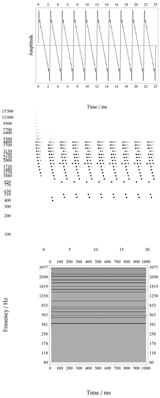
Figure 1.
Example of sound processing. Top: Sound wave. Middle: Cochlea model output of spikes in respective Bark bands (vertical axis) at respective time points (horizontal axis). Bottom: ISI histogram of occurrences of spikes with f= 1/ISI (vertical axis) over time (horizontal axis).
The accumulation interval was chosen according to logarithmic pitch perception to be 10 cent, where one octave is 1200 cent. Just-noticeable differences (JNDs) in pitch perception are frequency-dependent and strongly differ between adjacent and simultaneous sound presentation. The value of 10 cent was found to be reasonable in terms of the used sounds, where smaller values lead to too few incidences to accumulate and larger values would blur the results.
To simulate the coincidence detection found in neural nuclei subsequent to the cochlea, the ISI histograms as shown above are post-processed in three stages. First, the histograms of all time steps are summed up to build one single histogram for each sound. As shown in Figure 2 and Figure 3 the histograms change over time, mainly due to the temporal decay of the sound. They also show inharmonicities during the initial transient. After temporal integration, the ISI histogram is divided by the amplitude of its largest peak, making the amplitude of this peak one. A threshold of th = 0.01 is applied, making all peaks smaller than th zero. Additionally, all frequencies above 4 kHz are not taken into consideration, as pitch perception is only present up to this upper frequency. This is not considered a serious bias for roughness estimation as roughness, different from sharpness perception, is mainly based on low and mid-frequencies close to each other, leading to musical beatings, and therefore, to roughness. Strong energy in high frequencies is merely perceived as brightness or sharpness and does not contribute to roughness perception in the first place.
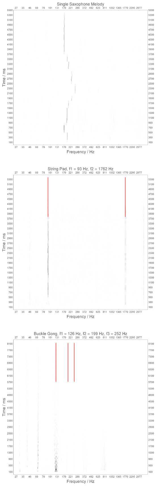
Figure 2.
Temporal development of ISI histogram, summing all ISIs in all Bark bands and transferring them into frequencies f = 1/ISI for three example sounds. Top: A single-tone saxophone melody; middle: a string pad sound consisting of two notes with fundamental frequencies Hz and Hz; bottom: a large buckle gong with three lowest frequencies Hz, Hz, and Hz. The lines at the upper part of the middle and bottom plots indicate these frequencies. The saxophone melody is perfectly represented by the strongest peak in all ISI histograms, as shown in Figure 4 in detail. The string pad’s sounds’ fundamentals are also clearly represented by the ISI histogram. The gong’s lowest partial is clearly there, still a residual ISI below this is there, too.
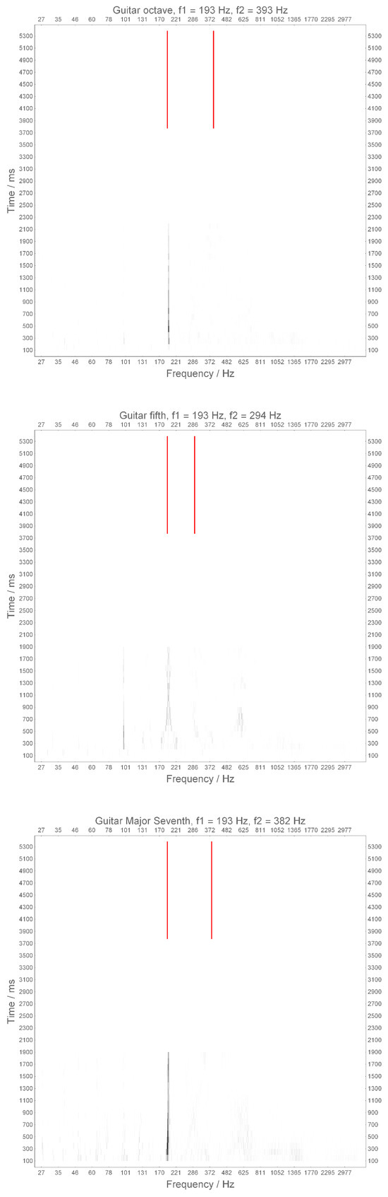
Figure 3.
Same as Figure 2 for three two-note intervals played on a classical guitar. All have the same fundamental pitch g at Hz. Top: octave above at Hz; middle: fifth above at Hz; bottom: major seventh above at Hz. In all cases, is clearly represented in the ISI histogram. With the octave the partial is nearly not present, with the fifth is again only slightly there, still a residual periodicity below appears. With the major seventh, again is nearly not present; still, many periodicities above and below are slightly present.
Secondly, Gaussian blurring of the spectrum is performed, where the spectrum is blurred using a Gauss shape with standard deviation . This sums peaks which are very close to each other, and therefore, performs coincidence detection of periodicities close to each other. As discussed in the Introduction, the very nature of coincidence detection is to make a burred neural spike temporally more concise. Therefore, using Gauss blurring allows for the detection of how concise the spike bursts are. In case of a large , coincidence is weak, as a large time interval is needed to align the peaks and vice versa. In a second step, only peaks with a certain sharpness s are used, where s = 0 selects all peaks and s > 0 selects only peaks where the negative second derivative of the spectrum is larger than s. This prevents very broad peaks still being taken as peaks after blurring of the spectrum. To estimate the amount of coincidence detection in the listening test both values are varied in 21 steps between and .
In a third step, the ISI histogram is fused into a single number to make it comparable to the judgements of separateness and roughness of the listening tests, which are also single numbers for each sound. Three methods are used: the number of peaks N, a sum of the peaks, and each weighted with its amplitude like
and a Shannon entropy like
where N is the number of peaks and ISIi is the amplitude of the ith peak.
The three methods decide which perception process is more likely to occur in listeners when correlating the results with the separateness and roughness perceptions.
3.4. Correlation Between Perception and Calculation
In a last step, the mean values for the perception of separateness and roughness, respectively, over all subjects were correlated with the results of the simulation. To address the hypothesis of different perception strategies for familiar, in this case Western, and unfamiliar instruments, the correlations were performed for two subsets of the 30 instruments. One subset consists of all 13 guitar sounds, the other subset is all other sounds. The 13 guitar sounds form a consistent set, including all 13 intervals in the octave of a Western scale. The non-Western instruments have different intervals, the two gongs consist of inharmonic spectra for comparison. In the following, the terms Western and guitar sounds, as well as non-Western and non-guitar sounds as used synonymously.
So, for each perception parameter, separateness and roughness, twelve cases exist: three summing methods N, W, and S, each for mean and standard deviation of the perception parameters, and each for the Western and non-Western subsets. Each of these twelve cases consist of 21 × 21 = 441 correlations for all combinations of and s used. For the sake of clarity, the combinations of and s are combined in one plot.
4. Results
4.1. ISI Histogram
Figure 2 and Figure 3 show six examples of ISI histograms, each consisting of adjacent time intervals, where each interval is an integration over the cochlea spike output in this interval. Five of these six examples were used in the listening test, only the top plot of Figure 2 is presented as a single-note example to exemplify the pitch theory and the salience of pitch over timbre discussed above.
This single-note example is a single-line saxophone melody. It appears that at all time intervals there is only one strong peak. Aurally, this peak follows the played melody very well. To verify this perception, in Figure 4 an excerpt of Figure 2’s top plot is shown. It shows the whole time but is restricted to the area of large peaks. The continuous curve overlaying the ISI histogram plot is the result of an autocorrelation calculation using the plain sound time series as input. With 50 ms intervals the autocorrelation of the sound time series is calculated, and the interval between the autocorrelation beginning and the first autocorrelation function peak is taken as the fundamental periodicity. This is an established method for detecting in single melodies, and has, e.g., been applied to analyse intonation of Cambodian Buddhist smot chanting [43]. Both functions, the autocorrelation and the ISI histogram, align very well. Therefore, the largest peak in the ISI histogram can be used for extraction in single melody lines.
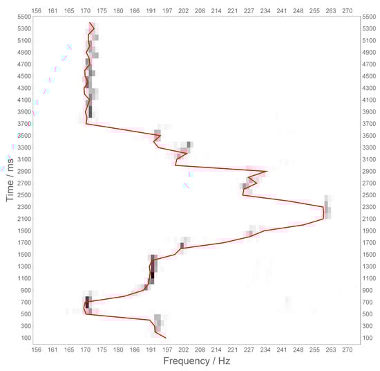
Figure 4.
Excerpt from Figure 2, top of the single saxophone line, comparing the ISI histogram temporal development with the results of an autocorrelation function of the sound’s time series when using the first peak of the autocorrelation as at adjacent time intervals. Both curves align very well. Therefore, the strongest peak of the ISI histogram represents the fundamental pitch very precisely.
Still, we are interested in multi-pitch perception. Therefore, a second example is that of a synthetic sound, a string pad, playing a two-note interval of four octaves and a major third (sound 28, f#2-a#6), with two fundamental frequencies at Hz and Hz. This sound is particularly interesting, as both pitches were perceived separately (see results of listening test below). Indeed, the two pitches are clearly represented as major peaks in the ISI histogram. In this plot, and the following, the expected peaks are indicated by solid lines starting from the top down to 0.7 of the plot’s height. The precise frequencies were calculated using a Morelet wavelet transform of the original sounds.
The third example is a Myanmar large buckle gong (sound 23). Its fundamental frequency is at Hz. Additionally, the next two partials at Hz and Hz are indicated in the plot in Figure 2’s middle plot too. Such a gong has a basically inharmonic spectrum; still, many percussion instruments are carved such that the overtone spectrum is tuned with the gong. In an interview with a gong builder in Yangon during a field trip, the instrument maker explained that he hammers the gong in such a way as to tune the third partial to the fifth of the fundamental.
Indeed, the gong is tuned very precisely. The relation is a perfect octave, is nearly a perfect fifth. In the ISI histogram, the lowest partial is the strongest periodicity, and are nearly not present. Still, there is a residual around 63 Hz, the octave below , and two lighter ones two and three octaves below. Indeed, we would expect a residual pitch to appear around 63 Hz, which is actually there. The wavelet transform does not show any energy below of this gong. Therefore, this gong is similar to Western church bells, where the hum note is a residual [47]. The ISI histogram at is also blurred, which most probably is caused by the beating of the gong, which is not perfectly symmetric, causing degenerated modes.
Three other examples are shown in Figure 3. All are two-note intervals played on a classical guitar and all have the same low note g3 with a lowest partial at 193 Hz (called here to compare with the second note with the lowest partial at ). Three intervals are shown: the octave at the top, a fifth in the middle, and a major seventh at the bottom. Again, the fundamental frequencies of the two notes were also determined using a wavelet transform of the original sound time series, and indicated with horizontal lines starting at the top of the plots.
With the octave sound being only one peak at , the fundamental frequency of the low note appears. The fifth is more complicated: there is energy at , which is bifurcating at first only to join after about 800 ms. There is nearly no peak at the fundamental frequency of the second note, the fifth. Still, the residual pitch expected at 101 Hz () is clearly present. With the major seventh interval as the bottom plot in Figure 3 , the fundamental of the low note is very strong. But there is nearly no energy at the fundamental of , the major seventh. Still, many small peaks are present, especially during the first, about 500 ms.
It has been shown previously that with periodic sounds, in the Bark band of the fundamental of the sound, ISIs are present in all Bark bands with energy, not only in the Bark band of the fundamental frequency. The reason for this is straightforward. A periodic wave form has regions of strong and weak amplitudes during one period. During regions of weak amplitude not much energy enters the cochlea, and therefore, there is not much energy to trigger a nervous spike. So we expect drop-outs in the series of spikes at higher frequencies. These drop-outs are experimentally found and also appear in the present cochlea model. These drop-outs are subharmonics of the frequencies of the Bark bands, where the common subharmonic to all Bark bands with energy is the fundamental frequency of the harmonic input sound.
This means that the fundamental periodicity is present in all Bark bands, and so, is transferred to higher neural nuclei. This leads to the suggestions of a pitch perception, which is caused by the magnitude of the pitch periodicities present in the whole field of the nervous system carrying these spikes. The strength and salience of pitch over timbre, as found in many multidimensional scaling method (MDS) experiments and which makes melody and score representations of sound with pitches possible at all, might be caused by the salience of the fundamental periodicity in the auditory pathway.
4.2. Perception of Separateness and Roughness
The mean perception over all subjects of separateness is shown in Figure 5, and the mean perception of roughness in Figure 6, sorted by the musical interval present in the sound. The familiar guitar sound subset includes all intervals, and to make this subset clearly visible the guitar tones are connected with the yellow line.
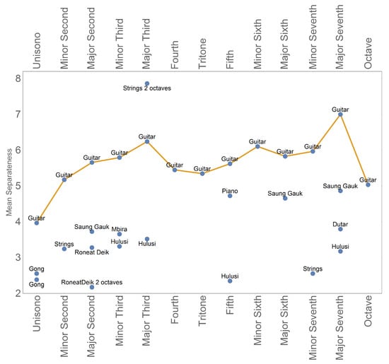
Figure 5.
Mean perception of separateness of all stimuli sorted according their musical interval (gongs are sorted as unisono). As the guitar tones form the familiar subgroup, and the guitar is the only instrument having all 13 intervals in the octave, they are connected with the yellow line. Except for the ’strings 2 octaves’ sound, which is the string pad sound, whose ISI histogram is shown in Figure 2, all non-familiar sounds are perceived as well separated, and therefore, as more fused compared to the familiar guitar sound. This points to a different perception strategy for familiar and unfamiliar sounds. Furthermore, the guitar sounds show the least separateness in unisono and octave as expected, and most separateness with the major seventh.
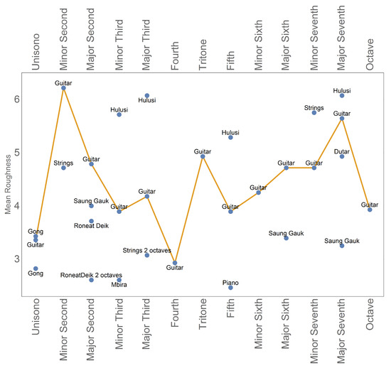
Figure 6.
Mean roughness perception of all stimuli; again, the guitar tones are connected with the yellow line. The roughness perception of the guitar sounds are as expected, least with unisono, octave, fourth, and fifth, and strongest with minor second, major seventh, and tritone. Still the non-familiar instruments are distributed above and below the guitar sounds, and do not show such a simple split as with separateness perception.
Using a one-way ANOVA, the significance p-value was found to be for separateness perception and for roughness when comparing the subjects’ judgement distributions of the 30 sound examples.
The separateness perception shows nearly all unfamiliar sounds being perceived as less separated than the guitar sounds. This points to different perception strategies between these two subsets: familiar and unfamiliar sounds. The only exception is the ’strings 2 octaves’ sound, which is shown with its ISI histogram in Figure 2’s middle plot. Here, the two notes are separated by over an octave and the ISI histogram shows two clearly distinguished peaks at the respective fundamental frequencies of the two notes in this sound sample.
When discussing instrument families the dutar and the saung gauk are both plucked stringed instruments like the guitar. Both are lower than the guitar tones in terms of separateness perception. This also holds for the two strings sounds, which are also supposed to be familiar to Western listeners and which are also perceived more fused than separated. These sounds are artificial string pad sounds, which have already been discussed above as unfamiliar, insofar as such synth sounds can be produced with arbitrary synthesis methods and parameters, which make these sounds unpredictable, and therefore, unfamiliar to listeners too. The only sound which is still familiar would then be the piano, which is indeed close to the guitar sound in terms of separateness. The least separated sounds are the gongs and the roneat deik, which are percussion instruments in the sense of having inharmonic overtone spectra, although the roneat deik is a pitched instrument. With the four instruments having a major seventh interval it is interesting to see how strong the influence of the instrument sound is in terms of separateness perception.
The roughness perception shown in Figure 6 does not show such a clear distinction between familiar and unfamiliar sounds. The guitar tones show a roughness perception as expected, least with the unisono, octave, fourth, and fifth, and strongest with the minor second, major seventh, and tritone. It is interesting to see that all four hulusi sounds are above the guitar, so perceived as more rough, following the roughness perception of the guitar qualitatively (major seventh most rough, fifth least rough, etc.). The mean and standard deviations for roughness and separateness perception are also displayed in Table 2 for the guitar sound and in Table 3 for the unfamiliar sounds.
Table 2.
Mean and standard deviations of roughness and separateness perception of the guitar tones.
Also, the gongs and the roneat deik are perceived with low roughness, they were also perceived as low in separateness. Still, overall, no perception strategy similar to that found for separateness can be found for roughness.
Comparing the perception of roughness and separateness in the guitar sounds, it appears that they are counteracting up to the fifth and aligning from the fifth to the octave qualitatively. So above the fifth it is likely for familiar sounds to be perceived separately when they are also perceived as rough. Below the fifth it is likely that these two perceptions are opposite. Therefore, the perception parameter of separateness is a different perception than that of roughness.
4.3. Correlation Between Perception and Simulation
In the section above, we found a clear split between familiar and unfamiliar sounds, pointing to two different perception strategies. Therefore, in this section, correlating perception to simulation, the two subgroups, familiar guitar sound and unfamiliar sounds, are correlated separately with simulation.
Figure 7 shows the Pearson’s correlation between simulation and separateness as well as roughness perception for the guitar and non-guitar sounds using entropy S. The upper graphs are roughness, the lower two separateness correlations, the left plots are the guitar and the right plots the non-guitar sounds, respectively. Each plot varies the standard deviation of the ISI histogram blurring in the range and a peak sharpness s in the range in 21 steps each (for details see above). Therefore, the left lower corner of each plot is the unprocessed ISI histogram, which might contain many peaks, most of them with low amplitude. With increasing a coincidence detection is performed, summing neighbouring peaks to a single peak. This reduces the number of peaks, but blurs them. When increasing s only sharp peaks are used. Of course, blurred peaks can only appear with higher values of . Therefore, higher values of s prevent large values of peaks being detected when they are so broad that they cannot reasonably have been built in a coincidence detection process as they are too far apart.
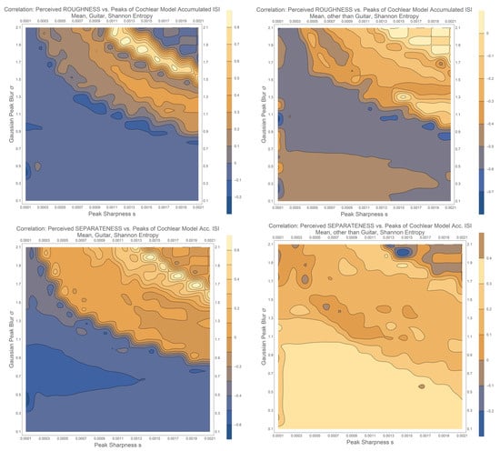
Figure 7.
Correlation between perceived roughness (upper plots) as well as separateness (lower plots) for the guitar tones (left plots) and all other non-guitar sounds (right plots) and the entropy S of the accumulated ISI spectrum, while post-processing the spectrum with Gaussian blurring with standard deviation and a peak sharpness s. All plots show a consistency or ridge from right/bottom to left/top as expected (see text for more detail). For roughness, the non-guitar sounds on the right have a negative correlation throughout, while the guitar sounds on the left have a positive correlation, pointing to an opposite perception between familiar and unfamiliar sounds. For separateness, the correlation between the guitar sounds on the left is positive at the right upper ridge and negative on the lower left side, while the non-guitar sounds on the left have a positive correlation on this lower left side and negative correlation at the upper right ridge, again showing opposite behaviour.
Examining the plots in Figure 7, concentrating on the left upper plot of roughness correlated with guitar tones, a ridge of positive correlation appears in the upper right corner. The rest of the plot is structured accordingly with a tendency of lower right to upper left ridges. Following the ridge with the highest correlation starting at on maximum s and ending at s = 0.0011 with maximum , the trade-off between and s leads to a reduction in the number of amplitudes down to only 3–5 amplitudes in the post-processed ISI histogram. This is a tremendous reduction taking into consideration that the number of amplitudes in the unprocessed lower left corner of the plots is between 700 and 800 amplitudes. On the right lower side of the ridge, with strong positive correlation, the peaks are not blurred to a maximum as the sharpness is very rigid, allowing only a few amplitudes. On the left upper side of the ridge the blurring is increased, still the sharpness criterion is eased, resulting in about the same number of amplitudes, 3–5. Indeed, in the upper right corner only one or even no amplitudes have survived.
Table 3.
Mean and standard deviations of roughness and separateness perception of the non-guitar tones.
Table 3.
Mean and standard deviations of roughness and separateness perception of the non-guitar tones.
| Sound | Interval | Roughness Mean | Roughness Std | Separateness Mean | Separateness Std |
|---|---|---|---|---|---|
| Mean | Std | Mean | Std | ||
| Saung Gauk | Major seventh | 3.25 | 1.80 | 4.86 | 2.53 |
| Saung Gauk | Major sixth | 3.39 | 1.87 | 4.66 | 2.27 |
| Saung Gauk | Major second | 4.00 | 2.64 | 3.72 | 2.31 |
| Dutar | Major seventh | 4.93 | 2.23 | 3.79 | 2.16 |
| Hulusi | Major third | 6.07 | 2.85 | 3.52 | 2.53 |
| Hulusi | Fifth | 5.29 | 3.00 | 2.345 | 1.82 |
| Hulusi | Minor third | 5.71 | 2.417 | 3.31 | 2.19 |
| Hulusi | Major seventh | 6.07 | 2.90 | 3.17 | 2.14 |
| Mbira | Minor third | 2.60 | 1.97 | 3.66 | 2.57 |
| Bama | Fundamental | 3.43 | 2.43 | 2.55 | 1.84 |
| Big Gong | ∼b2 | ||||
| Bama | Fundamental | 2.82 | 1.90 | 2.38 | 1.72 |
| Big Gong | ∼g#2 | ||||
| Roneat Deik | Major second | 3.71 | 2.27 | 3.28 | 2.31 |
| Roneat Deik | Two octaves | 2.61 | 2.04 | 2.17 | 2.16 |
| + major 2rd | |||||
| String Pad | Minor second | 4.71 | 2.48 | 3.24 | 2.23 |
| String Pad | Four octaves | 3.07 | 1.92 | 7.86 | 2.08 |
| + Major third | |||||
| Piano | Fifth | 2.46 | 1.69 | 4.72 | 2.23 |
| Strings | Minor seventh | 5.75 | 3.04 | 2.55 | 2.06 |
Now, comparing the two roughness plots for guitar (left upper) and non-guitar (right upper) sounds in Figure 7 they show opposite correlations. While the ridge in the guitar plot has a positive correlation, the correlation at the ridge position with the non-guitar tones is slightly negative; this plot shows negative correlations throughout. A similar behaviour holds for the separateness perception in the lower two plots of this figure. On the left, the guitar plot has a positive correlation at the ridge, while the non-guitar tones have a slightly negative correlation there, and are positive in the lower left part. Still, there is a difference between separateness and roughness. While the roughness plot is negative in the lower right corner of the plots for both guitar and non-guitar tones, the separateness plots show negative correlations with the guitar and positive ones with the non-guitar tones. In both cases, roughness and separateness, the ridge is positive with the guitar tones and slightly negative with the non-guitar sounds.
Finally, in Figure 8 the correlations of the standard deviations of the perceptual data with the ISI histogram entropy S are shown. They have some similarities with the plots of the mean of the perceptual parameters. Roughness for the guitar sounds again has a ridge at the upper right corner, still the lower right side of the plot is slightly positive, not negative like with the mean values. The roughness for the non-guitar sounds is all negative, like the mean case. For separateness, the guitar sounds have a negative ridge and a positive lower left corner, contrary to the mean values, this contrary behaviour is also seen with the non-guitar sounds compared to the mean case.
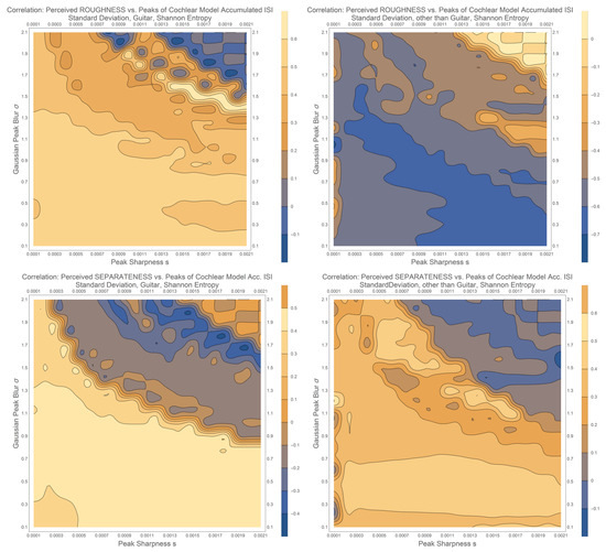
Figure 8.
Correlation of the standard deviation of the perceptual separateness and roughness with the ISI histogram entropy S. The correlation shows slight similarity with the mean value correlations of the perceptual dimensions.
The standard deviations and the number of peaks N and the amplitude-weighted peak sum W do not show considerable correlations. This points to the same direction as the correlations with the perceptual means, namely, that the entropy correlates better than the number of spikes N or W.
So, overall, a high standard deviation correlates positively with high entropy values in the lower left corner and negatively with a low entropy in the upper right corner. Therefore, we can conclude that when subjects were concentrating on strong coincidence detection, their judgements were much more consistent intersubjectively compared to the cases where subjects put their attention to low coincidence. The presence of only 3–5 amplitudes after strong coincidence detection points to subjects performing pitch perception, while low coincidence detection can be associated with timbre. Therefore, high correlations of perception with much coincidence, the ridges in the right upper corners of the plots, mean that subjects have put their attention to pitch. By contrast, a high correlation of perception with low coincidence detection, the left lower part of the plots, indicates subjects paying attention to timbre. This is expected as pitch is a much more consistent perception than timbre.
It is also interesting to have a look at the standard deviations for the perception of roughness and separateness, shown in Figure 9 and Figure 10, respectively. This perceptual standard deviation between subjects is expected to be low with familiar sounds, so subjects agree on their perception. It is expected to be higher with unfamiliar sounds, where subjects are not trained to these sounds and judge more individually.
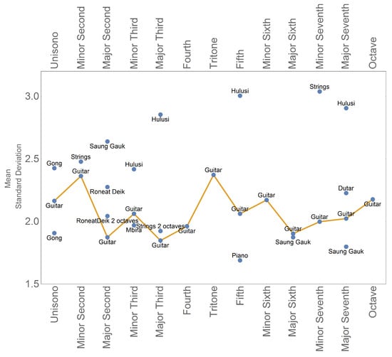
Figure 9.
Standard deviation for roughness perception. The guitar tones are among those sounds with the lowest standard deviation. Three hulusi and one strings sound have considerably larger SDs.
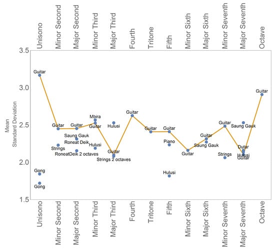
Figure 10.
Perceptual standard deviation of the separateness sounds. Here, the guitar tones are among those sounds with the highest SD. The gongs and one hulusi have considerably lower values.
Indeed, for roughness the guitar sounds have among the lowest values. Especially, the unfamiliar hulusi sounds are perceived considerably differently between subjects. Nevertheless, especially for the smaller tone intervals up to a minor third, the differences between familiar and unfamiliar sounds are less prominent.
For separateness, the standard deviations are highest for the guitar sounds, and subjects judged nearly all unfamiliar sounds more similarly. The two gongs are among the lowest values, indeed these sounds are special as one can decide to hear only one sound or many inharmonic partials.
Clearly, in terms of the judgements’ standard deviations a difference between roughness and separateness is present. This is also seen when examining the correlation between the mean and standard deviation of roughness perception, which is 0.62, pointing to increased uncertainty of judgements with higher values. While the correlation between mean and standard deviation for separateness is only 0.27, and so, seems to be more independent.
So, we conclude three points.
First, the familiar guitar sounds are perceived using only a small number of ISI histogram amplitudes, here 3–5, while the unfamiliar non-guitar tones are perceived using the broad range of many amplitudes in the ISI histogram. So the familiar sounds are perceived after intense coincidence detection, while the non-familiar sounds are perceived before coincidence detection, or only using a small part of it. For pitch detection, only a single spike is necessary for each period of f0. Timbre, on the contrary, needs more pitches to differentiate the sound. Therefore, a small number of spikes in the ISI point to pitch-based perception while many peaks allow for an elaborated timbre space. Also, the main peaks of the ISI histogram are associated with pitch in a harmonic sound as the main peaks correspond to a common periodicity, so to f0. Smaller amplitudes more strongly represent timbre, the elaboration of the sound. So, we can conclude that the perception strategy of familiar sounds uses pitch information and that of unfamiliar sounds uses timbre.
Second, separateness is correlated oppositely between familiar (negative correlation) and unfamiliar (positive correlation) sounds with low coincidence detection (lower right plot corners), while roughness is correlated negatively in both cases. This corresponds to the findings above, that separateness is perceived considerably more strongly with guitar tones than with non-guitar sounds, while roughness does not show this clear distinction. So, although for both it holds the pitch/timbre difference, separateness uses opposite strategies of perception while roughness uses the same correlation direction.
Third, judgements based on timbre are much more inconsistent than those based on pitch, which appears in the correlation between the standard deviation of the perceptual parameters and the entropy S of the ISI histograms.
These findings are based on the entropy calculated from the post-processed ISI histogram. Figure 11 shows the same correlations only taking the number N of surviving amplitudes into consideration. The results are similar in some respect, but show differences too. With the roughness guitar plot the ridge is again there, with a negative correlation in the right and left corners as before. Still, now the unfamiliar roughness case has a strong negative correlation when few amplitudes remain in the upper right corner and strong positive correlations in the many amplitude case in the lower left corner. Again, the perception is opposite, but much clearer than in the entropy case.
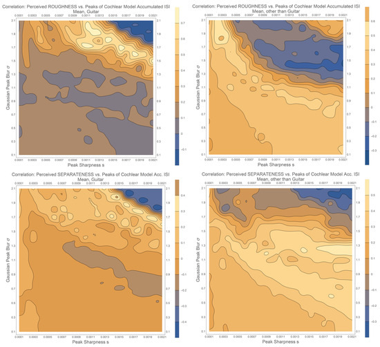
Figure 11.
Same as Figure 7 but correlation over number of ISI histogram amplitudes N. For roughness the non-guitar sounds on the right have a negative correlation in the upper right part and positive in the lower left, while the guitar sounds on the left have a positive correlation on the upper right ridge, again pointing to an opposite perception between familiar and unfamiliar sounds. For separateness, the correlation between the non-guitar sounds on the right is negative in the upper right part and positive in the lower left, while for the guitar sounds it is positive on the upper right ridge and slightly negative in the lower left part. Again, this is an opposite behaviour, although not as clear as with the entropy S in Figure 7.
For separateness the cases reverse too, the opposite correlation in the lower left corner disappears, and in the familiar and unfamiliar cases both regions correlate positively. Here, the ridge region changes correlation direction.
These findings contradict the findings from the perception test, namely, the clear split of familiar and unfamiliar sounds for separateness, pointing to an opposite perception strategy. Therefore, we conclude that using only amplitude counting is not perfectly in correspondence with the listening test, and therefore, more unlikely to be used by subjects to judge separateness.
Finally, the third method of weighted amplitudes W is shown in Figure 12. Here, the smallest correlations occur. Also, the clear structures which were found with entropy S and number of amplitudes N do not appear. Only the roughness guitar plot has some similarity with the ridge structure seen before. Therefore, we conclude that the amplitude-weighted ISI histogram does not correlate with perception.
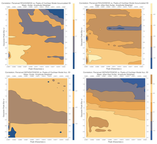
Figure 12.
Same as Figure 7 but correlation over amplitude-weighted ISI histogram W. The plots are considerably different from the entropy S, Figure 7, and number of different amplitudes N in Figure 11. Although the guitar roughness plot (top left) shows a kind of ridge as seen before, the correlations are very small. The roughness non-guitar plot (top right) has large negative correlations at a line at . The separateness guitar plot again has low correlations, while the non-guitar separateness plot has larger positive correlations in its lower part, slightly similar to the roughness non-guitar plot. Still, it seems that amplitude weighting does not reasonably correlate with perception.
5. Conclusions
The results point to two different perception strategies when listeners are asked to judge separateness and roughness of familiar and unfamiliar sounds. With familiar sounds a strong coincidence detection seems to take place, where listeners concentrate on only a small number of spikes representing merely pitch. With unfamiliar sounds they use the raw input much more strongly, without the coincidence detection reduction, so on a more elaborated pitch, on timbre. This corresponds to the overall experience listeners reported for the unfamiliar sounds, namely, that they could often not tell if the sounds consisted of two pitches or only one, or could not clearly identify one of the pitches. Therefore, they needed to rely on timbre rather than on extracted pitches.
A second perception strategy seems to happen when listeners are asked to judge separateness or roughness of sounds. With roughness, timbre is the part listeners concentrate on; with separateness perception the strategy changed between familiar and unfamiliar sounds. With unfamiliar sounds separateness is correlated positively with a complex sound; with familiar sounds timbre is correlated negatively. So in unfamiliar multi-pitch sounds the pitches are perceived separately when the timbre is complex, while with familiar sounds the pitches are found separately when the timbre is simpler. It might be that listeners find it easier to separate pitches with familiar sounds when the timbre is simpler. Still, if they are not familiar with the sound and not able to extract pitches anyway, they find complex spectra more separate than fused.
In all cases, judgements based on timbre are much more inconsistent between subjects than those based on pitch.
In terms of neural correlates of roughness and separateness perception, the entropy of the ISI histogram is much better able to explain perception compared to the number of different amplitudes or, even worse, the weighted amplitude sum. This is expected, as entropy is a more complex way of summing a sensation into a single judgement or separateness or roughness than the other methods, as entropy gives an estimation of the distribution of amplitudes in the spectrum, and therefore, their relation. Other methods might even be better suited, which is beyond the scope of the present paper to discuss.
Overall, it appears that many judgements of subjects are based on low-level parts of the auditory pathway, before extended coincidence detection. This points to the necessity of perceiving timbre and pitch as a field of neural activity.
Funding
This research received no external funding.
Institutional Review Board Statement
Not applicable.
Informed Consent Statement
Not applicable.
Data Availability Statement
The raw data supporting the conclusions of this article will be made available by the authors on request.
Conflicts of Interest
The authors declare no conflicts of interest.
References
- Schneider, A. Pitch and Pitch Perception. In Springer Handbook of Systematic Musicology; Springer: Berlin/Heidelberg, Germany, 2018; pp. 605–685. [Google Scholar]
- von Helmholtz, H. Die Lehre von den Tonempfindungen als Physiologische Grundlage für die Theorie der Musik [On the Sensations of Tone As a Physiological Basis for the Theory of Music]; Vieweg, Braunschweig: Decatur, IL, USA, 1863. [Google Scholar]
- Schneider, A. Perception of Timbre and Sound Color. In Springer Handbook of Systematic Musicology; Springer: Berlin/Heidelberg, Germany, 2018; pp. 687–725. [Google Scholar]
- Bregman, A.S. Auditory Scene Analysis: The Perceptual Organization of Sound; MIT Press: Cambridge, MA, USA, 1994. [Google Scholar]
- Benetos, E.; Dixon, S. Multiple-instrument polyphonic music transcription using a temporally constrained shift-invariant model. J. Acoust. Soc. Am. 2013, 133, 1727–1741. [Google Scholar] [CrossRef] [PubMed]
- Jansson, A.; Bittner, R.M.; Ewert, S.; Weyde, T. Joint singing voice separation and f0 estimation with deep u-net architectures. In Proceedings of the 2019 27th European Signal Processing Conference (EUSIPCO), Coruña, Spain, 2–6 September 2019; pp. 1–5. [Google Scholar]
- McLeod, A.; Schramm, R.; Steedman, M.; Benetos, E. Automatic transcription of polyphonic vocal music. Appl. Sci. 2017, 7, 1285. [Google Scholar] [CrossRef]
- Schramm, R. Automatic Transcription of Polyphonic Vocal Music. In Handbook of Artificial Intelligence for Music. Foundations, Advanced Approaches and Developments for Creativity; Springer: Berlin/Heidelberg, Germany, 2021; pp. 715–736. [Google Scholar]
- Lin, K.W.E.; Balamurali, B.T.; Koh, E.; Lui, S.; Herremans, D. Singing voice separation using a deep convolutional neural network trained by ideal binary mask and cross entropy. Neural Comput. Appl. 2018, 32, 1037–1050. [Google Scholar] [CrossRef]
- Dessein, A.; Cont, A.; Lemaitre, G. Real-time polyphonic music transcription with non-negative matrix factorization and beta-divergence. In Proceedings of the ISMIR—11th International Society for Music Information Retrieval Conference, Utrecht, The Netherlands, 9–13 August 2010; pp. 489–494. [Google Scholar]
- Matsunaga, T.; Saito, H. Multi-Layer Combined Frequency and Periodicity Representations for Multi-Pitch Estimation of Multi-Instrument Music. IEEE/ACM Trans. Audio Sep. 2024, 99, 3171–3184. [Google Scholar] [CrossRef]
- Vincent, E.; Bertin, N.; Badeau, R. Adaptive harmonic spectral decomposition for multiple pitch estimation. IEEE/ACM Trans. Audio, Speech, Lang. Process. 2010, 18, 528–537. [Google Scholar] [CrossRef]
- Grey, J.M.; Moorer, J.A. Perceptual evaluations of synthesized musical instrument tones. J. Acoust. Soc. Am. 1977, 62, 454–462. [Google Scholar] [CrossRef]
- Iverson, P.; Krumhansl, C.L. Isolating the dynamic attributes of musical timbre. J. Acoustic. Soc. Am. 1993, 94, 2595–2603. [Google Scholar] [CrossRef] [PubMed]
- McAdams, S.; Winsberg, S.; Donnadieu, S.; De Soete, G.; Krimphoff, J. Perceptual scaling of synthesized musical timbres: Common dimensions, specifities, and latent subject classes. Psychol. Rev. 1995, 58, 177–192. [Google Scholar]
- Bader, R. Nonlinearities and Synchronization in Musical Acoustics and Music Psychology; Current Research in Systematic Musicology; Springer: Berlin/Heidelberg, Germany, 2013; Volume 2. [Google Scholar]
- Ziemer, T.; Schultheis, H. PAMPAS: A Psycho-Acoustical Method for the Perceptual Analysis of multidimensional Sonification. Front. Neurosci. 2022, 16, 930944. [Google Scholar] [CrossRef]
- Bader, R. Pitch and timbre discrimination at wave-to-spike transition in the cochlea. arXiv 2017, arXiv:1711.05596. [Google Scholar] [CrossRef]
- Haken, H. Brain Dynamics, Springer Series in Synergetics, 2nd ed.; Springer: Berlin/Heidelberg, Germany, 2008. [Google Scholar]
- Baars, B.J.; Franklin, S.; Ramsoy, T.Z. Global workspace dynamics: Cortical binding and propagation enables conscious contents. Front Psychol. 2013, 4, 200. [Google Scholar] [CrossRef] [PubMed]
- Fries, P.; Neuenschwander, S.; Engel, A.K.; Goebel, R.; Singer, W. Rapid feature selective neuronal synchronization through correlated latency shifting. Nat. Neurosci. 2001, 4, 194–200. [Google Scholar] [CrossRef] [PubMed]
- Buhusi, C.V.; Meck, W.H. What makes us tick? Functional and neural mechanisms of interval timing. Nat. Rev. Neurosci. 2005, 6, 755–765. [Google Scholar] [CrossRef] [PubMed]
- Hartmann, L. Neuronal synchronization of musical large-scale form: An EEG-study. Proc. Mtgs. Acoust. 2014, 22, 035001. [Google Scholar] [CrossRef]
- Barrie, J.M.; Freeman, W.J.; Lenhart, M.D. Spatiotemporal analysis of prepyriform, visual, auditory, and somesthetic surface EEGs in trained rabbits. J. Neurophysiol. 1996, 76, 520–539. [Google Scholar] [CrossRef] [PubMed]
- Kozma, R.; Freeman, W.J. (Eds.) Cognitive Phase Transitions in the Cerebral Cortex—Enhancing the Neuron Doctrine by Modeling Neural Fields; Springer Series Studies, System, Decision, and Control; Springer: Berlin/Heidelberg, Germany, 2016. [Google Scholar]
- Ohl, F.W. On the Creation of Meaning in the Brain—Cortical Neurodynamics During Category Learning. In Cognitive Phase Transitions in the Cerebral Cortex—Enhancing the Neuron Doctrine by Modeling Neural Fields; Springer Series Studies, System, Decision, and Control; Kozma, R., Freeman, W.J., Eds.; Springer: Berlin/Heidelberg, Germany, 2016; pp. 147–159. [Google Scholar]
- Bader, R. Cochlea spike synchronization and coincidence detection model. Chaos 2018, 023105, 1–10. [Google Scholar]
- Joris, X.; Lu, H.-W.; Franken, T.; Smith, H. What, if anything, is coincidence detection? J. Acoust. Soc. Am. 2023, 154, A242. [Google Scholar] [CrossRef]
- Joris, P.X.; Carney, L.H.; Smith, P.H.; Yin, T.C.T. Enhancement of neural synchronization in the anteroventral cochlea nucleus. I. Responses to tones at the characteristic frequency. J. Neurophysiol. 1994, 71, 1022–1036. [Google Scholar] [CrossRef] [PubMed]
- Joris, P.X.; Carney, L.H.; Smith, P.H.; Yin, T.C.T. Enhancement of neural synchronization in the anteroventral cochlea nucleus. II. Responses in the tuning curve tail. J. Neurophysiol. 1994, 71, 1037–1051. [Google Scholar] [CrossRef]
- Kreeger, L.J.; Honnuraiah, S.; Maeker, S.; Goodrich, L.V. An anatomical and physiological basis for coincidence detection across time scales in the auditory system. bioRxiv 2024. [Google Scholar] [CrossRef]
- Stoll, A.; Maier, A.; Krauss, P.; Schilling, A. Coincidence detection and integration behavior in spiking neural networks. Cogn. Neurodyn. 2023, 1–13. [Google Scholar] [CrossRef]
- Schonfield, B.R. Central Decending Auditory Pathways. In Auditory and Vestibular Efferents; Ryugo, D.K., Fay, R.R., Popper, A.N., Eds.; Springer: Berlin/Heidelberg, Germany, 2011; pp. 261–290. [Google Scholar]
- Buzsáki, G. Rhythms of the Brain; Oxford University Press: Oxford, UK, 2006. [Google Scholar]
- Ferrante, M.; Ciferri, M.; Toschi, N. R&B—Rhythm and Brain: Cross-subject Decoding of Music from Human Brain Activity. arXiv 2024, arXiv:2406.15537v1. [Google Scholar]
- Thaut, M. Rhythm, Music, and the Brain: Scientific Foundations and Clinical Applications; Routledge: London, UK, 2007. [Google Scholar]
- Dau, T.; Püschel, D.; Kohlrausch, A. A quantitative model of the “effective” signal processing in the auditory system. I. Model structure. J. Acoust. Soc. Am. 1996, 99, 3615–3622. [Google Scholar] [CrossRef] [PubMed]
- Dau, T.; Püschel, D.; Kohlrausch, A. A quantitative model of the “effective” signal processing in the auditory system. II. Simulations and measurements. J. Acoust. Soc. Am. 1996, 99, 3623–3631. [Google Scholar] [CrossRef] [PubMed]
- Lewicki, M.S. Efficient coding of natural sounds. Nat. Neurosci. 2002, 5, 356–363. [Google Scholar] [CrossRef] [PubMed]
- Cariani, P. Temporal Codes, Timing Nets, and Music Perception. J. New Music. Res. 2001, 30, 107–135. [Google Scholar] [CrossRef]
- Cariani, P. Temporal Coding of Periodicity Pitch in the Auditory System: An Overview. Neural Plast. 1999, 6, 147–172. [Google Scholar] [CrossRef] [PubMed]
- Goldstein, J.L.; Gersen, A.; Srulovicz, P.; Furst, M. Verification of the Optimal Probabilistic Basis of Aural Processing of Pitch of Complex Tones. J. Acoust. Soc. Am. 1978, 63, 486–497. [Google Scholar] [CrossRef] [PubMed]
- Bader, R. How Music Works—A Physical Culture Theory; Springer: Berlin/Heidelberg, Germany, 2021. [Google Scholar]
- Sawicki, J.; Hartmann, L.; Bader, R.; Schöll, E. Modelling the perception of music in brain network dynamics. Front. Netw. Physiol. 2020, 2, 910920. [Google Scholar] [CrossRef]
- Bader, R. Modeling Temporal Lobe Epilepsy during Music Large-Scale Form Perception Using the Impulse Pattern Formulation (IPF) Brain Model. Electronics 2024, 13, 362. [Google Scholar] [CrossRef]
- Linke, S.; Bader, R.; Mores, R. Modeling synchronization in human musical rhythms using Impulse Pattern Formulation (IPF). arXiv 2021, arXiv:2112.03218. [Google Scholar]
- Rossing, T. Science of Percussion Instruments; World Scientific: Singapore, 2001. [Google Scholar]
Disclaimer/Publisher’s Note: The statements, opinions and data contained in all publications are solely those of the individual author(s) and contributor(s) and not of MDPI and/or the editor(s). MDPI and/or the editor(s) disclaim responsibility for any injury to people or property resulting from any ideas, methods, instructions or products referred to in the content. |
© 2024 by the author. Licensee MDPI, Basel, Switzerland. This article is an open access article distributed under the terms and conditions of the Creative Commons Attribution (CC BY) license (https://creativecommons.org/licenses/by/4.0/).