Ray Tracing of the New Multi-Modal X-ray Imaging Beamline PolyX at SOLARIS National Synchrotron Radiation Centre

Abstract

The aim of the presented research is to evaluate the potential performance of a new bending magnet X-ray beamline—PolyX, designed for microimaging and microspectroscopy at the National Synchrotron Radiation Centre SOLARIS in Krakow. Due to the short beamline length (<15 m), PolyX uses compact polycapillary and single-bounce monocapillary optics for X-ray focusing in the 4–15 keV energy range. Polycapillary optics require a dedicated approach for an efficient simulation of X-ray propagation in multiple capillary channels. Therefore, the PolyX beamline was ray traced by combining XRT (XRayTracer) and polycap libraries. In addition, to estimate the X-ray fluorescence spectra excited by focused beams, Monte Carlo simulations were conducted using XMI-MSIM. All simulations were aimed to estimate the crucial X-ray beam properties, i.e., the flux, the spot size, and the energy spectrum, for monochromatic and polychromatic X-ray beams.

1. Introduction

SOLARIS is a synchrotron radiation facility with a 1.5 GeV storage ring located in Krakow, southern Poland. It was commissioned in 2015, and it is a third-generation source of soft X-rays with a critical photon energy of 2 keV. Currently, there are five active beamlines and three under construction/commissioned [1]. One of them is PolyX [2]—a simple and compact beamline that aims to provide both unfocused and focused beams from the bending magnet for X-ray microimaging and X-ray microspectroscopy experiments. The main techniques available with PolyX are μ-XRF, μ-XAS, μ-CT with absorption and phase contrast as well as plenoptic X-ray imaging [3]. The beam focusing is achieved using polycapillary optics. Those very compact devices use the effect of total external reflection of X-rays inside thousands of small bent hollow glass tubes. PolyX will take advantage of the very high acceptance of polycapillary lenses, allowing for it to achieve highly intense white, pink, or monochromatic 4–15 keV X-rays focused down to 10 μm. For better focusing (down to 2 μm), an ellipsoidal single-bounce monocapillary lens will be used.

In the field of X-ray physics, ray tracing refers to the simulation of X-ray beams propagating through different materials and optical components. Ray-tracing simulations have become an essential tool in X-ray physics for designing and optimizing synchrotron beamlines [4,5,6,7] and optical elements, including single-bounce capillary devices [8,9,10] as well as polycapillary optics [11,12,13]. Ray-tracing simulations allow for the evaluation of X-ray beam properties such as flux, spot size, and energy spectrum, which are crucial for optimizing the performance of a beamline. Moreover, by simulating the entire beamline, it is possible to identify and correct potential issues before the actual installation of the beamline, as well as to predict the performance of the beamline.

The goal of this research is to use ray tracing to predict the performance of the PolyX beamline, specifically the photon flux on the sample (in both polychromatic and monochromatic modes) and the achievable beam size with different available polycapillary lenses, as well as single-bounce ellipsoidal monocapillary. Furthermore, the ray-tracing model will enable the simulation of the beam characteristics in all possible configurations of the adjustable beamline components, such as filters and slits.

In this paper, for PolyX beamline ray tracing, we used the XRT toolkit [5]. XRT is a Python-based software library for beamline simulation and analysis in X-ray regimes. It provides the classes for many beamline elements, the propagation engine in ray and wave approximations with full account for shapes and material properties, and high-quality visualization capabilities. While XRT enables the user to simulate X-ray propagation inside polycapillary optics, such calculations are very time-consuming. Therefore, we used XRT (for simulation of standard beamline components) in conjunction with the polycap library [7]. Polycap is a multithreaded Monte Carlo-based X-ray ray tracing code dedicated to the simulation of polycapillary optics. Moreover, to evaluate the performance of the beamline in fast, high-resolution μ-XRF mapping, additional simulations of X-ray spectra with the XMI-MSIM [14] tool were performed.

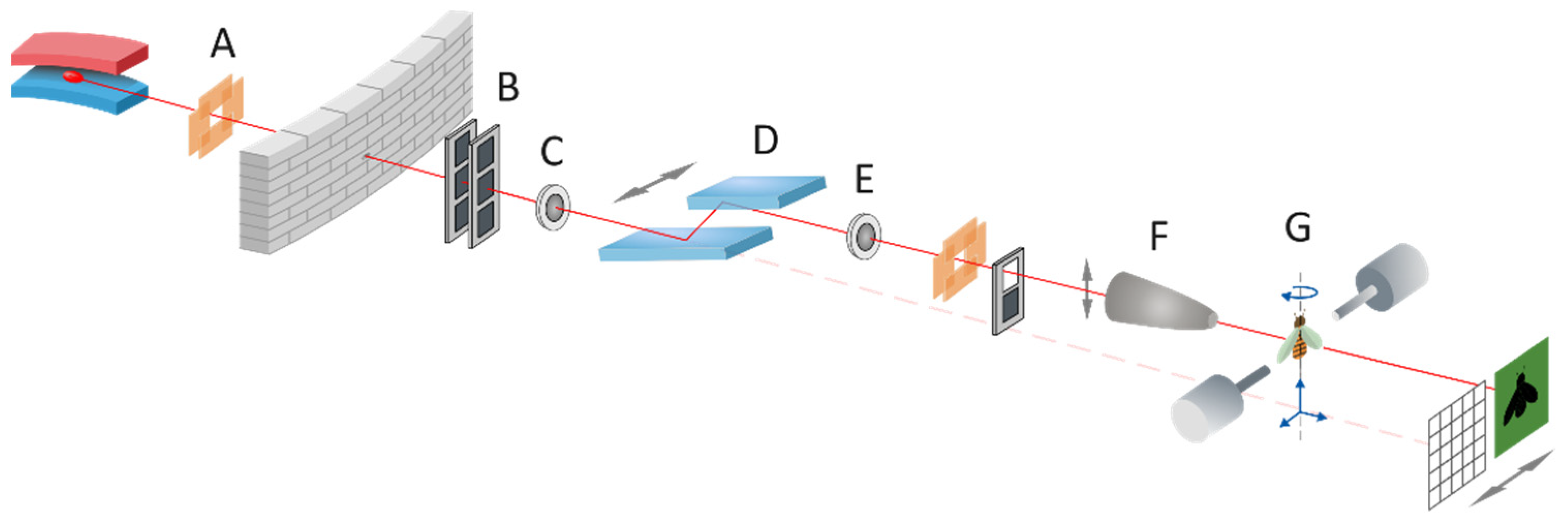
2. Beamline Description

The source of the PolyX beamline is a 1.31 T bending magnet from the SOLARIS storage ring. The detailed information about the source is given in

Table 1. Bending magnet (X-ray source) parameters used in simulations.

Parameter	Value
Electron beam energy	1.5 GeV
Maximum current	500 mA
Electron beam sizes (σx, σz)	44 μm, 30 μm
Electron beam emittance (εx, εz)	8.05 nm·rad, 0.065 nm·rad
BM magnetic field	1.31 T

and the scheme of the beamline is provided in Figure 1. The beamline optics are designed to deliver either a polychromatic white beam or a monochromatized beam to the end station. Two types of interchangeable monochromators are planned: a double crystal monochromator (DCM) and a double multilayer monochromator (DMM). The list of all main components of the beamline with corresponding distances from the bending magnet is shown in

Table 2. Positions of simulated beamline components.

	Component	Distance from the Source [mm]
1	Fixed mask 1	2314
2	White beam slits	5122.5
3	Fixed mask 2	6704
4	White beam filters	8790
5	Be window 1 (250 µm)	9110
6	Monochromator	11,570
7	Be window 2 (500 µm)	12,625
8	Capillary optics	~14,450 (depending on the optic in use)
9	Sample	14,500

.

A DCM uses two crystals made of Si(111) that are precisely aligned to diffract X-rays of a specific wavelength with a bandwidth of ~ 1.4 × 10⁻⁴ and a constant vertical offset of 10 mm. The dimensions (width × length) of the first and the second crystal are 35 mm × 55.5 mm and 35 mm × 140 mm, respectively. A DMM uses a pair of multilayer mirrors to diffract and reflect X-rays to achieve monochromatization with a bandwidth of several percent. Each mirror has two different stripes of multilayer structures next to each other. The first stripe was prepared to work with the energy range of 4–8 keV. It has a Ni/B₄C multilayer coating with 75 periods, a period of 4 nm and a metal layer thickness-to-period ratio of 0.4. The second stripe is dedicated to work in the 7.5–15 keV energy range. It has a Mo/B₄C multilayer coating with 115 periods, a period of 2.6 nm and a metal layer thickness-to-period ratio of 0.4. The dimensions of both stripes were set to 20 mm × 280 for the stripes on the first optics, and to 20 × 172 mm for the stripes on the second optics. The vertical offset between the second and the first crystal is again set to the fixed value of 10 mm.

In order to achieve the focused beam on the sample, two types of capillary optics will be used at PolyX. Seven different polycapillary lenses (from Helmut–Fisher formerly IfG, Germany and XOS, USA) will be interchangeably used to achieve a focal spot in range from 10 to 100 µm. A narrower beam will be achieved with an achromatic ellipsoidal single-bounce monocapillary lens (AEXML) with a 30 nm Pt coating from Sigray, USA. The details of the selected optical elements are given in

Table 3. Parameters of simulated optics.

Alias	Working Distance [mm]	Optics Length [mm]	Optics Upstream Diameter [mm]	Optics Downstream Diameter [mm]	Upstream Capillary Channel Diameter [um]	No. of Capillaries
poly f = 2.5	2.5	37	4.2	0.83	0.75	313,136
poly f = 14.5	14.5	63.75	6.4	2	3.3	97,801
poly f = 40	40	41	6.5	4.5	7.5	101,144
AEXML	20.5	50	1	0.54	-	1

(the remaining polycapillaries are described in the supplementary materials).

The main measurement modes that will be routinely used at PolyX are elemental microimaging by µ-XRF, elemental speciation by µ-XAS and absorption/phase-contrast imaging by µ-CT. Other techniques that are planned to be available at the beamline are confocal-XRF for 3D elemental imaging, high-resolution plenoptic X-ray imaging and µ-XRD for crystalline phase speciation. Several different X-ray detectors will be installed at the end station. The first group—spectrometry detectors—is composed of two silicon drift detectors (SDD) with 80 mm² active area (one with 25 µm Be window and one with ML3.3 Extreme window) by Hitachi High-Tech. As a digital pulse processor, a DANTE system from XGLab will be used. The detectors will work in the back-scatter geometry (at 45° with the sample perpendicular to the beam); however, the standard 45°/45° geometry will be also achievable. The ultra-thin ML3.3 window was chosen to allow the detection of low-energy X-rays in a helium atmosphere. The second class of detectors are those devoted to imaging: hybrid pixel EIGER 2S 1 M with 77.1 × 79.7 mm² active area (75 × 75 µm² pixel size) by Dectris and white beam microscope by OptiquePeter with variable scintillators and Edge 5.5 sCMOS camera (2560 × 2160 pixel) by PCO. The third class of detectors will be beam monitors: ionisation chambers by FMB Oxford and PIN Diodes by Hamamatsu. The key design aspect of the experimental station is to allow multi modal experiments as well as easy switching between different modes.

3. Methods

In this work, we used a Python-based library XRT [5] to perform ray-tracing simulations of the standard beamline components. The simulations covered all crucial components of the beamline, including the bending magnet source characterised by parameters from Table 1. Other elements simulated by XRT are slits and masks, beryllium windows, filters, a double crystal monochromator (DCM) or a double multilayer monochromator (DMM), as well as anellipsoidal single-bounce monocapillary lens (AEXML). Additionally, the polycap library [7] combined with XRT library was used to perform efficient ray tracing of the beamline with the polycapillary lenses.

The simulation took into account the expected distances from the source for every element, as listed in Table 2. For all simulations of DCM, the beam was slit down vertically to keep the bandwidth dE/E = 0.02%.

The combination of XRT and polycap libraries enabled an efficient modeling of the whole beamline. The XRT was used to obtain the rays at the entrance surface of polycapillary, and polycap ray-traced X-ray propagation inside polycapillary device. Importantly, the parameters (position, direction, polarization) of each ray were directly transferred from xrt to polycap by in-house developed write/read Python functions.

The simulations of polycapillary optics were performed with the assumption that all of them had ellipsoidal shapes. The parameters of simulated lenses are presented in Table 2. The naming of polycapillary lenses (aliases) was based on their working distances. For AEXML optics, the distortion from perfect shape was implemented as a slope error of 10 µrad (RMS), in order to estimate a realistic spot size. In Figure 2, Figure 3 and Figure 4, the examples of ray visualizations are presented, just upstream of the entrance to polycapillary and monocapillary lenses as well as in their focal planes. The left panels of Figure 2 and Figure 3 (created with the XRT library visualisation tool) show spatial distributions of the simulated rays together with their projections on vertical and horizontal axes. The right panels show energy distributions. The position and energy mean values with FWHM values are also given. N_all and N_good are values of all simulated rays and rays reflected within the working optical surfaces, respectively. The total photon flux (Φ) is also given.

The simulations of X-ray spectra were carried out with the XMI-MSIM tool. The number of photons per interval and discrete line were set to 10,000 and 100,000, respectively. The single interaction per photon trajectory was simulated, and Poisson noise was generated. The default detector response was used.

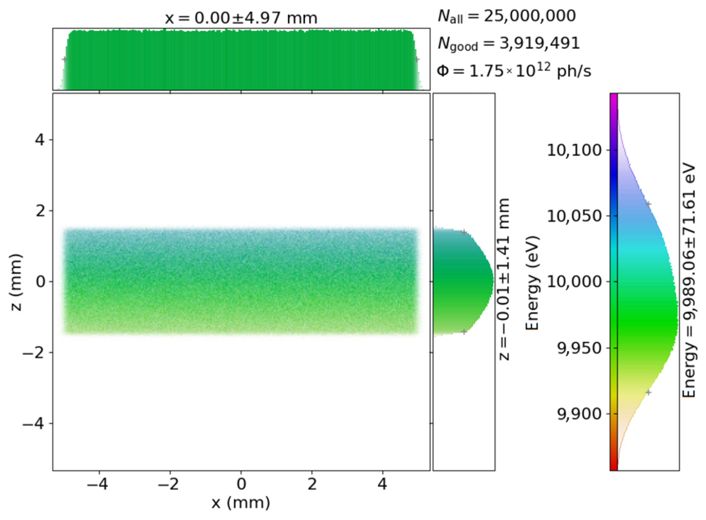
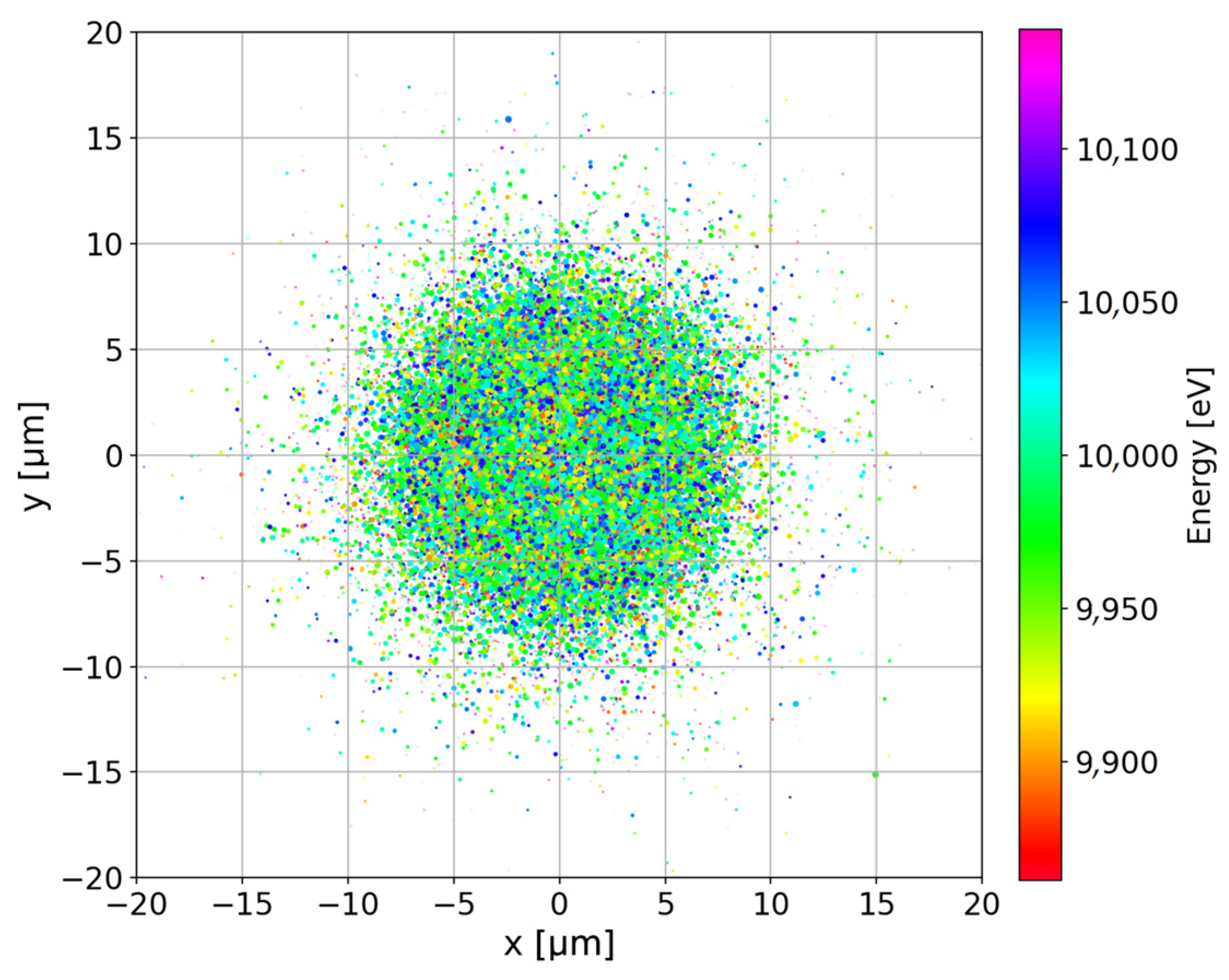
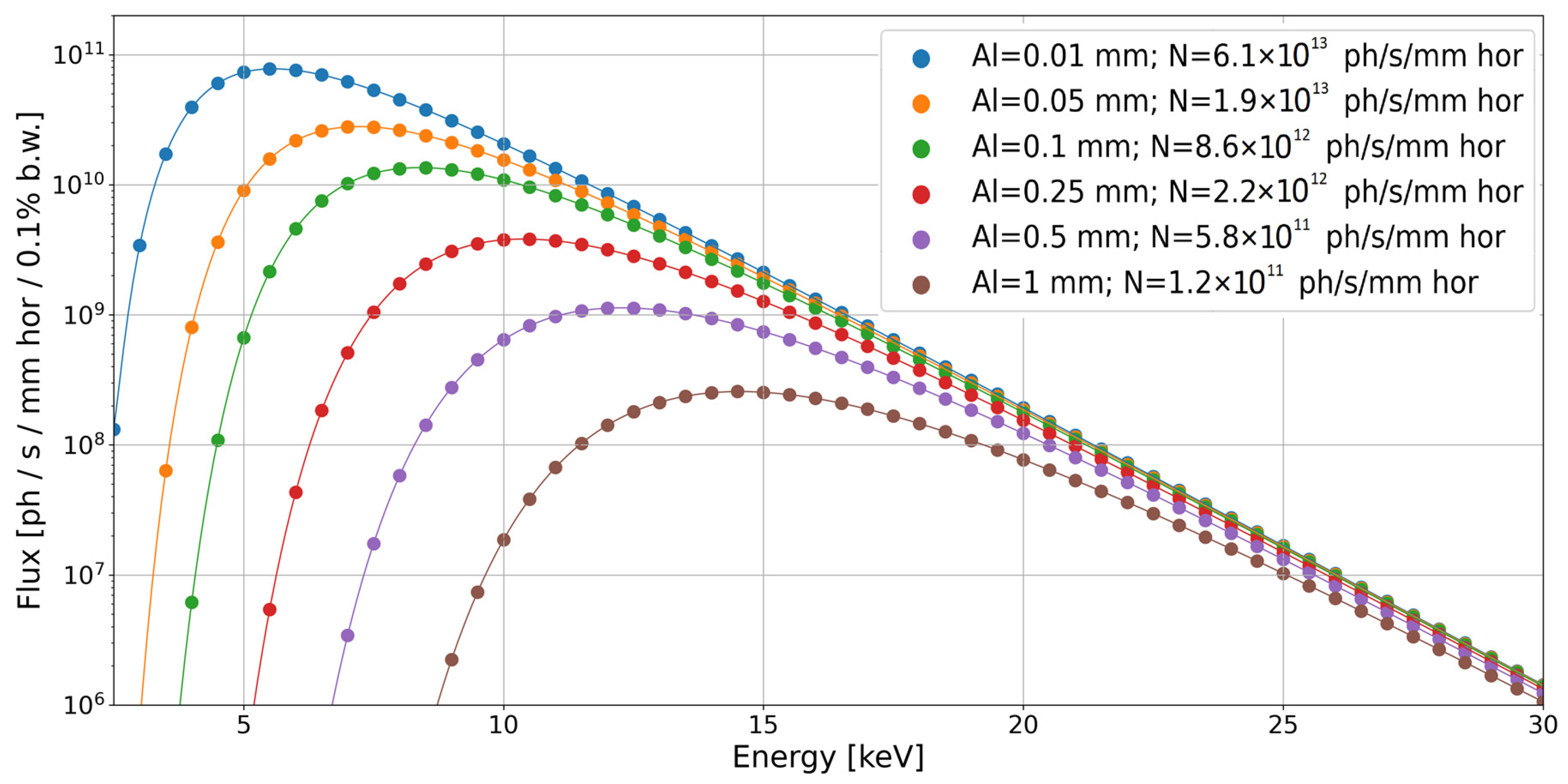
4. Results and Discussion

Our simulations were performed using a range of configurations for the beamline components and X-ray focusing optics. The results of the simulations were used to evaluate the X-ray beam properties, including the flux, the spot size, and energy resolution for different configurations.

First, we performed simulations of the beamline for the white beam mode, i.e., without any monochromator. To shape the X-ray spectrum, Al filters of variable thickness (0.01 mm, 0.05 mm, 0.1 mm, 0.25 mm, 0.5 mm, 1 mm) were simulated. White beam energy spectra and the total flux (denoted as N in the legend) were simulated for full vertical beam size and for 1 mrad horizontal slit opening (Figure 5).

Next, we calculated the flux for both monochromator types, DCM and DMM. For DMM, both stripes were simulated for the relevant energy ranges. The results are shown in Figure 6.

Subsequently, we focused on the prediction of achievable beam parameters, while using different capillary optics. For the sake of clarity, the next figures show results for only three types of polycapillary lenses and for one monocapillary lens. However, the supplementary materials present selected results for the other four available polycapillary lenses.

The transmission efficiencies of the focusing elements (Figure 7) were calculated by performing the following steps: (i) slits were set to be fully opened in the vertical and horizontal directions, (ii) a simulation for the white beam was conducted (without any Al filters) for different energies, in the range of 4–15 keV, the step between the points was 0.5 keV, and bandwidth for every step was 0.1%, (iii) the flux N₀ was calculated for rays that were accepted into the optics entrance, (iv) the flux N was calculated in the focal spots, and (v) the transmission was calculated as T = N/N₀.

The transmission efficiency for AEXML is significantly higher than for polycapillary optics since, in contrast to polycapillary optics, it relies on single-bounce transmission. AEXML optic has two distinguishable drops, which are caused by the L absorption edges of the platinum inner coating.

The spot sizes in the focal planes (Figure 8 and Figure 9) were estimated using the same white beam simulations as described above for transmission efficiencies. First, vertical and horizontal histograms of the rays were calculated, then histograms of FWHMs were determined for both axes and the average value was taken as the final spot size.

For polycapillary lenses and for an ellipsoidal single-bounce monocapillary lens, the full energy spectra for the beams that passed through the optics were estimated during the simulations. These results were used to calculate the achievable fluxes in the focal spot. For the white beam mode, the different thicknesses of Al filters were used in simulations (Figure 10). The flux was also estimated for the beam that passed through one of the monochromators (DCM or DMM described in the previous section) and later focused by the lenses (Figure 11). The results for a subset of simulated lenses are presented in supplementary materials.

To predict the results of µ-XRF experiments, simulations of the X-ray fluorescence spectra from two different samples were performed with XMI-MSIM. Simulations were performed for the beam focused with AEXML, as a worst-case scenario in terms of expected beam intensity and the best scenario in terms of spatial resolution. All the simulations were carried out for a silicon drift detector equipped with ML3.3 Extreme window, helium atmosphere and backscatter geometry (90° angle between the beam and the sample plane and 45° angle between the sample plane and the detector axis) with a sample-detector distance of 3 cm and an acquisition time of 1 s. Two excitation modes were chosen: monochromatic (5 keV, 10 keV and 15 keV) with DMM and polychromatic with the white beam filtered with various aluminium filters. The sample of biological thin tissue section (4 µm), one of the most demanding materials, was chosen. The elemental composition of the tissue was selected based on the literature data [15] and is given in

Table 4. Elemental composition and intensities of Kα lines (in counts per second) for simulated thin tissue sample.

		Weight Fraction		DMM			White Beam Filtered with Al
Z	Elem.	Value	Unit	5 keV	10 keV	15 keV	0.5 mm	1 mm	2 mm
1	H	8.1	%
6	C	64.8	%
7	N	9.8	%
8	O	13.7	%
11	Na	0.2	%	1600	23	<1	380	47	4
12	Mg	620	µg/g	530	17	<1	290	35	3
15	P	1.2	%	110k	1800	45	30k	3800	310
16	S	0.8	%	110k	1800	46	30k	3800	320
17	Cl	0.3	%	58k	1000	26	16k	2100	180
19	K	1.0	%	380k	6900	180	120k	15k	1300
20	Ca	130	µg/g	6800	120	3	2100	270	22
25	Mn	10	µg/g	-	29	<1	510	66	6
26	Fe	210	µg/g	-	770	21	13k	1700	150
29	Cu	120	µg/g	-	710	21	11k	1600	150
30	Zn	180	µg/g	-	1200	36	18k	2800	250
34	Se	2	µg/g	-	-	<1ss	110	32	4
35	Br	3	µg/g	-	-	<1	120	65	6
37	Rb	35	µg/g	-	-	-	700	310	67
38	Sr	95	µg/g	-	-	-	1200	600	160

, together with the simulated elemental intensities. The simulated spectra for both excitation modes are shown in Figure 12 and Figure 13. As can be seen for 5 keV, 10 keV, and white beam filtered with 1 mm Al, the expected count rates of the elements up to zinc are high enough to make fast XRF imaging feasible even with the acquisition times being much lower than 1 s. Heavier and low-abundant elements like Se, Br, Rb and Sr can be efficiently excited with only the polychromatic beam; however, the detection of those elements will be very difficult due to the poor signal-to-noise ratio.

In order to acquire information about the capabilities of analysis of higher Z elements with the high-energy tail of the polychromatic excitation spectrum, a 1mm-thick soda-lime glass (72% SiO₂, 14% Na₂O, 12% CaO, 2% Al₂O₃) sample doped with some elements (Se, Sr, Zr, Mo, W, Pb, Th, U) at 100 µg/g level was used. The results of the simulations for 1 mm, 2 mm and 4 mm aluminium filters are shown in

Table 5. Elemental XRF intensities (in counts per second) for simulated glass sample.

	Elem.	Line	Weight Fraction [µg/g]	1 mm Al	2 mm Al	4 mm Al
34	Se	Kα	100	120k	17k	990
38	Sr	Kα		92k	24k	2300
40	Zr	Kα		50k	17k	2500
42	Mo	Kα		19k	8400	1700
74	W	Lα		24k	2400	130
82	Pb	Lα		44k	6800	440
90	Th	Lα		30k	8000	840
92	U	Lα		23k	7300	890

and Figure 14. Since the high energy limit of the DMM monochromator is at 15 keV, high Z elements cannot be excited with the monochromatic beam (Sr, Zr on K shell and Th, U on L shell). However, Figure 14 indicates that they can still be efficiently excited by the hardened white beam allowing analysis of such elements in samples of, i.e., geological origin.

5. Conclusions

In this work, we demonstrated the physical model of the PolyX beamline created by combining two ray-tracing tools: XRT [5] and polycap libraries [7], which allowed us to simulate all crucial components of the beamline, including the polycapillary optics. The estimated flux was presented for different beamline configurations: (i) unfocused and focused white beam with various Al filters, (ii) DCM monochromator for unfocused and focused beam, and (iii) two types of DMM monochromators for unfocused and focused beam. Additionally, properties like transmission efficiencies and spot sizes were calculated for capillary lenses and AEXML. The results give better insight into the expected performance of the PolyX beamline and will be confronted with experimental data in the near future. The applied ray-tracing model can be also used for the preparation of different experiments in multiple measurement modes accessible at the end station. For example, an extension of the presented approach to simulate multi-beam X-ray imaging [16] or von Hamos spectrometers [17] seems to be feasible. The simulations of the X-ray spectra recorded for thin tissue slice samples with AEXML are very promising in terms of high-resolution, fast µ-XRF imaging of elements up to zinc.

References

1. Szlachetko, J.; Szade, J.; Beyer, E.; Błachucki, W.; Ciochoń, P.; Dumas, P.; Freindl, K.; Gazdowicz, G.; Glatt, S.; Guła, K.; et al. SOLARIS National Synchrotron Radiation Centre in Krakow, Poland. Eur. Phys. J. Plus 2023, 138, 10. [Google Scholar] [CrossRef]
2. Sowa, K.M.; Wróbel, P.; Kołodziej, T.; Błachucki, W.; Kosiorowski, F.; Zając, M.; Korecki, P. PolyX beamline at SOLARIS—Concept and first white beam commissioning results. Nucl. Instrum. Methods Phys. Res. Sect. B 2023, 538, 131–137. [Google Scholar] [CrossRef]
3. Sowa, K.M.; Kujda, M.P.; Korecki, P. Plenoptic x-ray microscopy. Appl. Phys. Lett. 2020, 116, 014103. [Google Scholar] [CrossRef]
4. del Rio, M.S.; Canestrari, N.; Jiang, F.; Cerrina, F. SHADOW3: A new version of the synchrotron X-ray optics modelling package. J. Synchrotron Radiat. 2011, 18, 708–716. [Google Scholar] [CrossRef] [PubMed]
5. Klementiev, K.; Chernikov, R. Powerful scriptable ray tracing package xrt. In Advances in Computational Methods for X-ray Optics III, Proceedings of the SPIE Optical Engineering + Applications, San Diego, CA, USA, 17–21 August 2024; SPIE: Bellingham, WA, USA, 2024; Volume 9209. [Google Scholar] [CrossRef]
6. Bergbäck Knudsen, E.; Prodi, A.; Baltser, J.; Thomsen, M.; Kjær Willendrup, P.; Sanchez del Rio, M.; Ferrero, C.; Farhi, E.; Haldrup, K.; Vickery, A.; et al. McXtrace: A Monte Carlo software package for simulating X-ray optics, beamlines and experiments. J. Appl. Crystallogr. 2013, 46, 679–696. [Google Scholar] [CrossRef]
7. Tack, P.; Schoonjans, T.; Bauters, S.; Vincze, L. An X-ray ray tracing simulation code for mono- and polycapillaries: Description, advances and application. Spectrochim. Acta—Part B At. Spectrosc. 2020, 173, 105974. [Google Scholar] [CrossRef]
8. Vincze, L.; Janssens, K.; Adams, F.; Rindby, A. Detailed ray-tracing code for capillary optics. X-ray Spectrom. 1995, 24, 27–37. [Google Scholar] [CrossRef]
9. Yang, J.; Li, Y.D.; Wang, X.Y.; Zhang, X.Y.; Lin, X.Y. Simulation and application of micro X-ray fluorescence based on an ellipsoidal capillary. Nucl. Instrum. Methods Phys. Res. Sect. B 2017, 401, 25–28. [Google Scholar] [CrossRef]
10. Lin, X.-Y.; Li, Y.-D.; Sun, T.-X.; Pan, Q.-L. Simulation of x-ray transmission through an ellipsoidal capillary. Chin. Phys. B 2010, 19, 070205. [Google Scholar] [CrossRef]
11. Vincze, L.; Kukhlevsky, S.V.; Janssens, K. Simulation of polycapillary lenses for coherent and partially coherent X-rays. In Advances in Computational Methods for X-ray and Neutron Optics, Proceedings of the Optical Science and Technology, the SPIE 49th Annual Meeting, Denver, CO, USA, 2–6 August 2004; SPIE: Bellingham, WA, USA, 2004; Volume 5536. [Google Scholar] [CrossRef]
12. Peng, S.; Liu, Z.; Sun, T.; Wang, K.; Yi, L.; Yang, K.; Chen, M.; Wang, J. Simulation of transmitted X-rays in a polycapillary X-ray lens. Nucl. Instrum. Methods Phys. Res. Sect. A 2015, 795, 186–191. [Google Scholar] [CrossRef]
13. Hampai, D.; Dabagov, S.B.; Cappuccio, G.; Cibin, G. X-ray propagation through polycapillary optics studied through a ray tracing approach. Spectrochim. Acta B 2007, 62, 608–614. [Google Scholar] [CrossRef]
14. Schoonjans, T.; Vincze, L.; Solé, V.A.; del Rio, M.S.; Brondeel, P.; Silversmit, G.; Appel, K.; Ferrero, C. A general Monte Carlo simulation of energy dispersive X-ray fluorescence spectrometers—Part 5: Polarized radiation, stratified samples, cascade effects, M-lines. Spectrochim. Acta Part B 2012, 70, 10–23. [Google Scholar] [CrossRef]
15. Szczerbowska-Boruchowska, M. Sample thickness considerations for quantitative X-ray fluorescence analysis of the soft and skeletal tissues of the human body—Theoretical evaluation and experimental validation. X-ray Spectrom. 2012, 41, 328–337. [Google Scholar] [CrossRef]
16. Sowa, K.M.; Jany, B.R.; Korecki, P. Multipoint-projection x-ray microscopy. Optica 2018, 5, 577. [Google Scholar] [CrossRef]
17. Błachucki, W.; Sowa, K.M.; Kołodziej, T.; Wróbel, P.; Korecki, P.; Szlachetko, J. First white beam on a von Hámos spectrometer at the PolyX beamline of SOLARIS. Nucl. Instrum. Methods Phys. Res. Sect. B 2023, 542, 133–136. [Google Scholar] [CrossRef]
Figure 1. The scheme of PolyX beamline. A—white beam slits, B—white beam filters, C—be window 1, D—monochromator, E—be window 2, F—capillary optics, G—sample.
Applsci 14 07486 g001
Figure 2. Visualizations of simulated beam upstream the entrance of lenses. The mean beam energy of 10 keV was achieved with DMM. White beam slits closed to 3.53 mm × 1.06 mm.
Applsci 14 07486 g002
Figure 3. Visualizations of simulated rays at focal plane of monocapillary lens. The mean beam energy of 10 keV was achieved with DMM. White beam slits closed to 3.53 mm × 1.06 mm.
Applsci 14 07486 g003
Figure 4. Visualizations of simulated rays at focal plane of polycapillary lens. The mean beam energy of 10 keV was achieved with DMM. White beam slits closed to 3.53 mm × 1.06 mm.
Applsci 14 07486 g004
Figure 5. Simulated flux for unfocused white beam and Al filters with different thicknesses. In the figure legend, N denotes the energy-integrated flux.
Applsci 14 07486 g005
Figure 6. Simulated flux for unfocused beam after DCM and DMM monochromators. For DCM, the beam was slit down vertically to keep a bandwidth of dE/E = 0.02%.
Applsci 14 07486 g006
Figure 7. Simulated transmission efficiencies for polycapillary lenses and an ellipsoidal monocapillary lens. All steps were performed by simulating white beam with fully opened slits in vertical and horizontal directions.
Applsci 14 07486 g007
Figure 8. Simulated spot sizes for polycapillary lens and an ellipsoidal monocapillary lens.
Applsci 14 07486 g008
Figure 9. Simulated spot sizes for polycapillary lenses.
Applsci 14 07486 g009
Figure 10. Simulated flux for X-ray beam focused with polycapillary lenses and an ellipsoidal monocapillary lens in white beam mode and Al filters with different thicknesses (dot markers–0.05mm, triangle markers–0.5mm). N denotes the total, i.e., energy-integrated flux.
Applsci 14 07486 g010
Figure 11. Simulated flux for X-ray beam focused with polycapillary lenses and an ellipsoidal monocapillary lens. Triangles—DCM, Dots—DMM. For DCM, beam was slit down vertically to keep the bandwidth dE/E = 0.02%.
Applsci 14 07486 g011
Figure 12. Simulated XRF spectra of thin tissue slice sample excited with monochromatic beam focused by AEXML.
Applsci 14 07486 g012
Figure 13. Simulated XRF spectra of thin tissue sample excited with polychromatic beam focused by AEXML.
Applsci 14 07486 g013
Figure 14. Simulated spectra of glass sample excited with polychromatic beam focused by AEXML.
Applsci 14 07486 g014