Article

Effectiveness of Three Turbulence Modeling Approaches in a Crosswind–Sedan–Dune Computational Fluid Dynamics Framework

1
School of Civil Engineering, Central South University, Changsha 410075, China
2
National Engineering Research Center of High-Speed Railway Construction Technology, Changsha 410075, China
3
National Rail Transit Electrification and Automation Engineering Technology Research Center (Hong Kong Branch), Hong Kong, China
4
Department of Civil and Environmental Engineering, The Hong Kong Polytechnic University, Hong Kong, China
*
Author to whom correspondence should be addressed.
Appl. Sci. 2024, 14(17), 7522; https://doi.org/10.3390/app14177522
Submission received: 23 July 2024 / Revised: 16 August 2024 / Accepted: 20 August 2024 / Published: 26 August 2024

Abstract

:
The aerodynamic loads of a sedan experience significant fluctuations when passing by a sand dune at the roadside under crosswinds, which can easily cause yawing and overturning. Computational fluid dynamics (CFD) methods, based on different turbulence modeling approaches, yield different aerodynamic results for sedans. This study aims to investigate the effects of three prevailing turbulence modeling approaches (renormalization group (RNG) k-ε, large eddy simulation (LES), and improved delayed detached eddy simulation (IDDES)) on the aerodynamic characteristics of a sedan passing by a sand dune under crosswinds. The CFD dynamic mesh models are constructed using the “mosaic” mesh technique to account for the dune–air–sedan interaction. The reliability of the CFD prediction method is verified by comparing it with field test results. The predictive capabilities of the three turbulence modeling approaches are compared in terms of aerodynamic loads and flow field characteristics. The simulation of sand particle movement is conducted through the discrete phase model, aiming to assess the impact of wind–sand flow on the aerodynamic properties of sedans. Corresponding results show that the aerodynamic loads predicted by the LES model closely match (within 4.4–7.5%) the corresponding data obtained from field tests. While the IDDES and LES models demonstrate similar abilities in characterizing the wind field details, and their results exhibit maximum differences of 8.3–15.7%. Meanwhile, the maximum difference between the results obtained by the RNG k-ε and LES models ranges from 14.8% to 18.4%, attributed to its inability to capture subtle changes in the vortex structure within the flow field. This work will provide a numerical modeling reference for studies on the wind–sand flow and the aerodynamic characteristics of sedans running through the desert, and it has implications for the safe driving of sedans under extreme conditions.

1. Introduction

Sand dunes are widespread in the desert hinterland due to the transporting effect of strong winds and the deposition of sand particles. With the rapid development of expressways around the world, the expressway network will inevitably expand to desert areas. In the desert region of Northwest China, the road transportation routes frequently cross the desert hinterland dotted with sand dunes. Furthermore, influenced by the wind–sand flow, a new dune may gradually form near the road where no sand dunes exist [1,2,3,4]. Therefore, roadsides with sand dunes are a very common operating scenario for a sedan driving in the desert hinterland. As a sedan travels swiftly past a roadside dune, the aerodynamic lateral force, yaw moment, and other loads of the sedan will change dramatically under crosswinds, which may threaten the stability and safety of the sedan. Therefore, selecting an appropriate research methodology is essential for evaluating the sedan’s aerodynamic behavior under wind–sand flow.
To analyze and optimize the aerodynamic performance of cars in windy environments, researchers have developed a number of research methods, which focus on field tests, wind tunnel tests, and computational fluid dynamics methods (CFD) [5,6,7,8]. Kee et al. investigated the aerodynamic parameters of vehicles under crosswind effects by a combination method of road field tests and wind tunnel tests [9]. Wang et al. tested the drag reduction performance of a vehicle deflector in wind tunnels [10]. To assess the safety of road vehicles driving in windy environments, Liu et al. tested the wind loads on a vehicle model by wind tunnel tests [11]. However, providing sufficient information for visualizing the flow field, using road and wind tunnel tests is difficult and expensive. The wind tunnel test mainly utilizes the ground moving system to simulate the driving of sedans, and there are differences between wind tunnel tests and real-world scenarios [12,13]. For example, in wind tunnel tests, the blockage rate is required to be controlled at about 10% to reduce interferences of the flow in the boundary layer on test results. Therefore, a full-scale sedan model requires a wind tunnel with sufficient space, and the construction cost of such a wind tunnel is very expensive. The wind tunnel test using a scaled-down sedan model needs to take into account the difference in Reynolds number due to scaling. In addition, a wind tunnel with large space is required to meet the driving conditions of the sedan. Utilizing a dynamic ground system to simulate the sedan’s movement within a wind tunnel presents considerable challenges in adjusting the operational parameters for both the system and the vehicle, increasing the risk of accidents.
In recent years, CFD techniques have been widely used because of their prediction accuracy and ability to capture flow field information. Hsiao et al. proposed a systematic method combining the shape curvature entropy and CFD to improve the design efficiency of the sedan shape, and results show that the curvature entropy calculation can reduce the number of numerical analyses, which reduces the time spent on the design of the sedan shape [14]. Minguez et al. conducted a high-order large-eddy simulation study to examine the interplay between flow separations and the dynamic evolution of the vortex wake shed by the “Ahmed body” model [15]. Brandt et al. used CFD methods to compare the wake and the aerodynamic loads of vehicles fitted with different roof spoilers under crosswinds [16]. However, the study ignored the effect of the strong lateral aerodynamic impact on the risk of sideslip [17]. Liu et al. investigated the overtaking process of a sedan under crosswinds using the Reynolds-average Navier–Stokes (RANS) method [18]. The flow field near two vehicles changes more drastically as the intensity of the crosswind increases. Hammad et al. analyzed the aerodynamic characteristics on the vehicle bodies when two vehicles meet under crosswinds. In this scenario, variations in up to 43% could be observed in the instantaneous aerodynamic loads of the vehicles [19]. Buljac et al. applied a conventional k-ε turbulence modeling approach coupled with a standard wall function, which presupposes a steady viscous flow, to determine the aerodynamic forces on the sedan and to analyze the characteristics of the surrounding flow field [20]. Wang et al. investigated the aerodynamic characteristics and dynamic responses of vehicles passing by a bridge tower under crosswinds on the basis of renormalization group (RNG) k-ε models, and they revealed the aerodynamic characteristics and mechanisms of the interaction of trailing vortices between vehicles and the vicinity of the bridge tower [21]. Tsubokura et al. analyzed the non-stationary aerodynamic response of a sedan under transient crosswind by the large eddy simulation (LES) [22]. The sedan’s aerodynamic load changed abruptly when it entered the crosswind area. Most of the above studies analyzed the transient aerodynamic performance of vehicles traveling in various scenarios, such as a bridge tower under crosswinds, but few researchers have focused on the aerodynamic characteristics of sedans when crossing sand dunes. When sedans pass by a sand dune in the desert area, strong crosswinds will roll up the sand particles on the ground and the dune, creating a wind–sand flow that poses a risk of safety incidents for the vehicles affected by it. However, most of the studies have only analyzed the aerodynamic effects of a single wind load on sedans. Thus, it is imperative to evaluate the impact of the two-phase wind–sand flow on sedans, taking into account the operational context of the dune. In addition, the majority of the CFD studies on the non-stationary flow field structures around a sedan utilized only one turbulence modeling approach. However, different turbulence modeling approaches have different applications, and the selection of turbulence modeling approaches is especially critical for the simulation of complex flow problems.
In the CFD modeling process, the selection of various turbulence modeling approaches influences the computed aerodynamic forces on a sedan by modifying the solution approach in response to the fluctuating flow field encircling the vehicle. Therefore, the rationality and the efficiency of the CFD prediction method applied to the study of the aerodynamic behavior of sedans are highly dependent on the turbulence modeling approach. Chode et al. and Viswanathan et al. investigated the generation and propagation of noise based on a standard squareback body with a blunt mirror mounted on one side of the body, and they found that the predictions obtained based on the stress-blended eddy simulation (SBES) are in good agreement with the experimental results [23,24]. Compared to the aerodynamic characteristics of the DrivAer model captured by the delayed detached eddy simulation (DDES) and improved delayed detached eddy simulation (IDDES) methods, the SBES model predicts the aerodynamic drag of the car with excellent correlation to the measured values obtained from the tests [25]. Delassaux et al. reproduced the flow around a realist Estate vehicle based on realizable k-ε, shear stress Transport (SST) RANS, DDES models, and wind tunnel tests, and the results show that the DDES method performs the best prediction of the flow around the vehicle [26]. Guilmineau et al. examined the prediction ability of the SST k-ω, the explicit algebraic stress model (EARSM), detached eddy simulation (DES), and IDDES methods on vehicle aerodynamic characteristics based on the Ahmed body. The results show that the IDDES method has the best ability to capture the separation bubbles on the slant, and the aerodynamic characteristics are more consistent with the experimental results [27]. Fu et al. compared the computational capabilities of three models (the realizable and Abe–Kondoh–Nagano (AKN) k-ε models and the shear stress transport (SST) k-ω model), on flow fields and aerodynamic loads of the NASCAR 6th generation race car on the basis of wind tunnel tests [28]. The aerodynamic forces, moments, and vehicle balance calculated by the AKN k-ε most closely approximated the corresponding results in wind tunnel tests, and the AKN k-ε model exhibited the greatest prediction capability for flow fields near the separating and wake zones of the vehicle. He et al. investigated the predictive capabilities of the methods (i.e., LES, RANS, and IDDES) for information on the flow field of a simplified car [29]. The RANS model could not accurately predict the separation and reattachment of the vehicle wake, whereas the IDDES and LES methods displayed comparable prediction performance in terms of the wake dynamics and the frequency. Nevertheless, a limited number of studies have addressed the aerodynamic properties of sedans navigating dunes amidst crosswinds, considering the implications of diverse turbulence modeling approaches.
This study develops an elaborate CFD dynamic mesh model for the air–sedan–dune interaction, leveraging the “mosaic” meshing technique, and verifies the reliability of the CFD prediction method on the basis of the test results on a real sedan in a desert hinterland experimental case. The discrete phase model (DPM) was employed to examine how the wind–sand flow impacts the aerodynamic properties of a vehicle as it traverses a dune. The predictive capabilities of three models (i.e., RNG k-ε, LES, and IDDES) are compared in terms of the aerodynamic loads and flow field characteristics of a sedan crossing a dune under crosswinds. The results of this study are expected to offer theoretical bases for the CFD studies of the aerodynamic characteristics of sedans and the wind–sand flow.

2. Methods

2.1. Geometric Features

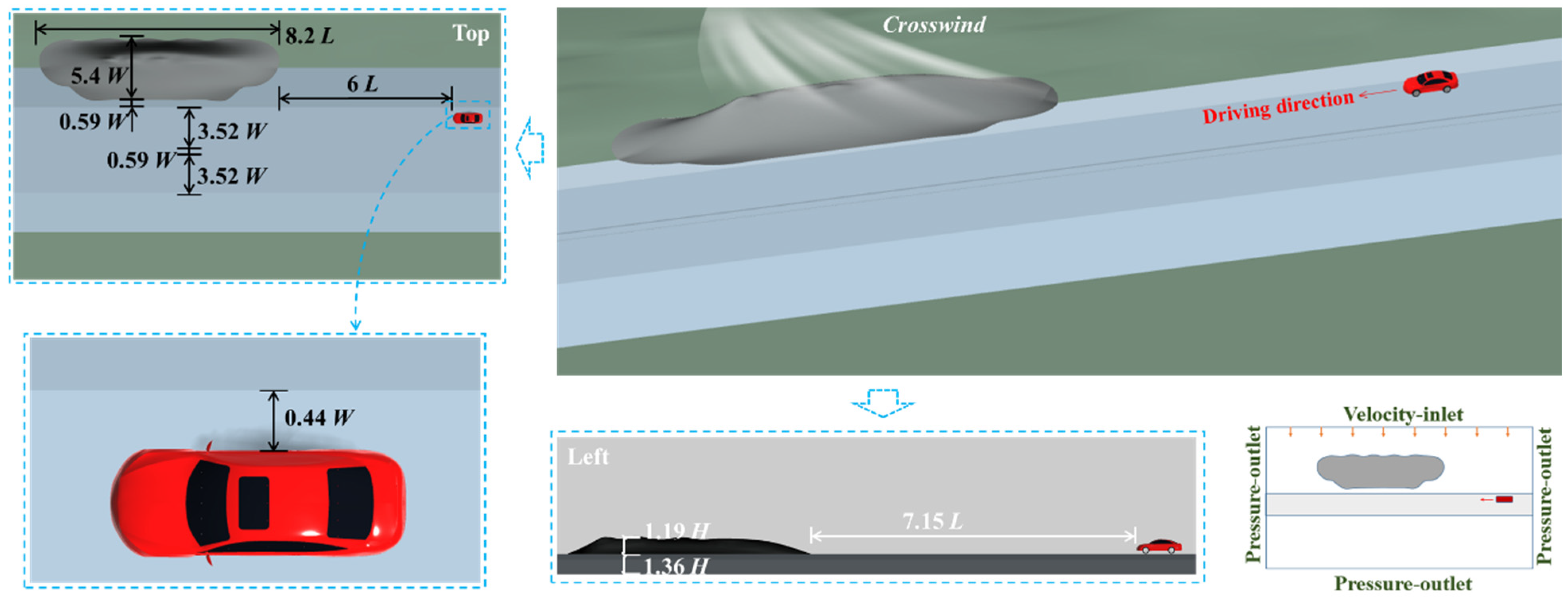
As shown in Figure 1, the geometric model of the sedan is modeled with reference to the shape parameters of a Santana car (manufactured by the SAIC Volkswagen Automotive Co., Ltd. in Shanghai, China), and the door handles and the wheel hubs are appropriately simplified. The sedan has an overall length (L) of 4.48 m, a maximum width (W) of 1.71 m, and a height (H) of 1.47 m.
A mapping drone featuring an Elf 4RTK SE, equipped with an ultra-high-resolution camera that boasts a 1:20,000-pixel CMOS sensor (manufactured by the SZ DJI Technology Co., Ltd. in Shenzhen, China), is employed to capture the topographical features of the designated area, and the obtained topographic data are imported into Rhino 7 for 1:1 modeling. Figure 2 illustrates the geometric details and the boundary conditions for the computational domain, with specifics regarding its dimensions and boundaries available in the literature [30]. The dune dimensions are as follows: a length of 8.2 L, a width of 5.4 W, and a height of 2.55 H. Additionally, the dune is situated 0.59 W away from the roadway’s edge. The cross-section of the road is designed as a four-lane road in both directions, and the lanes in the different driving directions are separated by a 0.59 W wide central divider. The width of the roadway in each driving direction is 3.52 W, the height from the ground is 1.36 H, and the slope of the side slope is 1:3. The initial position of the sedan is 6 L from the edge of the dune in the driving direction and 0.44 W from the edge of the road, and the speed of the sedan is 27.78 m/s.

2.2. Details of Meshs and Calculations

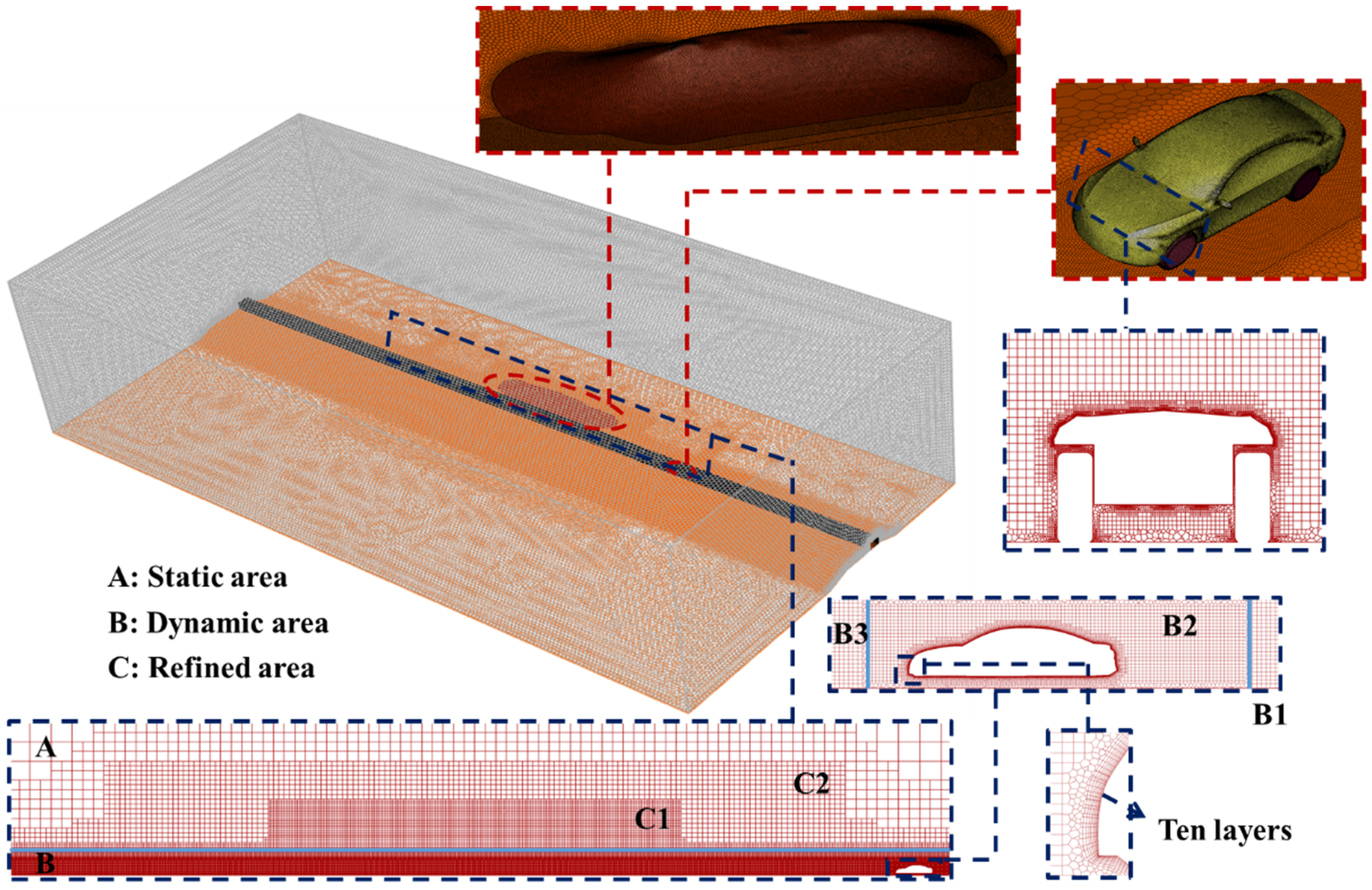
On the basis of the “mosaic” mesh technique, the computational domain of the model is meshed with a poly-hexcore mesh, and the final numbers of mesh cells for the two mesh models are approximately 46 and 71 million. Here, a mesh model comprising 46 million elements is utilized for the RNG k-ε and IDDES simulations, while a mesh strategy with a total of 71 million elements is adopted in the LES computational model. This choice is based on the work in Section 2.5. Figure 3 presents the mesh model with a total number of meshes of 46 million in the IDDES method, and the zone away from the train is defined as the static mesh zone (A). In the dynamic zone (B), it is categorized into the fluid area (B2) adjacent to the sedan, the leading area (B1), and trailing layup areas (B3). The flow field data exchange is facilitated through the creation of interfaces between these zones. In the static zone, the smooth transition of the mesh size is realized by establishing two encrypted zones (C). The mesh sizes of encryption zones C1 and C2 do not exceed 0.014 H and 0.034 H, respectively, and the mesh size in the most external zone is approximately 0.14 H. The mesh size of the dune and the embankment is controlled within 0.034–0.068 H, and 10 boundary layers are set on them.
In the dynamic mesh zone, the majority of the area near surface of the sedan is occupied by a positive polygonal mesh, with an approximate size range of 6.81 × 10⁻⁴–1.36 × 10⁻³ H. Ten of the attached layers are set up on sedan surfaces (estimated, y+ < 1). The y+ value is used to distinguish the different velocity laws exhibited in different regions close to the wall in a turbulent flow. For the IDDES method, it is recommended to target a y+ value within the range of 1 to 5 for the near-wall mesh cells. In practice, employing a y+ value of around 1 for the IDDES simulations is often favored because it provides more accurate results in the near-wall region. However, a slightly higher y+ value, around 5, can still maintain acceptable accuracy while reducing computational cost. In addition, to capture the flow characteristics near the wall, LES models generally require y+ values close to 1. In the RNG k-ε model, wall-modeled turbulence modeling approaches generally require 30 < y+ < 300. Equations (1) and (2) provide the formulae for estimating the y+ value.
y + = u y ν
u = τ ω ρ
where u , ν , and ρ are the friction velocity at the nearest wall (unit: m/s), the local kinematic viscosity (value: 1.8 × 10⁻⁵ Pa/s), and the density (value: 1.225 kg/m3) of the fluid, respectively; τ ω and y represent the wall shear stress (unit: Pa) and distance to the nearest wall (unit: m), respectively.
Table 1 presents the main parameter settings of the cases in this study. All simulations are conducted using a transient calculation method, with the crosswind velocity uniformly set at 20 m/s and the sedan’s driving speed at 27.78 m/s. The time steps of the calculation are maintained at 5 × 10⁻⁴ s, and the Courant number is 0.694. Computational models are computed by commercial solvers, and the process is carried out at the Wuxi Supercomputing Center in China, using 144 cores for each model, taking a total of 26 days. The computation times of all cases are presented in Table 1.

2.3. RNG k-ε, LES, and IDDES Theory

The turbulence modeling approach is a closed set of equations describing the mean values of turbulence on the basis of the Reynolds average equation of motion and the pulsating equation of motion, which rely on the combination of theory and experience and introduce a series of model assumptions. The RNG k-ε, LES, and IDDES modeling theory are proposed based on the Reynolds-averaged Navier–Stokes equations (Equations (3) and (4)).
ρ t + ( ρ u i ) x i = 0
( ρ u i ) t + ( ρ u i u j ) x j = p x i + σ i j x j + ( ρ u i u j ) x j
where u i and u j denote the Reynolds-averaged velocity component with the averaging sign omitted; ρ and p are the fluid density and pressure, respectively; u i is the pulsation velocity; and σ i j is the stress tensor component. The k-ε model is the most widely used turbulence modeling approach in flow computation, including three forms (Standard k-ε, RNG k-ε, and Realizable k-ε), and their governing equations can be found in the literature [31]. Compared to the standard k-ε model, the RNG k-ε models developed based on reformed group theory add an extra factor (Equations (5) and (6)) to the ε equation and consider the influence of eddies on the turbulence. Thus, the RNG k-ε model demonstrates superior performance compared to the standard k-ε model in terms of computational accuracy for high-velocity flows, vortex dynamics, and regions close to walls [32,33,34].
t ( ρ k ) + x i ( ρ k u i ) = x j ( α k μ e f f k x j ) + G k + G b ρ ε Y M + S k
t ( ρ ε ) + x i ( ρ ε u i ) = x j ( α ε μ e f f ε x j ) + C 1 ε ε k ( G k + C 3 ε G b ) C 2 ε ρ ε 2 k R ε + S ε
where u and μ e f f denote the flow velocity and the effective turbulent viscosity, respectively; ρ , ε, k, and R ε are the fluid density, the dissipation rate, the turbulent kinetic energy, and the extra factor, respectively; G k is the turbulent kinetic energy generation term caused by the average velocity gradient; G b is the turbulent kinetic energy generation term caused by the buoyancy force; Y M denotes the influence of the turbulent pulsating expansion on the total dissipation rate; S k and S ε are user-defined source terms; C 1 ε , C 2 ε , and C 3 ε are empirical coefficients; α k and α ε are the reciprocals of k and ε effective Prandtl numbers, respectively.
In a non-stationary turbulent field, large-size vortices dominate the evolution of the flow field, while small-size vortices mainly cause the diffusion of turbulent momentum and are significantly isotropic. The LES method filters the real velocity field u i ( x i , t ) through a filtering procedure, which resolves only the large-scale turbulence structure, and then selects an appropriate model to solve for the small-scale turbulence. LES methods are able to capture more of the turbulent large-scale motion than RNG k-ε methods. The filtering process is defined as Equation (7), and then linear eddy viscosity models are employed to link the sublattice stresses to the resolved strain rate tensor (Equation (8)).
U ¯ i ( x i , t ) = G ( r , x i ) u i ( x i r , t ) d r
τ i j R 1 3 τ k k R = 2 ν S G S S ¯ i j = ν S G S ( U ¯ i x j + U ¯ j x i )
where G ( r , x i ) and τ i j R are the filter function and the sublattice scale stress tensor, respectively; scale factor ν S G S indicates the vortex viscosity of the sublattice motion; and U ¯ i and U ¯ j denote velocities obtained from the filtered decomposition.
In the detached eddy simulation (DES), the zones near the sedan’s surface are calculated using the RNG k-ε method, while the fully developed zone of turbulence away from the sedan’s surface is calculated using the LES method. Consequently, the DES method can notably reduce the number of meshes surrounding the sedan, thus reducing the computational costs while ensuring computational effectiveness. When using the DES model to predict the wind field, Risan et al. found that the measured results on the leeward side of hilly terrain differed from those predicted by the DES model [35]. They attributed this to the improper definition of the boundary layer mesh length, which resulted in the problem of unphysical separation and logarithmic mismatch between the boundary layers. Over the years, researchers have continuously improved and optimized the DES model. The Delayed Separation Eddy Simulation (DDES) method can avoid the separation phenomenon by controlling the parameters of the boundary layer [36]. In addition, the IDDES method has been developed based on DDES to deal with the logarithmic mismatch between the layers. Therefore, the IDDES method based on SST in the RANS model has been identified in this study. In the IDDES method, the scale of length is evaluated by Equation (9):
l = f d ( 1 + f e ) l R A N S + ( 1 f d ) l L E S
where f e and f d denote the lifting and hybrid functions, respectively; and l R A N S and l L E S denote the length scale of the RANS and LES models, respectively.

2.4. Calculation Strategy

DPM is employed to study the dynamics of multiphase flows involving combinations of gas–liquid, gas–solid, liquid–solid, and gas–liquid–solid interactions. It carries out Lagrangian trajectory calculations for the dispersed phases such as particles, droplets, or bubbles, along with their interaction with the continuous phase. Multiphase flow scenarios encompass a variety of applications like channel flows, sprays, sedimentation processes, separation techniques, and cavitation phenomena. For the purpose of evaluating and comparing the computational efficacy of three different turbulence modeling approaches in analyzing the aerodynamic response of a sedan moving through a dune section within a wind–sand flow environment, this study utilizes the DPM to model the wind–sand flow dynamics. In this method, sand particles are injected into air, and the Eulerian–Lagrangian approximation is used to calculate the air–sand interaction. Equation (10) presents the equilibrium equations of a sand particle in the air stream.
m p d u p d t = F g + F d + F l + F m + F b
where F g , F d , F l , F m , and F b are gravity, drag, Saffman lift, Magnus, and Brownian forces, respectively; m p is the mass of a sand particle; and u p is the velocity of the particle.
The aerodynamic loads (aerodynamic drag Fx, aerodynamic lift Fy, lateral force Fz, rolling moment Mx, yaw moment My, and pitching moment M) of the sedan are obtained by integrating the forces or moments subjected to several calculation segments. The corresponding calculation strategies and formulas can be found in the literature [25]. Among these loads, aerodynamic loads that lead to the yaw, sideslip, and roll behaviors of the sedan are the Fz, Mx, and My [13]. To capture the aerodynamic forces acting on the sedan as it moves, the surface mesh cells of the sedan serve as the computational domain’s boundary faces. The transient pressures exerted on these surface cells are integrated and computed in real-time through the implementation of a tailored UDF program.
To compare and analyze the sedan’s aerodynamic loads in different cases, the lateral force coefficient Cz is obtained by dimensionalizing the lateral force Fz using F′. The rolling moment Mx and yaw moment My are dimensionless, using M′ to obtain the rolling moment coefficient Cmx and yaw moment coefficient Cmy. The calculation equations for F′ and M′ are shown in Equations (11) and (12). Equation (13) is used to add dimension to the pressure on the sedan surface.
F = U s 2 S ρ / 2
M = U s 2 S H ρ / 2
C p = 2 ( p j p 0 ) ρ U c 2
where U s and ρ denote the sedan’s running speed and the atmospheric density, respectively; and S and H denote the side area and height of the sedan, respectively. U c and C p represent the velocity of the crosswind and the pressure coefficient on the surface of the car, respectively.

2.5. Independence of the Mesh

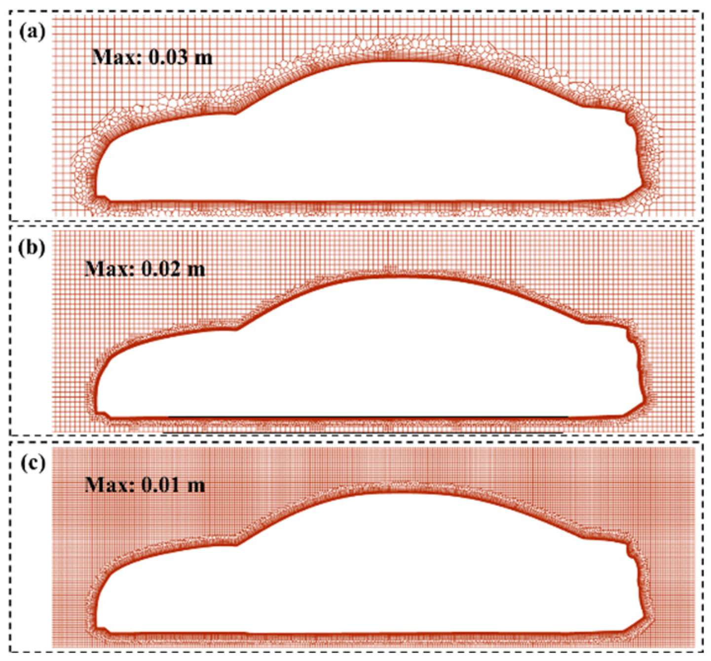
To analyze the effect of different grid resolutions upon computational results, three mesh resolution levels (Coarse, Medium and Fine) were established by varying the parameters of the mesh size in the encrypted zone (C). The RNG k-ε and IDDES models were both calculated using an identical group of mesh models (Figure 4), and the amounts of mesh units applicable to the RNG k-ε and IDDES models were 36 million (Coarse), 46 million (Medium), and 54 million (Fine), respectively. The amounts of mesh units for the LES models with different mesh resolutions were 59 million (Coarse), 71 million (Medium), and 81 million (Fine), respectively. All the models were solved by referring to the computational strategies presented in Section 2.2 and Section 2.4.
The lateral force of the sedan is used as a monitoring index, and Figure 5 presents the temporal variation in the lateral force coefficients for the sedan as obtained by the RNG k-ε, LES, and IDDES models. “Coarse”, “Medium”, and “Fine” are denoted by the abbreviations “C”, “M”, and “F”, respectively. The results show that the predictions from the RNG k-ε (M) model are largely in alignment with the RNG k-ε (F) model, with a discrepancy in the variation amplitude of lateral force of less than 2.3%. The difference between the maximum fluctuation in lateral force obtained from the LES (M) and the corresponding value from the LES (F) model is controlled within 3.3%. The maximum value of the difference between the results obtained from the IDDES (M) model and the corresponding value from the IDDES (F) model is only 0.8%. Finally, the reasonable numbers of mesh units for RNG k-ε, LES, and IDDES models are identified as 46, 71, and 46 million, respectively.

2.6. Field Experiment Verification

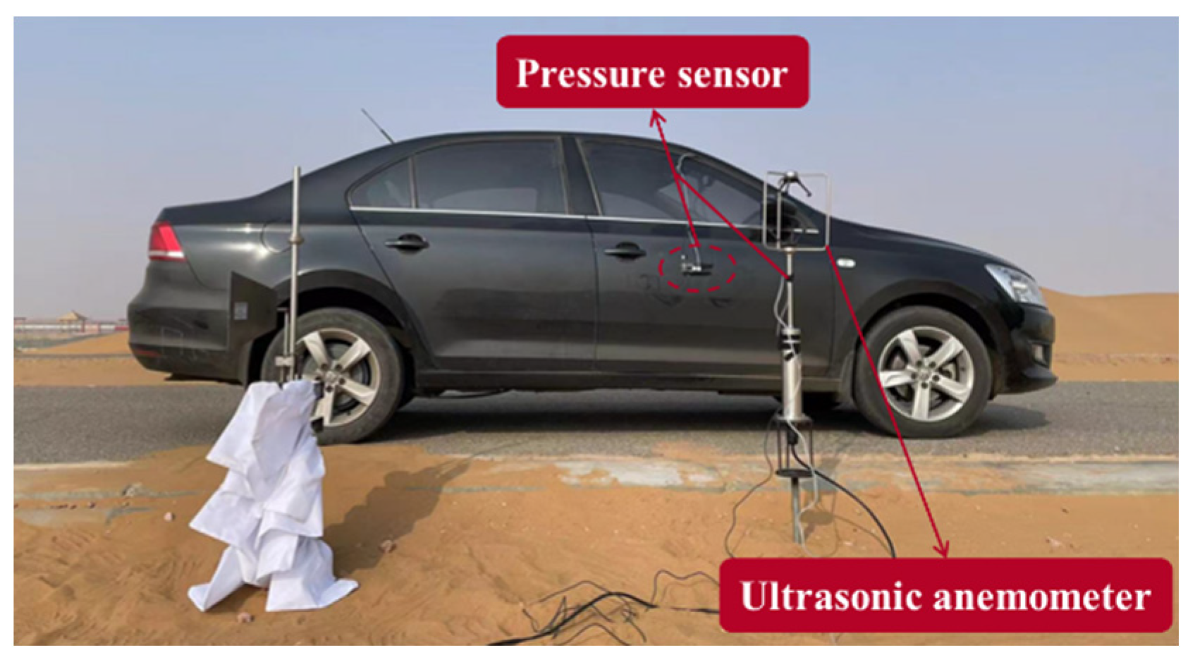
To verify the reliability of the CFD methods used in this study and their results, a series of field tests were carried out on the wind speed and pressure at a desert road. Three-cup anemometers and wind vanes were employed for the extended monitoring of wind speed and direction in the dune section. As shown in Figure 6, the sedan was running at 16.67 m/s without crosswinds, and a micro differential pressure sensor was used to monitor the pressure change in the surface of the passenger door. The passage of a sedan through a dune section induces disturbances in the surrounding flow field, resulting in fluctuations and an increase in wind speeds and pressures along the roadside, proportional to the sedan’s speed. The presence of sand on the surface of the desert highway exacerbates the issue, as the dust stirred up by the sedan’s wake during passage adversely affects individuals and facilities along the roadside. Therefore, a pressure measurement point and an ultrasonic anemometer, Gill Wind Master Pro (manufactured by GILL in the Lymington, UK), are installed at the 0.9 m height of the road shoulder at the end of the dune. The corresponding CFD models are built according to the field conditions, and the differences between the field test results and the corresponding CFD prediction results are compared.
Figure 7 presents the time history curves of the pressure at a measurement point on the sedan surface obtained from the field test, the RNG k-ε, LES, and IDDES models. The differences between the sedan surface pressures predicted by the RNG k-ε, LES, and IDDES models (−36.16, −37.46, and −36.94 Pa) and the corresponding values in the field (−39.18 Pa) are 7.7%, 4.4%, and 5.7%, respectively, and the fluctuations range roughly between −20 and −60 Pa. Therefore, the surface pressures on the sedan as forecasted by the LES model align more closely with the field test data compared to those predicted by the RNG k-ε and IDDES models. Comparing the fluctuation amplitudes of pressures at the measurement point obtained by three turbulence modeling approaches with the corresponding results obtained from the field test during the time period of 0–2.5 s, it can be found that the fluctuation amplitude (33.15 Pa) of the pressure obtained based on the IDDES model is the closest to the corresponding result (58.5 Pa) of the field test. This discrepancy cannot be ignored, and further analysis reveals that the results obtained based on the field tests fluctuate substantially between the periods 0–1.0 s and 2.0–2.5 s, which may be attributed to the fact that the speed of the sedan did not stabilize during the starting and stopping periods. After comparing the pressure fluctuations during 1.0–2.0 s obtained based on the three turbulence modeling approaches with the corresponding results of the field tests, it can be found that the fluctuation amplitude (32.27 Pa) of the pressure obtained based on the LES model was the closest to the corresponding result (30.2 Pa) of the field test.
Figure 8 shows the time interval curves of wind velocity and pressure recorded at the point on the road shoulder during the crossing of the sedan. The average results of the 10 reproducible experiments performed in the field tests were obtained and then compared with the corresponding results predicted by RNG k-ε, LES, and IDDES models. As depicted in Figure 8, at the 0.9 m height on the road shoulder, the wind velocity at the point evolves between −1.0 m/s and 0.7 m/s, while the pressure evolves between −12 and 8 Pa. The time interval curves of the pressure and the wind velocity measured at the measured points of the road shoulder are basically consistent with the corresponding results predicted by the CFD models. In the field tests, the variations in wind velocity and pressure at points are recorded as 1.583 m/s and 19.021 Pa, respectively. For the RNG k-ε, the corresponding variations are 1.451 m/s and 17.522 Pa. The fluctuation results predicted by the LES model are 1.497 m/s and 17.783 Pa, respectively. The fluctuations in the corresponding results calculated by the IDDES model are 1.472 m/s and 17.577 Pa, respectively. The LES model’s predictions are found to be more in line with the field test results than those of the RNG k-ε and IDDES models, with discrepancies kept within a 7% margin. Upon comparing the peak wind speed moments, it is observed that the IDDES model’s highest wind speed moments at 1.361 s are closest to the field test results at 1.471 s, with a difference of 7.5%. Similarly, the LES model’s lowest wind speed moments at 1.087 s are nearest to the field test results at 1.012 s, with a variance of 7.4%. Comparing the corresponding moments of peak pressure, it can be seen that the moments (1.015 s, 1.252 s) of maximum and minimum pressure based on the LES model are the closest to the corresponding results (1.068 s, 1.21 s) of the field test (5.0%, 3.5%).
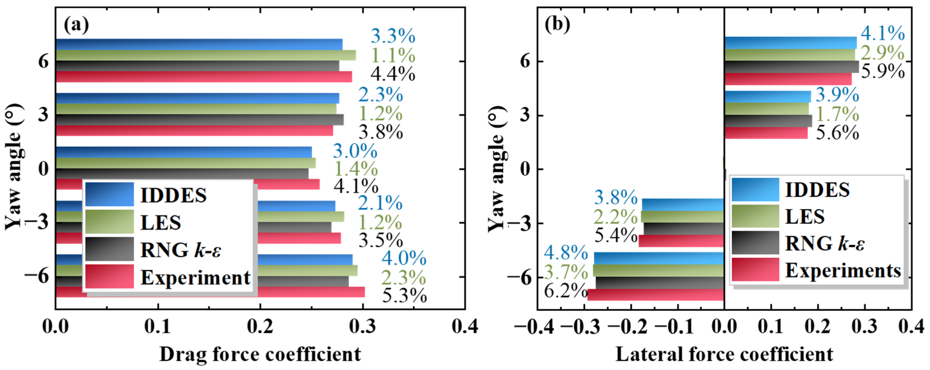
To verify the reasonableness of the aerodynamic load calculation strategy for the sedan in the numerical method, the RNG k-ε, LES, and IDDES models are built based on the numerical method in this study and the wind tunnel tests in the literature [21], and the aerodynamic drag and lateral forces of the sedan are presented in Figure 9. The differences between the aerodynamic load values obtained based on the RNG k-ε, LES, and IDDES methods with the wind tunnel test results are marked in the figure. Under five yaw angle conditions (−6°, −3°, 0°, 3°, and 6°), the differences in the aerodynamic drag of the sedan obtained by the RNG k-ε, LES, and IDDES-based methods with the experimental results are within 5.3%, 2.3%, and 4.0%, respectively. Regarding the lateral forces on the sedan, the differences between the RNG k-ε, LES, and IDDES methods and the tests are within 6.2%, 3.7%, and 4.8%, respectively. Compared to the RNG k-ε and IDDES methods, the aerodynamic loads of the sedan predicted by the LES method are closest to the wind tunnel experiment results.

3. Results

3.1. Aerodynamic Behavior of the Sedan

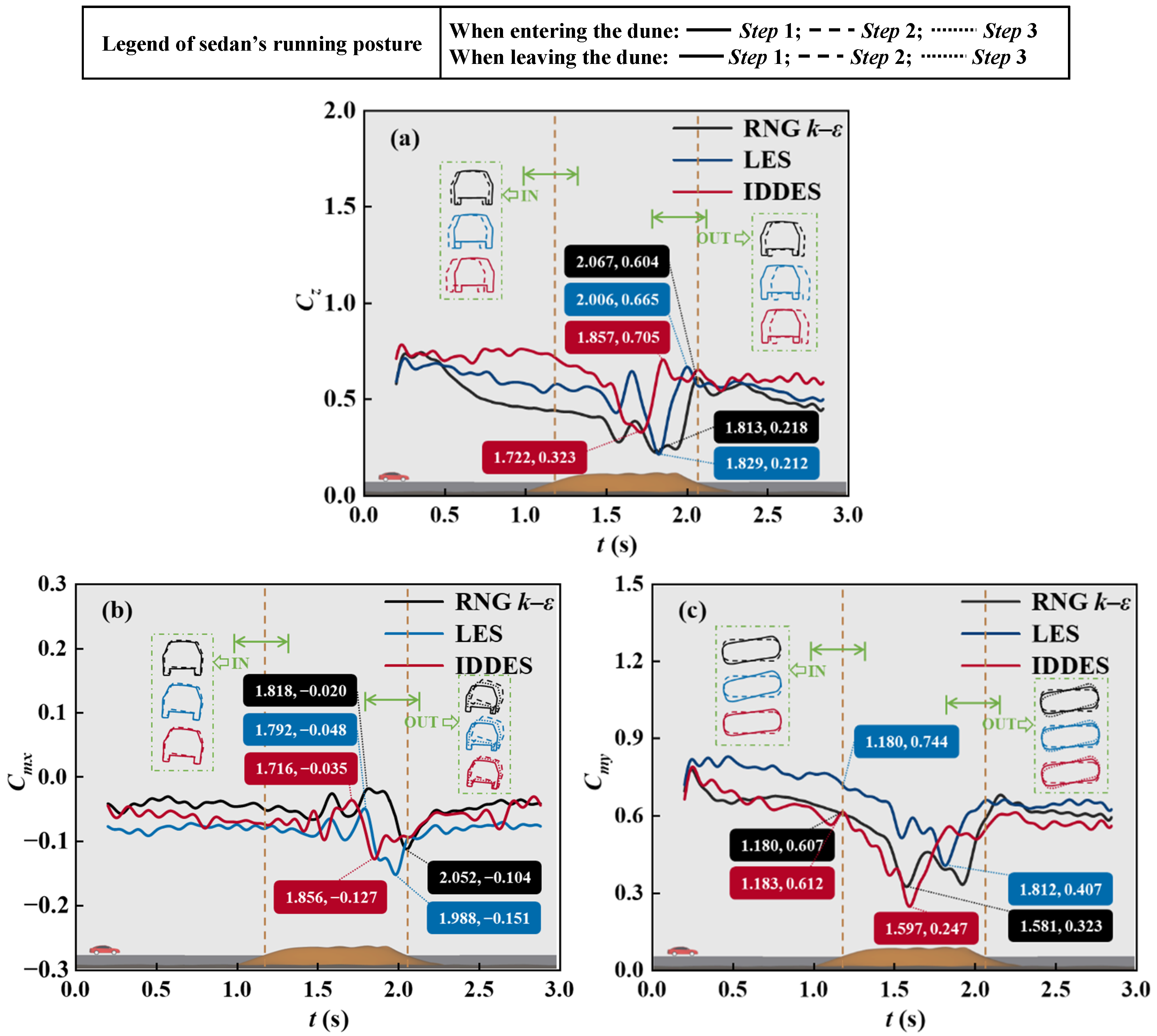
To reveal the effect of various turbulence modeling approaches on computed results, Figure 10 presents the temporal progression of the sedan’s three aerodynamic forces as it traverses the dune at a speed of 27.78 m/s. These predictions are conducted by the RNG k-ε, LES, and IDDES method. The processes of sedan driving into and out of the dune section are marked as “IN” and “OUT”, respectively, and the changes in the running posture of the sedan are drawn according to the variation characterization of aerodynamic forces. The time interval of the sedan driving within the dune section is marked using an orange dashed line. The peak values and variation amplitude of the corresponding aerodynamic loads are provided in Table 2. Section 2.6 verifies that the pressure and the wind speed obtained from the LES model are more consistent with the measured values obtained from the field tests than those from the other models. Therefore, the calculated results of the LES model are used as the benchmark for analyzing the predictive abilities of the RNG k-ε and IDDES methods.
Figure 10 and Table 2 indicate some differences in the temporal laws of the three aerodynamic loads of the sedan predicted by the three turbulence modeling approaches during the sedan crossing of the dune. Regarding the lateral forces, the calculated results based on the RNG k-ε and IDDES models present a certain deviation from those of the LES model. The maximum amplitudes of the fluctuations in the sedan’s lateral forces calculated by the RNG k-ε and IDDES models are 0.067 (14.8%) and 0.071 (15.7%) lower than the LES model, respectively. The maximum fluctuations’ amplitude in the rolling moment coefficients of the sedan predicted by RNG k-ε and IDDES are 0.019 (18.4%) and 0.011 (10.7%) lower than the corresponding values calculated by LES, respectively. The yawing moment on the sedan is underestimated by both the RNG k-ε and IDDES methods in contrast to the LES model. The maximum amplitude of the fluctuations in the yaw moments predicted by RNG k-ε is 0.053 (15.7%) lower than the corresponding values obtained by LES. The maximum amplitude of the fluctuations in the yaw moment coefficients of the sedan predicted by IDDES is 0.028 (8.3%) higher than the corresponding values obtained by LES.
As shown in Figure 10, there is no significant variation in the sedan’s aerodynamic load coefficients during the “IN” period due to the gentle slope of the dune entrance in the route direction, and the existence of a gentle transition area during the switching of the running scene of the sedan. By contrast, the sudden switching of the running scene of the sedan during the “OUT” period leads to a sharp alteration in the sedan’s aerodynamic load. The sudden shifts in lateral forces could potentially induce a lateral displacement of the sedan, which might result in the sedan veering off its designated travel path. The transient fluctuation in the rolling moments may cause the lateral deflection of the sedan, which will lead to the rolling motion of the sedan. The sudden change in the yaw moments may cause an oscillation of the sedan, making the driving direction of the sedan difficult to control.
The running posture of the sedan during the “OUT” period is more complex than the changes during the “IN” period. Taking Figure 10a as an example, the changes in the running posture of the sedan during both the “IN” and “OUT” periods only go through one phase (i.e., the left movement). However, the change in the running posture of the sedan during the “OUT” period has an abrupt nature compared to that in the “IN” period. In Figure 10b, the running posture of the sedan during the “IN” period goes through only one phase (i.e., right leaning), while the running posture during the “OUT” period undergoes two phases (i.e., from right to left leaning). As shown in Figure 10c, the running posture during the “IN” period goes through one phase (i.e., right bias), and the running posture during the “OUT” period undergoes two phases (i.e., right bias to left bias).
In summary, the discrepancies between the peak variations in the sedan’s aerodynamic loads calculated by the IDDES model and those by the LES model are kept within the range of 8.3% to 15.7%. Furthermore, the discrepancies between the peak fluctuations in lateral force, roll moment, and yaw moment as forecasted by the RNG k-ε method in comparison to the LES model’s calculations fall within 14.8% to 18.4%.

3.2. Pressure Characteristics of the Sedan Surface

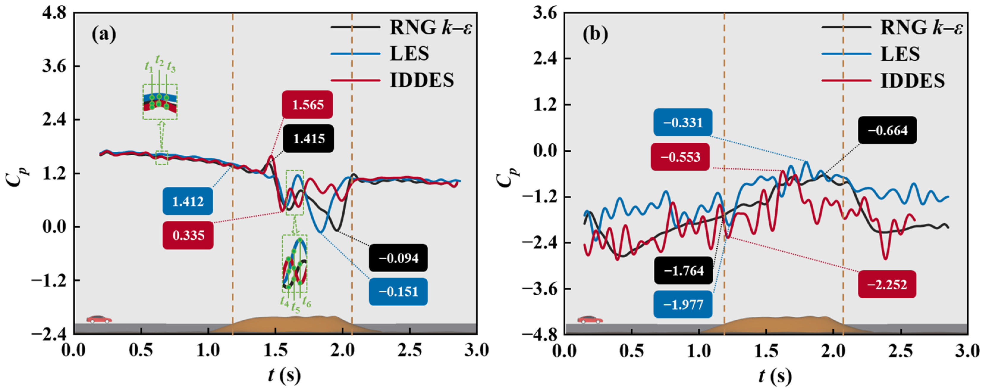
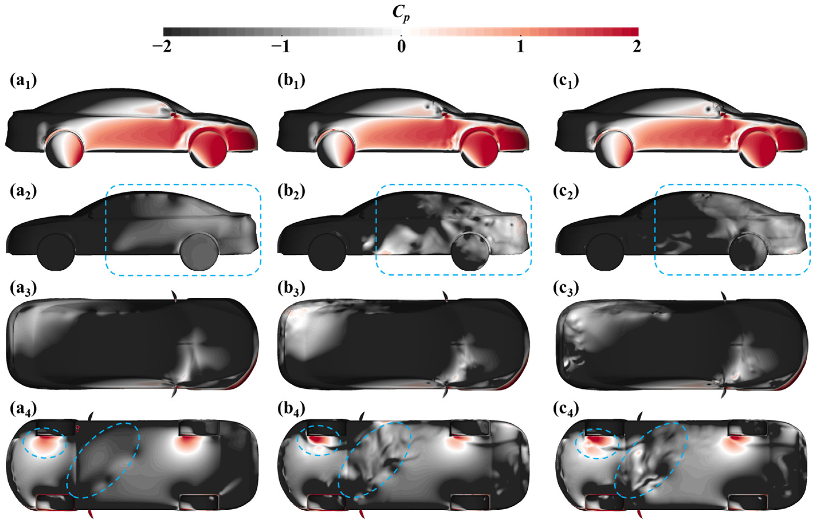
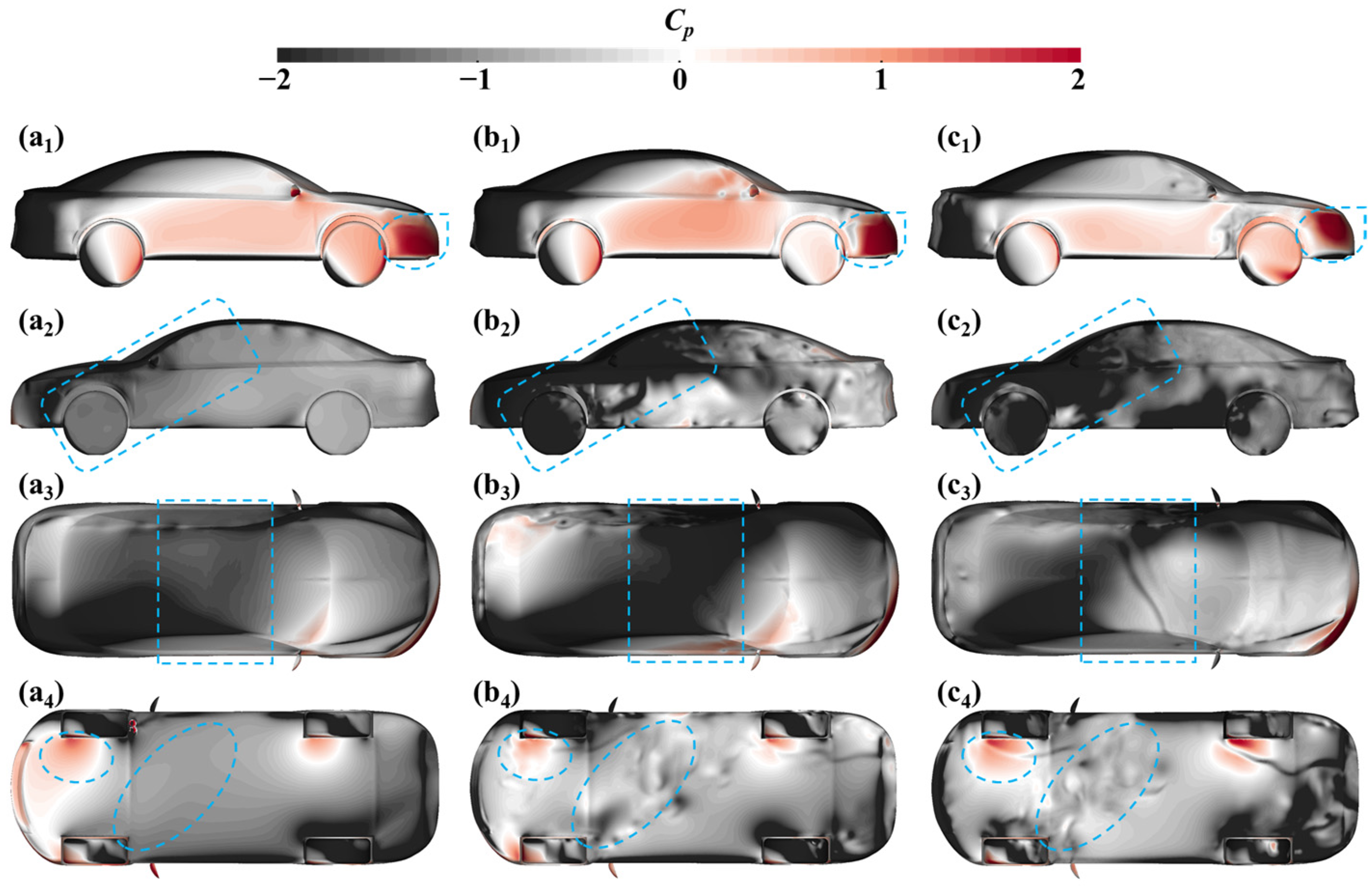
To evaluate the divergence in predictive capabilities among various turbulence modeling approaches concerning the sedan’s aerodynamic load, Figure 11 shows the temporal progression of the pressure coefficient at measurement points on the front door surface, both on the windward and leeward sides of the sedan. Six typical moments (t1, t2, t3, t4, t5 and t6) before and after the sedan drives into the dune are marked in Figure 11, and they are used as the time pitchings for the subsequent study of the transient evolution of the vortex structure. Figure 12 and Figure 13 present the respective distributions of the pressure on the sedan surface before and after (moments t1 and t4) driving into the dune section at the speed of 100 km/h on the basis of turbulence modeling approaches RNG k-ε, LES, and IDDES, and the time interval of the sedan driving within the dune section is marked using an orange dashed line.
As shown in Figure 11a, the prediction results of the three turbulence modeling approaches for the pressure coefficient at the measurement point on the windward of the sedan are consistent at t1. The evolutionary trend in the pressure obtained by three turbulence modeling approaches basically coincides after the sedan enters the dune section, but some deviations in the amplitude of the pressure fluctuations exist. As shown in Figure 11b, the evolutionary trend in the pressure at the measurement points obtained by RNG k-ε model is identical to the LES model, but the RNG k-ε model fails to capture small fluctuations in the pressure. The absolute value of the pressure coefficient at the measured point on the leeward calculated by IDDES is higher than corresponding values calculated by LES. The variation amplitude of the pressure on the windward calculated by the RNG k-ε and IDDES models differs from corresponding values obtained from the LES model by 0.054 and 0.333 (3.45% and 21.3%), respectively, when the sedan is driving within the dune section. Regarding the leeward measurement points, the variation amplitude of the pressure coefficient in the RNG k-ε and IDDES simulations differs from those in the LES by 0.546 and 0.053 (33.17% and 3.22%), respectively.
As shown in Figure 12, the results obtained by the RNG k-ε, LES, and IDDES models regarding the pressure distribution on the top and windward surfaces of the sedan at time t1 are almost the same. However, the predictions made by these three models for the pressure distribution on the leeward surface of the sedan show some variations. In the RNG k-ε simulation, a large negative pressure zone is observed in the head of the leeward, failing to represent the detailed features of the pressure distribution in the middle and tail areas. Although the IDDES model captures the differences in the pressure distribution between the small areas at the rear doors on the leeward, it is less capable of describing the differences in more detail than the LES model. According to the results predicted by LES and IDDES, a strip of negative pressure zone is observed in the bottom center of the sedan, and a positive pressure zone divided into two regions is observed in the leeward of the wheel. This phenomenon is caused by the combination of the crosswind incoming flow and the fluid along the moving direction of the sedan. At t4, the RNG k-ε model only acquires the rough pressure distribution at the leeward and bottom surface of the sedan and does not capture the details of the local pressure distribution pattern (Figure 13). Both the LES and IDDES models capture the details of the local pressure distribution patterns on the sedan surface, but the LES model has a more detailed descriptive capability.
In general, the three turbulence modeling approaches can accurately predict the pressure on the windward of sedan when they pass by a dune. The pressure at the measurement point on the leeward obtained by the IDDES model is higher than the LES model (Figure 11b). Thus, the pressure differential between the windward and leeward sides of the sedan is significant, which leads to the underperformance of the sedan’s lateral force predicted by the IDDES model (Figure 10a). As shown in Figure 13(b2,c2), the negative pressure regions on the leeward surface of the sedan, as projected by the RNG k-ε and IDDES models, tend to shift towards the rear when contrasted with the LES model’s predictions. The action points of the sedan’s lateral forces move backward, resulting in the small yaw moment of the sedan calculated by the RNG k-ε and IDDES models (Figure 10c). The aerodynamic loads of the sedan are obtained by integrating the aerodynamic pressures (moments of pressure against the gravity center of the sedan) of mesh cells near the sedan’s surface. The leeward side of the sedan experiences reduced negative pressure in the RNG k-ε model when compared to the LES and IDDES models, leading to a reduction in the sedan’s differential pressures. Consequently, the aerodynamic forces calculated by the RNG k-ε model are less than those derived from the LES and IDDES simulations. The RNG k-ε model relies on the RANS equations for simulating turbulence, which forecasts the mean behavior of turbulence by solving the equations for turbulent kinetic energy (k) and its dissipation rate (ε). The core content of the RANS equation is the Reynolds averaging of the flow field, which means that the variables of the flow field are decomposed into the mean and pulsation components. Therefore, the RANS equations cannot directly account for the time-varying effects and irregularities in turbulence, and it is difficult to capture the transient effects due to the evolution of turbulent structures [29,37].

3.3. Transient Characteristics of the Flow Field

3.3.1. Wind Speed

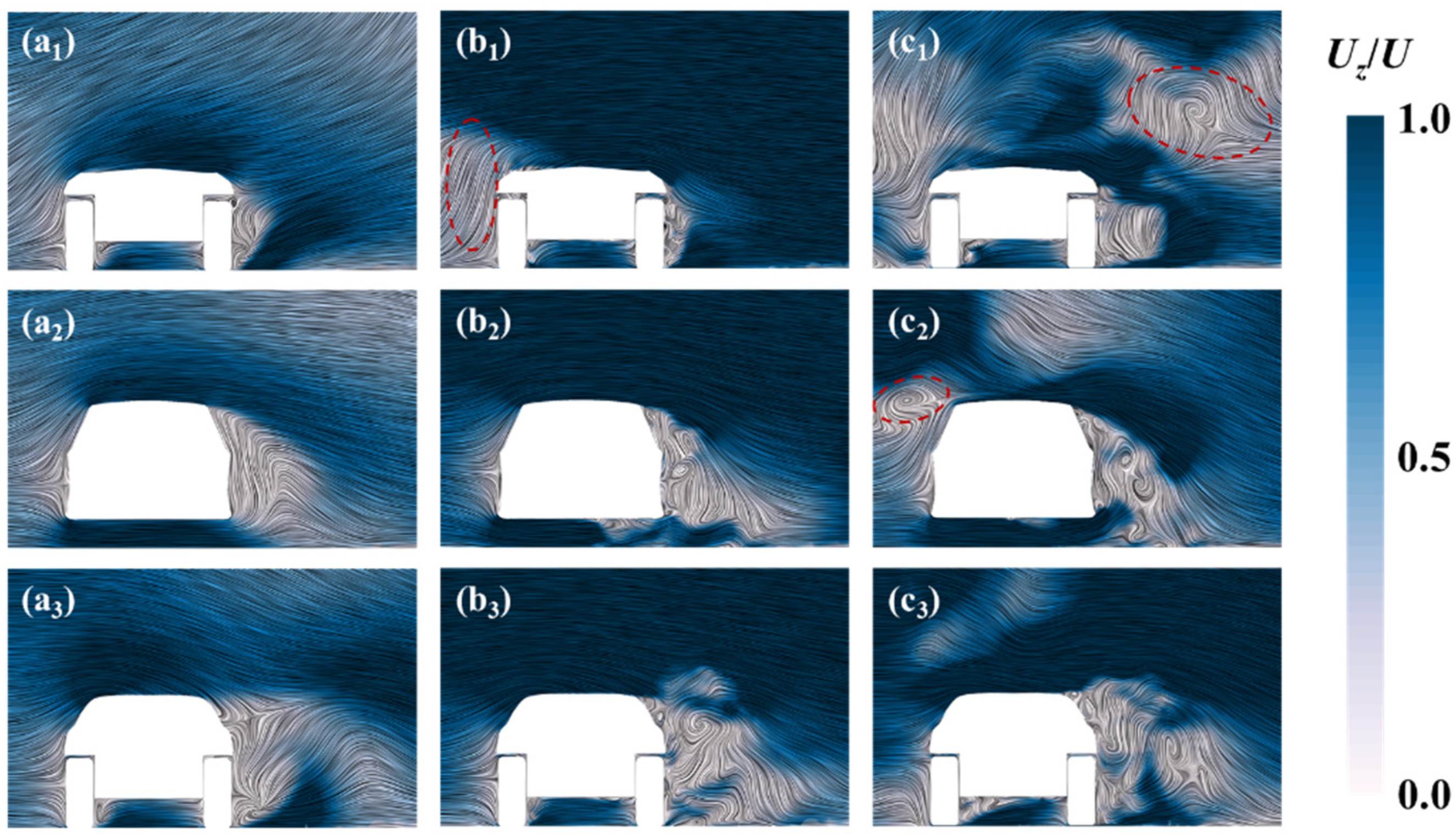
Figure 14 and Figure 15 present the flow fields of three typical cross-sections (the front wheels, the middle of the sedan, and the rear wheels) of the sedan at t1 and t4 on the basis of the RNG k-ε, LES, and IDDES simulations. The Z component of the wind speed is used for coloring and is dimensionless using the wind speed set at the velocity inlet (U = 20 m/s).
Figure 14 shows various vortex patterns on the leeward of the sedan, as depicted by the three turbulence modeling approaches prior to the sedan’s entry into the dune area (at time t1). The LES and IDDES models describe the turbulent motion on the leeward of the sedan more finely than the RNG k-ε model. As shown in Figure 15, the incoming wind speed decreases significantly on the windward and top of the sedan in the three models after the sedan enters the dune (t4). Compared with the predicted results of the RNG k-ε model, more detailed variations in the wind speed are observed on windward of the sedan based on the LES and IDDES models, and several large vortex structures are also observed on the leeward. This result is due to the frequent vortex shedding of the uniform crosswind incoming flow passing the dune boundary, and the vortex structure shedding at the shear layer continuously develops on the leeward of the dune, leading to the significant non-stationary characteristics on the leeward of the dune.
In summary, the RNG k-ε model successfully anticipates turbulence on the leeward side of the sedan, but only captures a few large vortices. Therefore, the RNG k-ε model cannot predict the small fluctuation characteristics of the sedan’s aerodynamic load. For the LES and IDDES models, the detailed features of the fine vortex structure can be captured on the leeward of the sedan, which reflect the subtle changes the sedan’s surrounding flow field. These vortex structures are progressively detached from the shear layer due to crosswinds, resulting in the fluctuating aerodynamic loads of the sedan.

3.3.2. Evolution of the Vortex Structure

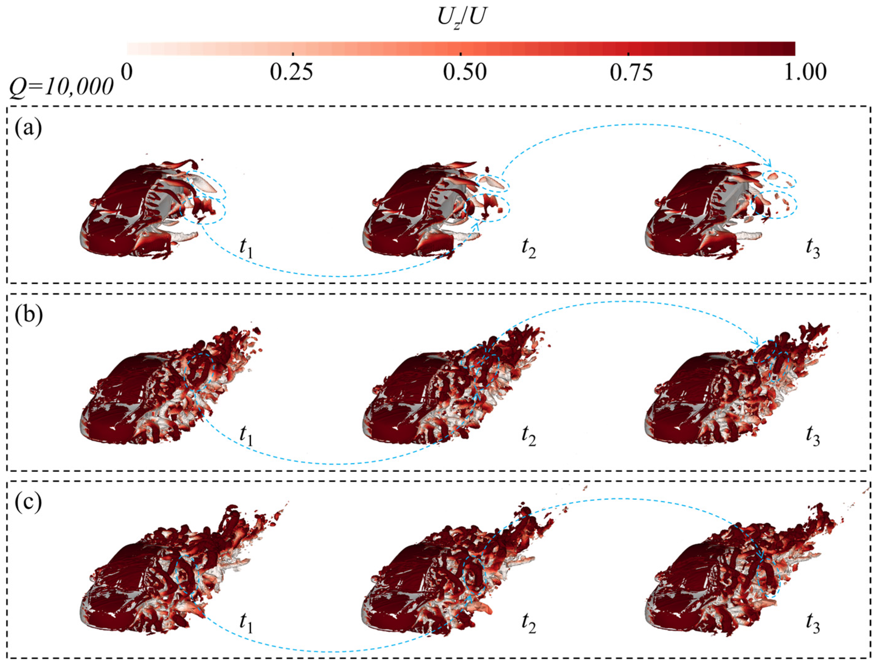
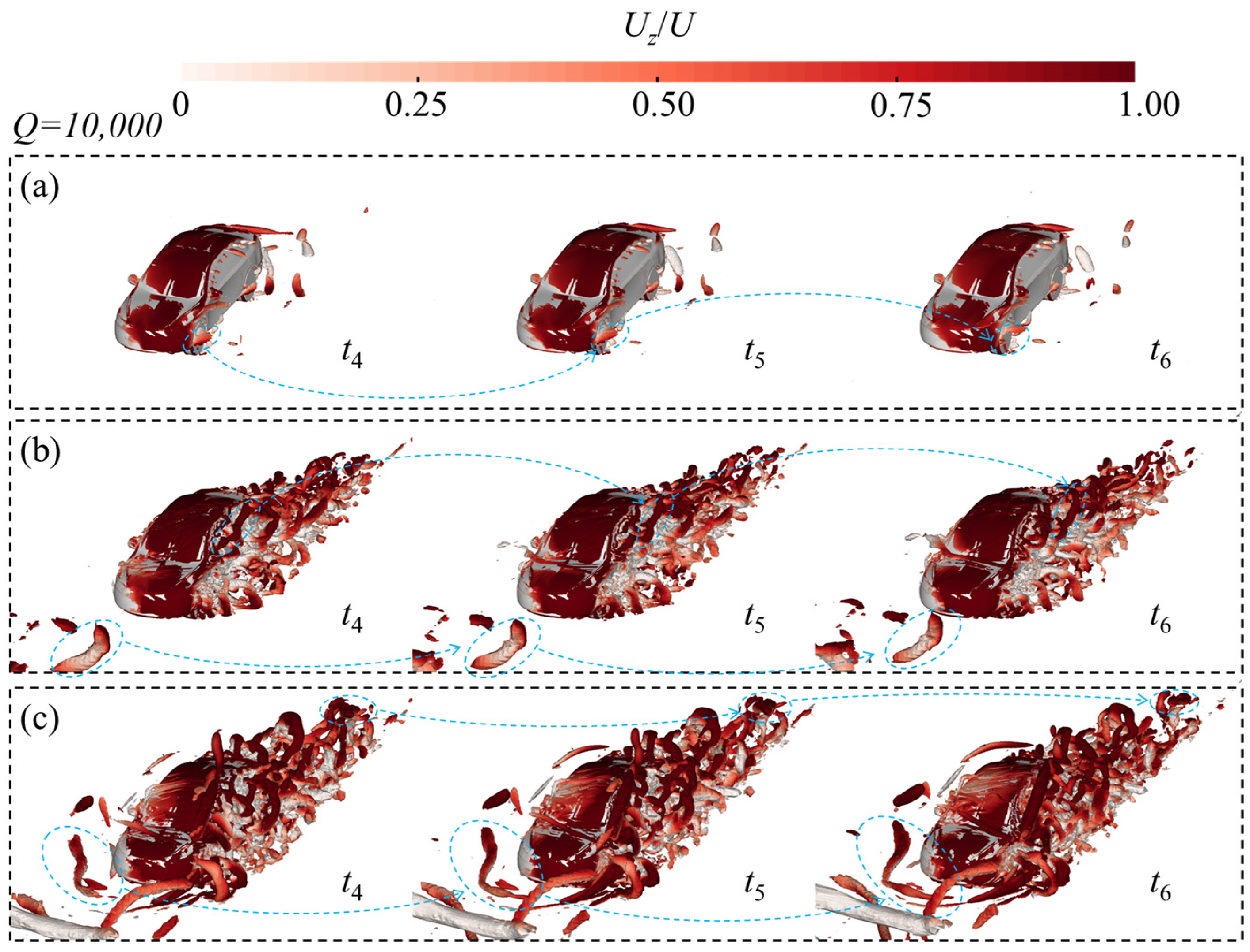
This section further reveals the differences in the predictive ability of different turbulence modeling approaches in terms of the evolutionary characteristics of the vortex structure around the sedan. Figure 16 and Figure 17 present the evolution characteristics of the vortex structure predicted by three turbulence modeling approaches for time periods t1t3 and t4t6, respectively (Q = 10,000). The progression of the vortex structures is highlighted in the figure with a blue dashed line, and the Z-axis component of wind speed is utilized for coloring, which is normalized based on the wind speed specified at the velocity inlet (U = 20 m/s). Six typical moments (t1, t2, t3, t4, t5, and t6) are introduced in Section 3.2.
As shown in Figure 16a, only a few large vortex structures are captured during t1t3 based on the RNG k-ε model. The large vortex structure shedding from the edge of the sedan gradually split into several small vortices, and the vortex structures’ evolution determines the main features of the flow field and the corresponding fluctuation law of the aerodynamic loads. As shown in Figure 16b, many fine vortex structures and lateral vortex structure branches on the leeward of the sedan are described by the LES turbulence modeling approach. The vortex structures continuously detach from the sedan’s rear and leeward side under crosswinds, resulting in fluctuations in the sedan’s aerodynamic loads. The two vortex structures marked in the figure develop toward different directions; one vortex structure develops toward the rear of the sedan, and the another moves toward the lateral direction. On the basis of the IDDES turbulence modeling approach, numerous detached vortex structures are observed on the sedan’s rear and leeward side (Figure 16c), which are mainly large vortex structures. The detached vortex structures continuously break up toward the rear side of the sedan. The vortex structure causes the leeward of the sedan to be subjected to negative pressure. However, the windward of the sedan is affected by the positive pressure, and the difference in pressure between the windward and leeward of the sedan generates lateral force.
After the sedan drives into the dune section, the running scenario of the sedan switches from a uniform incoming flow state to an unsteady turbulent state, and the RNG k-ε model captures few vortex structures (Figure 17a). The vortex structure shedding near the front tire of the sedan gradually ruptured, and the small vortex structure formed with the rupture is not observed in the figure. This phenomenon indicates that the RNG k-ε model has an insufficient ability to capture small vortex structures and an inferior ability to describe the turbulent motion. The RNG k-ε model does not capture small vortex structures and cannot accurately predict the subtle changes in the flow field and present the pulsation effect of the corresponding aerodynamic loads. The RANS equations used in the RNG k-ε method adopt a statistical averaging method in turbulence, which ignores the effects of scale coupling in turbulence. There are multiple scales of vortex structures in turbulence, ranging from large-scale vortices to small-scale turbulent structures that play an important role in the flow. However, the RANS equation focuses only on large-scale structures and averages out the effects of small-scale structures, resulting in an inability to fully capture the interactions between scales and energy transfer in turbulence [38]. As shown in Figure 17b, the vortex structure shedding at the boundary of the dune after the sedan drives into the dune continuously evolve. Thus, large vortex structures are presented in front of the sedan. The marked large vortex structures are approximately the same height as the sedan and move toward the side and rear of the sedan. In Figure 17c, the IDDES model captures many large vortex structures in front and on top of the sedan after it drives into the dune. This phenomenon reflects the pulsating features of the flow field on the dune’s leeward side under crosswinds. Comparing Figure 17b,c, the LES model captures the vortex structures at the head of the sedan, but their number is less than the corresponding results predicted by the IDDES model. This may be caused by the difference between the vortex development states on the leeward side of the sand dune during the continuous moment, and this phenomenon does not prove that the prediction performance of the LES model is worse than that of the IDDES model.

3.4. Wind–Sand Flow

To reveal the difference in the sedan’s aerodynamic characteristics when crossing the dunes under crosswinds and wind–sands, the IDDES method and the DPM technique were used to calculate the aerodynamic force and moment of the sedan under crosswinds and wind–sands. The running speed of the sedan and the crosswind speed are constant at 27.78 m/s and 20 m/s, respectively.
Figure 18 provides the time interval curves of the lateral force, rolling moment, and yaw moment coefficient of the sedan under crosswinds and wind–sands. Table 3 presents the peak values and the fluctuation amplitudes of the lateral force, rolling moment, and yaw moment of the sedan when passing by the dune. The combination of Figure 18 and Table 3 shows that the aerodynamic loads of the sedan under crosswinds and wind–sands have small differences. The lateral force of the sedan decreases under wind–sands compared with that at the crosswind condition. The difference between the fluctuation amplitudes of the lateral force in the wind and wind–sand cases is 0.032 (8.4%). This difference is caused by the sand particles that consume the flow energy, which leads to a decrease in the wind speed of the crosswind and consequently affects the sedan’s aerodynamic loads. In the wind–sand case, the rolling moments of the sedan are generally identical to the corresponding values in the wind case. In the wind and wind–sand cases, the difference in the fluctuation amplitude of the rolling moment is 0.001 (1.1%). In addition, the yaw moments of the sedan do not show any downward impulse, and the sedan is continuously subjected to a stable positive yaw moment. The comparison of the wind and wind–sand cases show a difference in the fluctuation amplitude of the yaw moment of 0.052 (14.2%). This difference is caused by the change in the pressure distribution on the surface of the sedan when passing by the dune.

4. Conclusions

This study verifies that the LES model has an accurate prediction capability of the sedan’s aerodynamic characteristics when it is passing by a sand dune under crosswinds on the basis of field tests. The differences in the aerodynamic loads (lateral force, rolling moment, and yaw moment) of the sedan obtained by the RNG k-ε and IDDES models were compared using the corresponding results obtained by the LES model as the benchmark. The computational cost of the LES model combined with the DPM technique is expensive, and the accuracy of computational results of the IDDES model are near those of the LES model. The calculation time for the LES and IDDES models increased by 60.0% and 11%, respectively, compared to the RNG k-ε model. Finally, the effect of the wind–sands on the sedan’s aerodynamic loads was discussed in conjunction with the IDDES model and the DPM technique. The main conclusions are as follows:
(1)
The calculation results of the LES model on the sedan’s aerodynamic loads are most consistent (4.4–7.5%) with the corresponding field measured data. The maximum differences (8.3–15.7%) exist in the lateral forces and yaw moments of the sedan obtained by the IDDES and LES models. The maximum differences between the three aerodynamic loads obtained by the RNG k-ε and LES models remain between 14.8% and 18.4%. This is due to the performance difference in different turbulence models in capturing aerodynamic pressure on the sedan’s surface. Further, aerodynamic loads of the sedan are obtained by integrating the aerodynamic pressures (moments of pressure against the gravity center of the sedan) of mesh cells near the sedan’s surface. However, the RNG k-ε model, which relies on the RANS equations for simulating turbulence, fails to capture the transient details of the pressure distribution, which leads to the discrepancy between the aerodynamic loads of the sedan predicted by the RNG k-ε model with the results based on the LES and the IDDES models.
(2)
On the basis of the LES model, many fine vortex structures and lateral vortex structure branches are captured on the leeward of the sedan, and the subtle changes in the flow field are reflected. The model presents the details of the pressure distribution pattern in the local area of the sedan surface.
(3)
On the basis of the IDDES model, many vortex structures are observed on the sedan’s tail and leeward, and the large vortex structures are predominant. This leads to the difference in the aerodynamic loads obtained by the IDDES and LES models.
(4)
The RNG k-ε model captures several large vortex structures on the sedan’s leeward. In particular, the number of vortex structures captured decreases after the sedan drives into the dune. On the leeward and bottom surface of the sedan, the model obtained the general characteristics of the pressure distribution without describing the details of the pressure distribution pattern in the local area. Thus, the time history changes in the sedan’s aerodynamic loads are relatively smooth and do not reflect the pulsation effect of the aerodynamic loads.
(5)
The comparison of the wind and wind–sand cases shows that the fluctuation differences in the lateral force, the rolling moment, and the yaw moment are 8.4%, 1.1%, and 14.2%, respectively.
In this study, the predictive capability of the RNG k-ε, LES, and IDDES models is discussed mainly based on the aerodynamic loads and the flow field information of the sedan passing by a sand dune under crosswinds. In future research work, the interaction mechanism between sedan tires and sand particles on the road under wind–sand flow will be intensively analyzed, and the effect of the loss of tire friction on the dynamic response of sedans will be discussed. The operational safety of sedans will be evaluated from the perspective of the deviation distance and the yaw of the sedan.

Author Contributions

W.Y.: Resources, Funding acquisition, Writing—review and editing, Writing—original draft. J.W.: Investigation, Software, Writing—original draft. Y.D.: Conceptualization, Methodology, Writing—review and editing, Supervision. All authors have read and agreed to the published version of the manuscript.

Funding

This work was funded by the Science and Technology Research and Development Program Project of China railway (N2022G031), the Science and Technology Research and Development Program Project of China railway group limited (Major Project, 2022-Key-23), and the Science and Technology Research and Development Program Project of China railway group limited [Major Special Project, 2021-Special-01A].

Data Availability Statement

The data presented in this study are available on request from the corresponding author.

Acknowledgments

Dr. E Deng provided the sedan for this study.

Conflicts of Interest

The authors declare no conflict of interest.

References

  1. Chepil, W.S.; Woodruff, N.P. The physics of wind erosion and its control. Adv. Agron. 1963, 15, 211–302. [Google Scholar]
  2. Hersen, P. On the crescentic shape of barchan dunes. Eur. Phys. J. B 2004, 37, 507–514. [Google Scholar] [CrossRef]
  3. Diniega, S.; Glasner, K.; Byrne, S. Long-time evolution of models of aeolian sand dune fields: Influence of dune formation and collision. Geomorphology 2010, 121, 55–68. [Google Scholar] [CrossRef]
  4. Alvarez, C.A.; Franklin, E.M. Force distribution within a barchan dune. Phys. Fluids 2021, 33, 013313. [Google Scholar] [CrossRef]
  5. Guo, P.; Wang, D.W.; Li, S.; Li, L.L.; Wang, X.D. Transiting test method for galloping of iced conductor using wind generated by a moving vehicle. Wind. Struct. 2019, 28, 155–170. [Google Scholar]
  6. Zhang, L.X.; Zhou, H.C.; Wang, G.L.; Li, H.Y.; Wang, Q.Y. Investigation of effects of tire contour on aerodynamic characteristics and its optimization. Proc. Inst. Mech. Eng. Part D-J. Automob. Eng. 2022, 236, 2756–2772. [Google Scholar] [CrossRef]
  7. Tian, G.; Jia, Y.S.; Chen, Z.Q.; Gao, Y.; Wang, S.Q.; Wei, Z.Y.; Chen, Y.F.; Zhang, T.S. Evaluation on lateral stability of vehicle: Impacts of pavement rutting, road alignment, and adverse weather. Appl. Sci. 2023, 13, 3250. [Google Scholar] [CrossRef]
  8. Zhang, Q.W.; Su, C.Q.; Zhou, Y.; Zhang, C.C.; Ding, J.Y.; Wang, Y.P. Numerical investigation on handling stability of a heavy tractor semi-trailer under crosswind. Appl. Sci. 2020, 10, 3672. [Google Scholar] [CrossRef]
  9. Kee, J.D.; Rho, J.H.; Kim, K.H.; Lee, D.H. High speed driving stability of passenger car under crosswind effects. Int. J. Automot. Technol. 2014, 15, 741–747. [Google Scholar] [CrossRef]
  10. Wang, H.F.; Yu, Z.; Chao, Z.; He, X.H. Aerodynamic drag reduction of an Ahmed body based on deflectors. J. Wind Eng. Ind. Aerodyn. 2016, 148, 34–44. [Google Scholar]
  11. Liu, X.Z.; Han, Y.; Cai, C.S.; Levitan, M.; Nikitopoulos, D. Wind tunnel tests for mean wind loads on road vehicles. Int. J. Automot. Technol. 2016, 150, 15–21. [Google Scholar] [CrossRef]
  12. Ljungskog, E.; Sebben, S.; Broniewicz, A. Inclusion of the physical wind tunnel in vehicle CFD simulations for improved prediction quality. J. Wind Eng. Ind. Aerodyn. 2020, 197, 104055. [Google Scholar] [CrossRef]
  13. Wang, B.; Xu, Y.L.; Zhu, L.D.; Li, Y.L. Crosswind effects on high-sided road vehicles with and without movement. Wind Struct. 2014, 18, 155–180. [Google Scholar] [CrossRef]
  14. Hsiao, S.W.; Lin, H.H.; Lo, C.H.; Ko, Y.C. Automobile shape formation and simulation by a computer-aided systematic method. Concurrent Eng.-Res. Appl. 2016, 24, 290–301. [Google Scholar] [CrossRef]
  15. Minguez, M.; Pasquetti, R.; Serre, E. High-order large-eddy simulation of flow over the “Ahmed body” car model. Phys. Fluids 2008, 20, 095101. [Google Scholar] [CrossRef]
  16. Brandt, A.; Sebben, S.; Jacobson, B. Base wake dynamics and its influence on driving stability of passenger vehicles in crosswind. J. Wind Eng. Ind. Aerodyn. 2022, 230, 105164. [Google Scholar] [CrossRef]
  17. Baker, C.J. A simplified analysis of various types of wind-induced road vehicle accidents. J. Wind Eng. Ind. Aerodyn. 1986, 22, 69–85. [Google Scholar] [CrossRef]
  18. Liu, L.N.; Sun, Y.M.; Chi, X.F.; Du, G.S.; Wang, M. Transient aerodynamic characteristics of vans overtaking in crosswinds. J. Wind Eng. Ind. Aerodyn. 2017, 170, 46–55. [Google Scholar] [CrossRef]
  19. Hammad, A.; Xing, T.; Crepeau, J.C. Effect of crosswinds on the aerodynamics of two passenger cars crossing each other. Int. J. Automot. Technol. 2019, 20, 997–1008. [Google Scholar] [CrossRef]
  20. Buljac, A.; Dzijan, I.; Korade, I.; Krizmanic, S.; Kozmar, H. Automobile aerodynamics influenced by airfoil-shaped rear wing. Int. J. Automot. Technol. 2016, 17, 377–385. [Google Scholar] [CrossRef]
  21. Wang, Y.P.; Zhang, Z.Y.; Zhang, Q.W.; Hu, Z.; Su, C.Q. Dynamic coupling analysis of the aerodynamic performance of a sedan passing by the bridge pylon in a crosswind. Appl. Math. Model. 2020, 89, 1279–1293. [Google Scholar] [CrossRef]
  22. Tsubokura, M.; Nakashima, T.; Kitayama, M.; Ikawa, Y.; Doh, D.H.; Kobayashi, T. Large eddy simulation on the unsteady aerodynamic response of a road vehicle in transient crosswinds. Int. J. Heat Fluid Flow 2010, 31, 1075–1086. [Google Scholar] [CrossRef]
  23. Chode, K.K.; Viswanathan, H.; Chow, K.; Reese, H. Investigating the aerodynamic drag and noise characteristics of a standard squareback vehicle with inclined side-view mirror configurations using a hybrid computational. Phys. Fluids 2023, 35, 075148. [Google Scholar] [CrossRef]
  24. Viswanathan, H.; Chode, K.K. The Role of Forebody Topology on Aerodynamics and Aeroacoustics Characteristics of Squareback Vehicles using Computational Aeroacoustics (CAA). Flow Turbul. Combust. 2024, 112, 1055–1081. [Google Scholar] [CrossRef]
  25. Ekman, P.; Wieser, D.; Virdung, T.; Karlsson, M. Assessment of hybrid RANS-LES methods for accurate automotive aerodynamic simulations. J. Wind Eng. Ind. Aerodyn. 2020, 206, 104301. [Google Scholar] [CrossRef]
  26. Delassaux, F.; Mortazavi, I.; Herbert, V.; Ribes, C. Numerical analysis of unsteady flow features around a realistic Estate vehicle with hybrid RANS/LES methods. Comput. Fluids 2023, 262, 105935. [Google Scholar] [CrossRef]
  27. Guilmineau, E.; Deng, G.B.; Leroyer, A.; Queutey, P.; Visonneau, M.; Wackers, J. Assessment of hybrid RANS-LES formulations for flow simulation around the Ahmed body. Comput. Fluids 2018, 176, 302–319. [Google Scholar] [CrossRef]
  28. Fu, C.; Uddin, M.; Robinson, A.C. Turbulence modeling effects on the CFD predictions of flow over a NASCAR Gen 6 racecar. J. Wind Eng. Ind. Aerodyn. 2018, 176, 98–111. [Google Scholar] [CrossRef]
  29. He, K.; Minelli, G.; Wang, J.B.; Gao, G.J.; Krajnovic, S. Assessment of LES, IDDES and RANS approaches for prediction of wakes behind notchback road vehicles. J. Wind Eng. Ind. Aerodyn. 2021, 217, 104737. [Google Scholar] [CrossRef]
  30. Deng, E.; Liu, X.Y.; Yue, H.; Yang, W.C.; Ouyang, D.H.; Ni, Y.Q. How do dunes along a desert urban motorway affect the driving safety of sedans? Evidences from long- and short-term monitoring and IDDES. J. Wind Eng. Ind. Aerodyn. 2023, 243, 105595. [Google Scholar] [CrossRef]
  31. Rohdin, P.; Moshfegh, B. Numerical predictions of indoor climate in large industrial premises.: A comparison between different k-ε models supported by field measurements. Build. Environ. 2007, 42, 3872–3882. [Google Scholar] [CrossRef]
  32. Kim, H.G.; Patel, V.C.; Lee, C.M. Numerical simulation of wind flow over hilly terrain. J. Wind Eng. Ind. Aerodyn. 2000, 87, 45–60. [Google Scholar] [CrossRef]
  33. Laborde-Boutet, C.; Larachi, F.; Dromard, N.; Delsart, O.; Schweich, D. CFD simulation of bubble column flows: Investigations on turbulence models in RANS approach. Chem. Eng. Sci. 2009, 64, 4399–4413. [Google Scholar] [CrossRef]
  34. Yang, W.C.; Deng, E.; Zhu, Z.H.; Lei, M.F.; Shi, C.H.; He, H. Sudden variation effect of aerodynamic loads and safety analysis of running trains when entering tunnel under crosswind. Appl. Sci. 2020, 10, 1445. [Google Scholar] [CrossRef]
  35. Risan, A.; Lund, J.A.; Chang, C.Y.; Saetran, L. Wind in Complex TerrainLidar Measurements for Evaluation of CFD Simulations. Remote Sens. 2018, 10, 59. [Google Scholar] [CrossRef]
  36. Zhou, T.; Yang, Q.S.; Yan, B.W.; Deng, X.W.; Yuan, Y.J. Detached eddy simulation of turbulent flow fields over steep hilly terrain. J. Wind Eng. Ind. Aerodyn. 2022, 221, 104906. [Google Scholar] [CrossRef]
  37. Munoz-Paniagua, J.; Garcia, J.; Lehugeur, B. Evaluation of RANS, SAS and IDDES models for the simulation of the flow around a high-speed train subjected to crosswind. J. Wind Eng. Ind. Aerodyn. 2017, 171, 50–66. [Google Scholar] [CrossRef]
  38. Yang, W.C.; Yue, H.; Deng, E.; He, X.H.; Zou, Y.F.; Wang, Y.W. Comparison of aerodynamic performance of high-speed train driving on tunnel-bridge section under fluctuating winds based on three turbulence models. J. Wind Eng. Ind. Aerodyn. 2022, 228, 105081. [Google Scholar] [CrossRef]
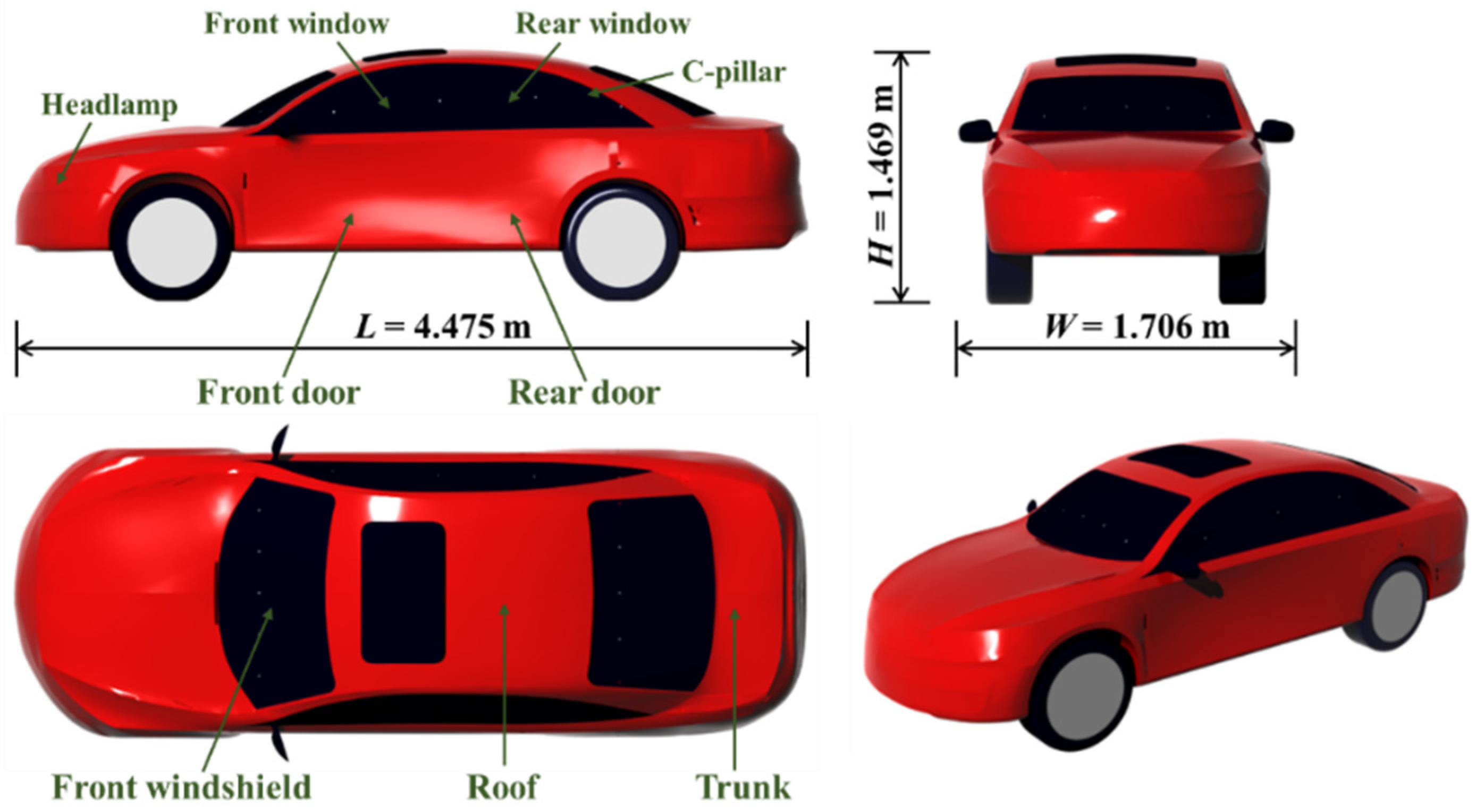
Figure 1. Simplified geometric model of the sedan.
Applsci 14 07522 g001
Figure 2. Geometric characteristics of the computational domain.
Applsci 14 07522 g002
Figure 3. Mesh model applied to the IDDES computational models (B1, B2 and B3 are the leading area, the fluid area adjacent to the sedan, and the trailing layup areas, respectively; C1 and C2 indicate the #1 encryption zone and #2 encryption zone, respectively).
Applsci 14 07522 g003
Figure 4. Mesh distribution around the sedan: (a) coarse; (b) medium; (c) fine.
Applsci 14 07522 g004
Figure 5. Comparison of the lateral force coefficients of the sedan in three turbulence modeling approaches: (a) RNG k-ε; (b) LES; (c) IDDES.
Applsci 14 07522 g005
Figure 6. Layout of the measurement points on the surface of the sedan and the shoulder of the road.
Applsci 14 07522 g006
Figure 7. Comparison between pressures and its averaged values measured by field tests and CFD methods.
Applsci 14 07522 g007
Figure 8. Comparison between the results at the 0.9 m height of the shoulder in the field test and the CFD numerical simulation: (a) wind speed; (b) pressure.
Applsci 14 07522 g008
Figure 9. Comparison of the sedan aerodynamic loads in the experiment and numerical predictions: (a) drag force coefficient; (b) lateral force coefficient.
Applsci 14 07522 g009
Figure 10. The temporal progression of the sedan’s aerodynamic loads and running posture as it transitions through the dune: (a) lateral force coefficient; (b) rolling moment coefficient; (c) yawing moment coefficient.
Applsci 14 07522 g010
Figure 11. The time history curves of the pressure at the measurement points predicted by the three turbulence modeling approaches: (a) windward side; (b) leeward side.
Applsci 14 07522 g011
Figure 12. Pressure distribution of the sedan surface at the t1 moment: (a) RNG k-ε; (b) LES; (c) IDDES (Subscripts 1, 2, 3, and 4 indicate the windward, leeward, top view, and bottom view of the sedan, respectively; the blue dashed line marks the main differences in pressure distribution in the results).
Applsci 14 07522 g012
Figure 13. Pressure distribution of the sedan surface at the t4 moment: (a) RNG k-ε; (b) LES; (c) IDDES (Subscripts 1, 2, 3, and 4 indicate the windward, leeward, top view, and bottom view of the sedan, respectively; the blue dashed line marks the main differences in pressure distribution in the results).
Applsci 14 07522 g013
Figure 14. Diagrams of the flow field at three representative cross-sections of the sedan as forecasted by the three turbulence modeling approaches at the moment t1: (a) RNG k-ε; (b) LES; (c) IDDES (Subscripts 1, 2, and 3 denote the cross-sections at the front wheels, the middle of the sedan, and the rear wheels, respectively).
Applsci 14 07522 g014
Figure 15. Diagrams of the flow field at three representative cross-sections of the sedan as forecasted by the three turbulence modeling approaches at the moment t4: (a) RNG k-ε; (b) LES; (c) IDDES (Subscripts 1, 2, and 3 denote the cross-sections at the front wheels, the middle of the sedan, and the rear wheels, respectively; the red dashed lines mark the main differences in vortex structure in the results).
Applsci 14 07522 g015
Figure 16. Evolution of the vortex structure around the sedan predicted by three turbulence modeling approaches before the sedan drives into the dune: (a) RNG k-ε; (b) LES; (c) IDDES (The blue dashed line marks the evolution of the vortex structure).
Applsci 14 07522 g016
Figure 17. Evolution of the vortex structure around the sedan predicted by three turbulence modeling approaches after the sedan drives into the dune: (a) RNG k-ε; (b) LES; (c) IDDES (The blue dashed line marks the evolution of the vortex structure).
Applsci 14 07522 g017
Figure 18. The temporal progression of the sedan’s aerodynamic loads under crosswinds and crosswind–sands: (a) lateral force coefficient; (b) rolling moment coefficient; (c) yawing moment coefficient.
Applsci 14 07522 g018aApplsci 14 07522 g018b
Table 1. Main parameters for calculation of the cases.
CaseTurbulence Modeling ApproachesThe Condition of the Flow FieldThe Speed of the Crosswind (m/s)The Driving Speed of the Sedan (m/s)Calculation Time (h)
1RNG k-εCrosswind2027.78127
2LESCrosswind2027.78203
3IDDESCrosswind2027.78141
4IDDESCrosswind–sand2027.78165
Table 2. The peak value and the corresponding amplitudes of the sedan’s aerodynamic load coefficients predicted by the three turbulence modeling approaches during the sedan driving within the dune.
Turbulence Modeling ApproachesAerodynamic ForceCzCmxCmy
RNG k-εMax0.604−0.0200.607
Min0.218−0.1040.323
Amplitude0.3860.0840.284
LESMax0.665−0.0480.744
Min0.212−0.1510.407
Amplitude0.4530.1030.337
IDDESMax0.705−0.0350.612
Min0.323−0.1270.247
Amplitude0.3820.0920.365
Table 3. Peak value and the corresponding amplitudes of the sedan’s three aerodynamic load coefficients under crosswind and crosswind–sands.
Types of the Incoming Flows Aerodynamic ForceCzCmxCmy
WindMax0.705−0.0350.612
Min0.323−0.1270.247
Amplitude0.3820.0920.365
Wind–sandMax0.671−0.0240.610
Min0.257−0.1150.297
Amplitude0.4140.0910.313
Disclaimer/Publisher’s Note: The statements, opinions and data contained in all publications are solely those of the individual author(s) and contributor(s) and not of MDPI and/or the editor(s). MDPI and/or the editor(s) disclaim responsibility for any injury to people or property resulting from any ideas, methods, instructions or products referred to in the content.