D*-KDDPG: An Improved DDPG Path-Planning Algorithm Integrating Kinematic Analysis and the D* Algorithm

Abstract

To address the limitations of the Deep Deterministic Policy Gradient (DDPG) in robot path planning, we propose an improved DDPG method that integrates kinematic analysis and D* algorithm, termed D*-KDDPG. Firstly, the current work promotes the reward function of DDPG to account for the robot’s kinematic characteristics and environment perception ability. Secondly, informed by the global path information provided by the D* algorithm, DDPG successfully avoids getting trapped in local optima within complex environments. Finally, a comprehensive set of simulation experiments is carried out to investigate the effectiveness of D*-KDDPG within various environments. Simulation results indicate that D*-KDDPG completes strategy learning within only 26.7% of the training steps required by the original DDPG, retrieving enhanced navigation performance and promoting safety. D*-KDDPG outperforms D*-DWA with better obstacle avoidance performance in dynamic environments. Despite a 1.8% longer path, D*-KDDPG reduces navigation time by 16.2%, increases safety distance by 72.1%, and produces smoother paths.

1. Introduction

In complex and dynamic environments, wheeled robots require real-time, efficient navigation to adapt to varying terrains and diverse obstacles, for which deep reinforcement learning methods offer new solutions to promote navigation efficiency [1]. Such methods continuously learn strategies to avoid obstacles through dynamic interactions between the robot and its environment. The Deep Deterministic Policy Gradient (DDPG) algorithm is a typical deep reinforcement learning algorithm that shows significant potential in small-scale path planning and dynamic obstacle avoidance in highly complex environments. However, the traditional DDPG shows two main limitations within the context of robot navigation: firstly, DDPG does not consider the kinematic characteristics of wheeled robots and might produce inefficient planning [2]; secondly, DDPG is prone to be trapped in local optima [3], due to the lack of global information in a complex environment.

This paper proposes the D*-KDDPG algorithm, an improved version of DDPG. It introduces two key enhancements: first, an upgraded reward function that considers the kinematic analysis of wheeled robots, thereby improving the model’s training efficiency and motion strategy optimization. Second, integrating the D* algorithm, which provides global map information as a guide, significantly enhances navigation efficiency and path quality by eliminating local optima in large-scale environments. Last, the paper thoroughly investigates the D*-KDDPG’s effectiveness under various map setups and scenarios, providing solid evidence of its potential in real-world applications.

The organization of this paper is as follows: Section 2 presents an overview of the research background and related work. Section 3 introduces the D*-KDDPG method, including the principle of DDPG, the robot kinematic analysis, the update of the reward function, and the integration of the D* algorithm. Section 4 validates D*-KDDPG’s effectiveness in the Gazebo environment. Section 5 summarizes the key findings of this research and proposes future directions.

2. Relate Work

Traditional path-planning algorithms fall into two categories: global path planning and local path planning [4]. Global planning algorithms, such as Dijkstra, D*, A*, Rapidly-exploring Random Tree (RRT), and Genetic Algorithms (GA), can perform well in static environments but are inefficient when dealing with dynamic obstacles. In contrast, local path planning algorithms, such as Artificial Potential Field (APF), Dynamic Window Approach (DWA), and Ant Colony Optimization (ACO), can avoid obstacles in real-time with smooth paths but show restricted robustness and generality due to unpractical parameters. Researchers have tried to address the abovementioned issues from two perspectives.

The first approach optimizes and combines traditional methods. Wang et al. reduced the overall road cost for mobile robots by introducing road condition indicators into the evaluation function of the A* algorithm [5]. The A* algorithm has been combined with the Dynamic Window Approach (DWA) to enhance the dynamic obstacle avoidance capability of robots in complex environments [6,7]. Wang et al. optimized the DWA algorithm by introducing differential manifold tangent vectors and improving the evaluation function, enhancing the rationality and smoothness of path planning in environments with dense obstacles [8]. However, these improved methods still suffer from poor adaptability and reliance on initial parameter values in dynamic environments.

The second approach adopts reinforcement learning for path planning. The Q-learning algorithm is a widely used classic reinforcement learning algorithm [9], thanks to its simplicity and quick converging speed. However, it suffers from the “curse of dimensionality” when dealing with complex environments. Deep reinforcement learning (DRL) combines deep learning with reinforcement learning, leveraging deep learning’s capability to handle high-dimensional information to learn end-to-end strategies for complicated planning tasks. However, DRL-based path planning methods, such as DQN [10], double DQN [11], and dueling DQN [12], require transforming high-dimensional continuous actions into discrete action sequences, which may alter the structure of the action domain and hinder the completion of path planning tasks. Lillicrap et al. proposed the deep deterministic policy gradient (DDPG) algorithm [3], which combines both DQN and deterministic policy gradient (DPG) [13]. In the same report, the DDPG was validated with improved stability and reduced time compared to DQN.

Despite its high stability and efficiency, DDPG fails to obtain an optimal motion strategy due to its reward function’s lack of kinematic characteristics. The absence leads to redundant actions, slow responses to obstacles, and growing collision risk. Moreover, the algorithm gets trapped in local optima in complex environments, due to the lack of global information. To address these issues, Deng et al. set multiple optimization objectives based on the longitudinal kinematic characteristics of vehicles to improve vehicles’ following performance [14]. Yan et al. optimized the DDPG reward function based on robot kinematics, effectively overcoming DDPG’s drawbacks, like long training cycles and poor path planning quality [2]. Zhu et al. designed a new DDPG reward function based on vehicle kinematics and established an RDL-based speed control model. The presented model significantly improves autonomous driving safety, operational efficiency, and comfort [15]. On the other hand, to address the ‘trapped in local optima’ issue, Li et al. addressed the ‘trapped in local optima’ issue of the RL planner via local RDL-based hierarchical planning [16]. Chen et al. introduced Sequential Linear Programming (SLP) as global guidance to improve DDPG, remarkably increasing the ratio of successful navigations in dynamic environments [17].

In summary, integrating kinematic characteristics into DDPG can optimize a robot’s path planning with a smoother path, while utilizing global information can enhance DDPG’s navigation efficiency and adaptability. Therefore, this paper proposes a D*-KDDPG model that integrates kinematic characteristics with global information into DDPG to improve robot motion strategy.

3. Methods

3.1. DDPG Introduction

DDPG is a reinforcement learning algorithm that combines Q-learning and policy gradient methods. The network structure of DDPG is shown in Figure 1, including an online actor–network and an online critic network to learn optimal strategies. The online actor–network interacts with the external environment in real time, during which it takes actions under the online critic network’s guidance. The online critic network supervises the online actor–network to conduct impending actions based on historical experience while continuously updating its own value function Q. Notably, DDPG follows DQN’s idea and introduces a replay buffer and two target networks to guarantee training stability. The replay buffer caches historical experiences in the form of (s_i, a_i, r_i, s_i+1) for the critic network to reference. The target networks save strategies learned by two online networks in recent training epochs, with which they stabilize the critic’s evaluation and actor’s learning.

During each training epoch, DDPG randomly samples a batch of historical experiences from the replay buffer to form a learning sample set N*. For each sample (s_i, a_i, r_i, s_i+1) in N*, DDPG calculates the target value y_i [3],

$$y_i=r_i+\gamma {\mathrm{Q}}^{\prime }(s_{i+1},{\mu }^{\prime }(s_{i+1}|{\theta }^{{\mu }^{\prime }})|{\theta }^{Q^{\prime }})$$

(1)

where r_i represents the immediate reward, γ is the discount factor, the target actor–network µ’(s_i+1|θ^µ’) is estimated by its parameter θ^µ’, and Q’ is the evaluation reference provided by the target critic network and its parameter θ^Q’ based on temporal difference method. Correspondingly, the online critic network calculates the loss L with target value y_i [3], such as,

$$L={\displaystyle \frac{1}{N}}{\displaystyle {\sum }_i}{(y_i-Q(s_i,a_i|{\theta }^Q))}^2$$

(2)

where N is the number of experience samples, Q(s_i, a_i|θ^Q) represents the evaluation made by the online critic network based on current state s_i and action a_i. Meanwhile, the online critic network updates its parameters θ^Q to minimize the loss L. With this updated value function Q, the online critic network guides the online actor to update its strategy θ^µ [3], such as,

$$\nabla {\theta }^{\mathsf{\mu }}J\approx {\displaystyle \frac{1}{N}}{\displaystyle {\sum }_i}{\nabla }_{a}Q(s,a|{\theta }^Q){|}_{s=si,a=\mu (si)}\nabla {\theta }^{\mathsf{\mu }} \mu (\mathrm{s}|{\theta }^{\mu })|s_i$$

(3)

At the end of every training epoch, DDPG uses a ‘soft update’ to update the weights of two target networks [3], which helps the target network track the online networks’ progress and maintain learning stability, such as,

$$\begin{array}{l}{\theta }^{\mathsf{\mu }\prime }\leftarrow \tau {\theta }^{\mathsf{\mu }}+(1-\tau ){\theta }^{\mathsf{\mu }\prime }\\ {\theta }^{\mathrm{Q}\prime }\leftarrow \tau {\theta }^Q+(1-\tau ){\theta }^{\mathrm{Q}\prime }\end{array}$$

(4)

Once the training is completed, the online actor determines the next action a based on its current state s, strategy θ^µ, and real-time interactions with the environment [3], such as,

$$a=\mu (s|{\theta }^{\mu })+N$$

(5)

where the random noise N is added by the actor–network to extend the exploration range.

As shown in Equation (1), the reward function r directly influences the target value y_i during training, consequently altering the loss value L and the update of value function Q. Thus, r reflects DDPG’s preference in strategy learning, and a qualified r, as the critic’s feedback to the actor’s learning, can help the critic network guide the actor to learn the expected strategy more effectively.

3.2. KDDPG: Local Path Planning Method Based on Kinematic Analysis

When applied to robot path planning, DDPG should decide its next action based on the robot’s current state and environmental information (such as the goal position and obstacle positions). Specifically, DDPG should regard a robot’s kinematic characteristics, its proximity to the goal, and its surrounding environment to ensure effective path planning. Therefore, this work will present a two-wheel robot’s kinematic model and its environment perception model in Section 3.2.1 and then introduce how to integrate them into robot path planning via updating DDPG’s reward function in Section 3.2.2.

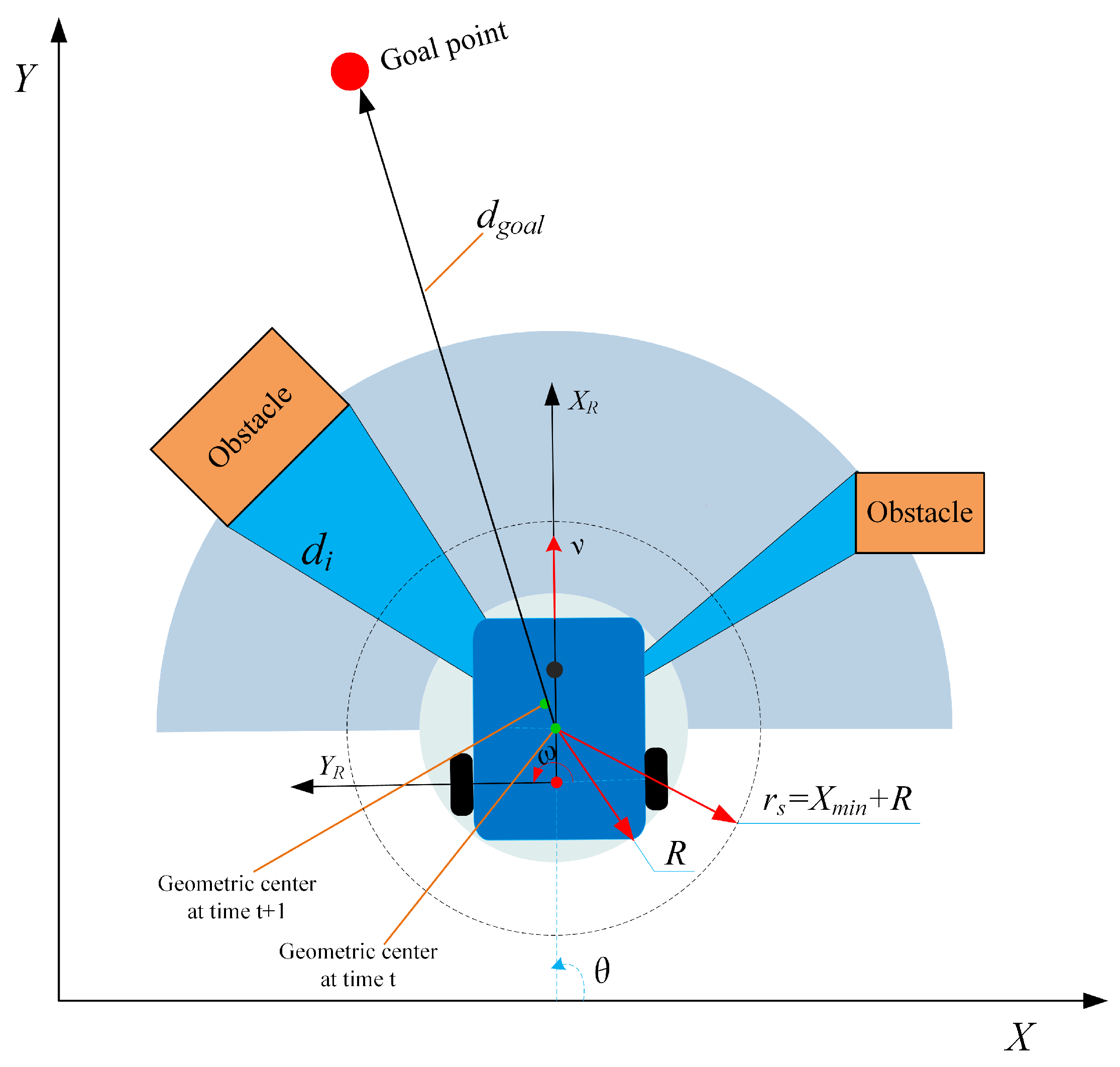
3.2.1. Kinematic Model and Environmental Perception Model

The kinematic model and the environmental perception model of a two-wheeled differential mobile robot are shown in Figure 2, illustrating the robot’s position and state at consecutive time points as well as the surrounding environmental information. The robot’s state update equation based on its kinematic is:

$$s_{t+1}=f(s_t,\overrightarrow{a_t})+\overrightarrow{{\delta }_t}=\left[\begin{array}{c}{x}_t+vT\cos ({\theta }_t+{\displaystyle \frac{\omega T}{2}})+{\delta }_{x,t}\\ y_t+vT\sin ({\theta }_t+{\displaystyle \frac{\omega T}{2}})+{\delta }_{y,t}\\ {\theta }_t+\omega T+{\delta }_{\theta ,t}\end{array}\right]$$

(6)

where T is the unit sampling period, state s_t = [x_t, y_t, θ_t]^T collectively represents the robot’s position (x_t, y_t) and orientation angle θ_t, and control variables a_t = [v, ω]^T updates robot’s state via its linear velocity v and angular velocity ω, δ_x,t, δ_y,t, and δ_θ,t denotes Gaussian noises in x, y, and θ, respectively, simulating the impact of real-world uncertainties on the robot’s motion.

For a robot running at speed v, the corresponding minimum braking distance X_v,min is given by:

$$X_{v,min}={\displaystyle \frac{v^2}{2a_{max}}}$$

(7)

where a_max is the robot’s maximum braking deceleration. Obviously, a higher running speed results in a longer minimum braking distance. Thus, the current work denotes the robot’s minimum braking distance at its maximum speed v_max as the buffer distance X_min, and defines the robot’s safety radius r_s accordingly, such as,

$$\begin{array}{l}{r}_s=X_{min}+R\\ X_{min}={\displaystyle \frac{v_{max}^2}{2a_{max}}}\end{array}$$

(8)

where R is the robot’s minimum bounding radius. Furthermore, by comparing r_s with the distance between the robot and the obstacle, we can determine whether the robot is in a collision zone.

For environmental perception, we set the goal attractive potential field U_goal(s_t) and the obstacle repulsive potential field U_obs(s_t) as:

$$\begin{array}{l}{U}_{goal}(s_t)={\displaystyle \frac{1}{2}}k{d_{goal}}^2\\ U_{obs}(s_t)={\displaystyle \sum _{i=1}^n{e}_i}\cdot (d_i-r_s)\end{array}$$

(9)

where k is the coefficient of the attractive potential field, d_goal is the distance between the robot’s current position and the goal point, d_i is the scanning distance of the i-th laser beam, and e_i is the weight of d_i. With such notions, d_i − r_s represents the difference between the obstacle’s distance and the safety distance, and a smaller (d_i − r_s) indicates a higher collision risk. The size of the obstacle is measured by the number of laser beams that sense the obstacle. U_goal(s_t) indicates the robot’s proximity to the goal point, while U_obs(s_t) comprehensively considers the distance, relative direction, and size of the obstacle, indicating the robot’s proximity to the obstacle. We then refer to the gradients of U_goal(s_t) and U_obs(s_t) as,

$$\begin{array}{l}{F}_{goal,t}=-\nabla U_{goal}(s_t)\\ F_{obs,t}=\nabla U_{obs}(s_t)\end{array}$$

(10)

where F_goal,t represents a vector pointing towards the goal, and F_goal,t represents a vector pointing away from the obstacles. Therefore, F_goal,t directs the robot to move towards the goal, and F_goal,t guides the robot to move away from obstacles.

Based on the above two models, we will design a reward function to optimize the robot’s path-planning performance in the following section.

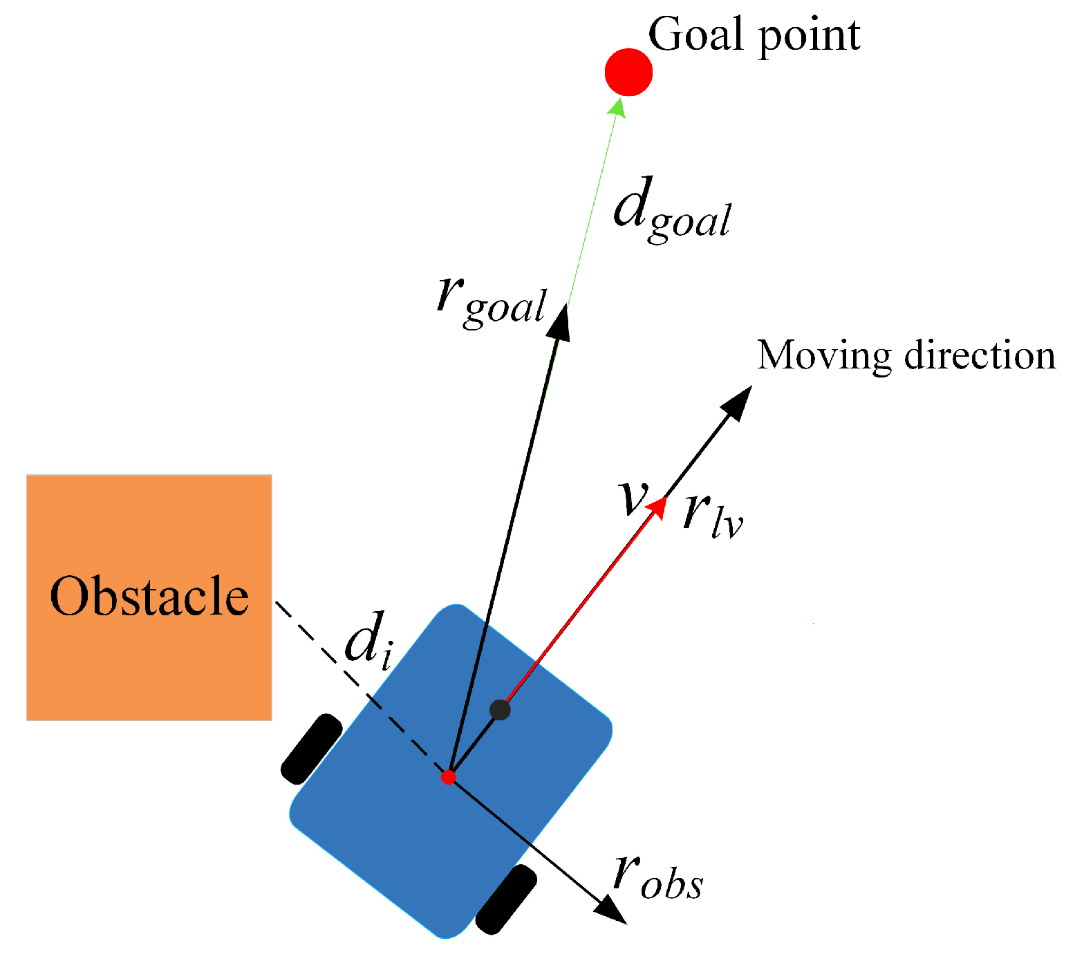
3.2.2. Reward Function Setup

Combining the kinematic model and environmental perception of the robot in Section 3.2.1, this paper upgrades DDPG’s reward function r as follows; its composition is shown in Figure 3.

$$r={\omega }_{goal}\cdot r_{goal}+{\omega }_{obs}\cdot r_{obs}+{\omega }_{smooth}\cdot r_{smooth}+{\omega }_{lv}\cdot {r_l}_v$$

(11)

where r_goal, r_obs, r_smooth, and r_lv denote reward consideration on the robot’s goal approach, obstacle avoidance, path smoothness, and navigation efficiency, respectively, and ω_goal, ω_obs, ω_smooth, and ω_lv are the corresponding weights.

Reward r_goal is defined based on F_goal,t (Equation (10)), such as,

$$r_{goal}=\{\begin{array}{l}{r}_{\mathrm{arrival} } \mathrm{if} d_{goal}<d_{gmin}\\ F_{goal,t} otherwise\end{array}$$

(12)

where d_goal is the distance from the robot to the goal, and d_gmin is the distance threshold. When d_goal is less than d_gmin, a significant positive reward r_arrival is provided.

Rewards r_obs are defined based on F_obs,t (Equation (10)), such as,

$$r_{obs}=\{\begin{array}{l} r_{collision} \mathrm{if} d_{ro}<d_{collision}\\ F_{obs,t} otherwise\end{array}$$

(13)

where d_collision is the collision threshold determined by the robot’s actual dimensions. A collision occurs if the minimum scanning distance d_ro is less than d_collision, for which r_obs retrieves a significant negative reward r_collision.

Reward r_smooth encourages the robot to pursue a smooth path, avoiding excessive sharp turns. It denotes the changes in the robot’s linear velocity Δv and angular velocity Δω, such as,

$$r_{smooth}=- (\alpha \cdot \left|\Delta v\right|+\beta \cdot \left|\Delta \omega \right|)$$

(14)

where α and β are weight factors that balance the influence of changes in linear and angular velocities, respectively. This reward penalizes significant velocity changes and hence rewards smoother paths.

Reward r_lv encourages the robot to maintain a stable speed, thereby improving navigation efficiency, such as,

$${r_l}_v=\{\begin{array}{l}{r}_{lp} \mathrm{if} l_v<l_{vmin} \\ 0 otherwise\end{array}$$

(15)

where l_vmin is a predefined speed threshold. DDPG will receive a negative reward r_lp when the linear velocity v is smaller than l_vmin.

3.3. Integration of Global Algorithm D* with KDDPG

In large-scale dynamic environments, the DDPG model is limited by its perception range and lacks the utilization of global information, which can lead to redundant actions and getting trapped in local optima. This paper integrates a global path-planning algorithm named D* algorithm with KDDPG to enhance navigation efficiency and safety. The D*-KDDPG algorithm represents a typical two-layer path planning structure that integrates global and local path planning. The global path planner uses the D* algorithm to make high-level path decisions based on a known map, providing long-term goals and a route framework for the local path planner. Guided by the global path, the local path planner KDDPG refines and adjusts the path in real-time, responding quickly to environmental changes and avoiding unexpected obstacles. This two-layer structure combines the efficiency of global planning with the flexibility of local planning, enabling the path planning process to adapt to complex environmental changes while maintaining the pursuit of the overall goal. The pseudo-code for this integration is presented in Algorithm 1.

Algorithm 1 D*-KDDPG path-planning algorithm

Input: Map: 2D Grid Map, S: Start position, G: Goal position, S’(x, y): Current robot coordinates,    dgoal: The distance of robot to goal, ε: Reference-Goal threshold, δ: Goal-Reach threshold, KDDPG_Move:Pre-trained KDDPG model, MAXTIME: Timeout threshold. Output: Path to the Goal position 1: function D*-KDDPG (Map, S, G, S’(x, y), dgoal, ε, δ, KDDPG_Move, MAXTIME) 2:   Global Path ← D_star(Map, S, G) 3:   StartTime ← GetCurrentTime() 4:   for G’ in Global Path do 5:      while dgoal > δ do 6:         $\mathrm{Compare} \sqrt{{(x-G^{\prime }.x)}^2+{(y-G^{\prime }.y)}^2}$ with ε 7:         ReferenceGoal ← Select the point closest to threshold ε 8:         KDDPG_Move (S’, ReferenceGoal) 9:        TimeElapsed ← CurrentTime–StartTime 10:        if TimeElapsed > MAXTIME or Collision then 11:            return Fail to reach Goal 12:         end if 13:       end while 14:       if dgoal <= δ then 15:         return Success to reach Goal 16:       end if 17:    end for 18: end function

Algorithm 1 presents three stages of the D*-KDDPG algorithm. Firstly, the D* algorithm generates a global path based on a known 2D map. The generated path composes a sequence of path nodes connecting the robot’s initial position and the global goal. Next, for each stage of local path planning, D*-KDDPG selects a path node from the global path as a local reference goal. The path nodes are selected as candidates if their distances to the robot’s current locations are smaller than a given threshold ε, and the nearest one is selected as the local reference goal, accordingly. The global goal becomes the current reference goal if no candidate arises. Finally, KDDPG drives the robot toward the selected reference goal and completes the local path planning. The process continues until the robot achieves the global by following the global path generated by D*.

4. Experiments and Results

4.1. Training Experiment Setup

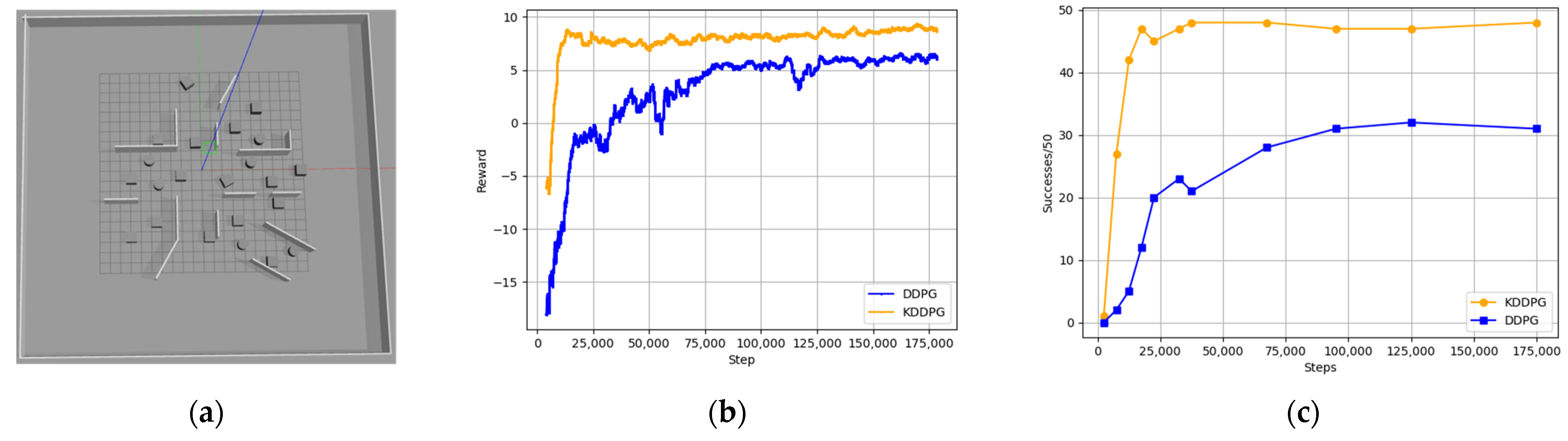
The current work employs Gazebo as the simulation environment for training and validation, within which a robot, “Turtlebot3 Waffle”, is selected as the experimental robot. The selected robot is equipped with encoders, an inertial measurement unit, and a laser radar, for which the parameters are shown in

Table 1. Main parameters of mobile robot.

Parameter	Value
Robot size (mm)	306 × 282.57 × 142.35
Max angle speed (rad/s)	1.82
Max speed (m/s)	0.26
Max payload (kg)	30

. The laser radar provides 24 equally angular spaced scan data, which cover an angular range of (−90°, 90°) and a distance range of (0.12 m, 3.0 m). In this study, the authors successfully implemented the proposed algorithm by coding. Furthermore, the improved DDPG and D* algorithms were integrated using the move_base package in the Robot Operating System (ROS). The training was conducted on a platform equipped with an NVIDIA GTX 2080Ti, using the Adam optimizer with a learning rate set to 0.0001.

4.2. Model Training

Figure 4 illustrates the model’s training performance. Against the simulation environment (Figure 4a), Figure 4b shows the changes in reward values during KDDPG and DDPG’s training, where the reward values are sampled every 4000 steps to minimize the random variations. Towards the same goal point, both KDDPG and DDPG are trained 50 times to count their success rate (Figure 4c).

The results demonstrate that KDDPG outperforms DDPG in terms of convergence speed and navigation performance. KDDPG converges at a success rate of 90% after approximately 20,000 steps, while DDPG achieves a 60% success rate after 75,000 steps, resulting in a four-fold longer training time.

4.3. Experiments

The trained DDPG, KDDPG, and D*-KDDPG models are further compared with D*-DWA to benchmark their performance, where D*-DWA and D*-KDDPG rely on a global map for navigation, and DDPG and KDDPG perform mapless navigation. The following metrics were used for the performance comparison:

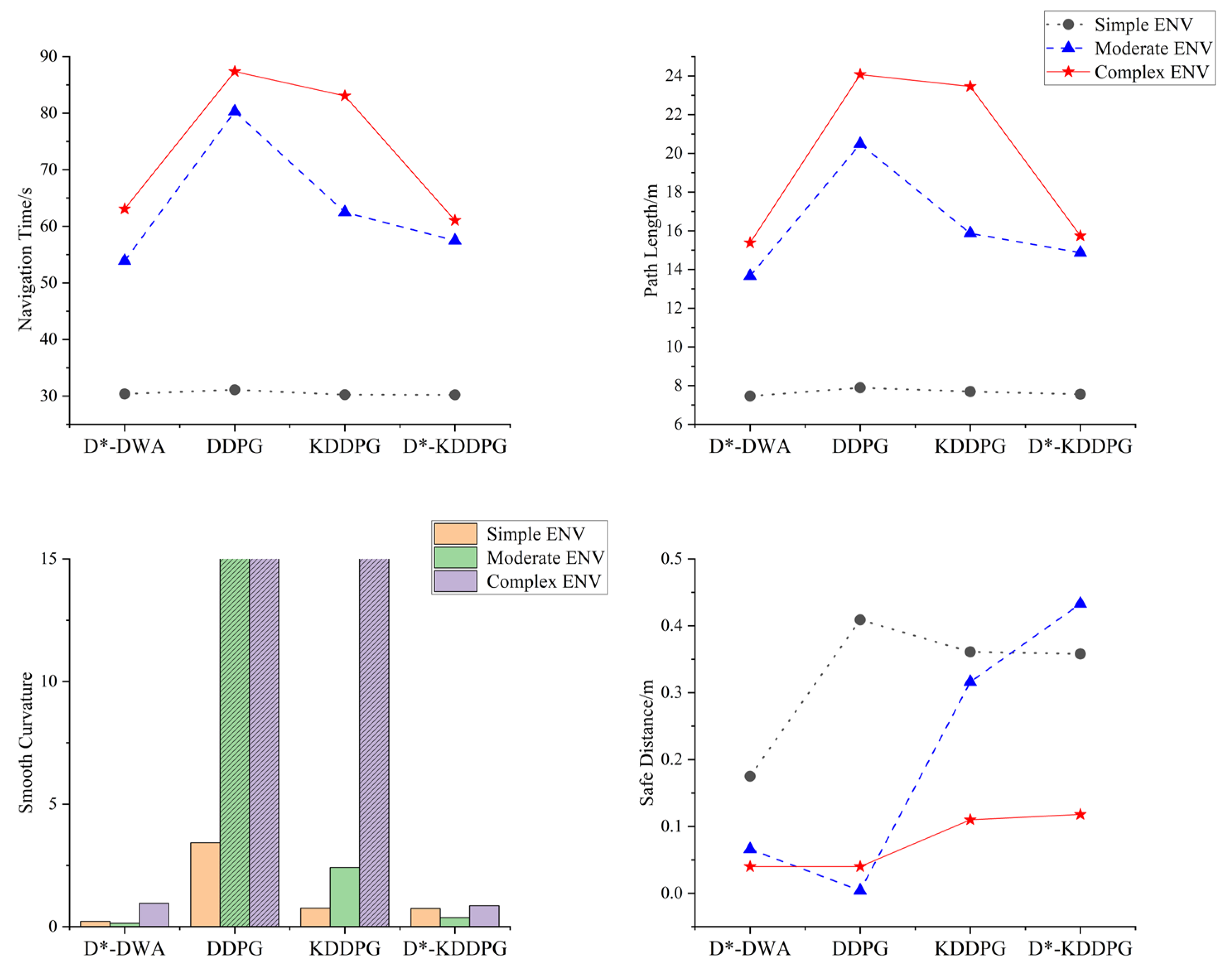
• Navigation Time (NT): The time required to complete the navigation.
• Path Length (PL): The total length of the generated path.
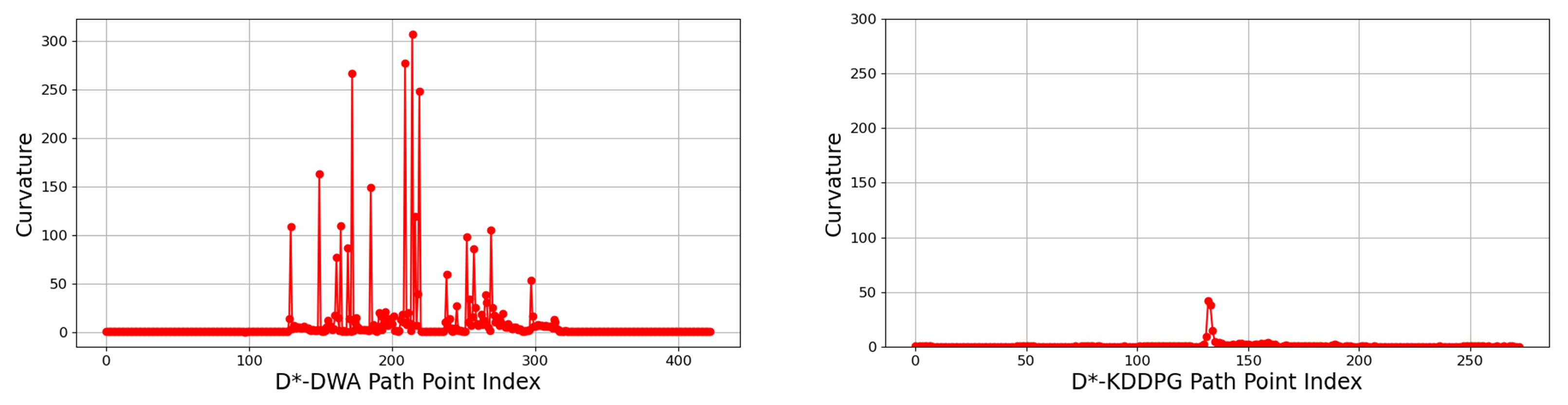
• Curvature Smoothness (CS): The integral of the square of the curvature, which is used to measure the smoothness of the path [18]; lower values indicate smoother paths.
• Safety Distance (SD): A distance used for collision detection, which is calculated by subtracting 0.141 m (a reference value based on the robot’s dimensions) from the radar’s detection distance. A collision is assumed to happen when SD reaches zero.

In particular, when a collision occurs, the path planning fails, and NT is set to the timeout MAXTIME as specified in Section 3.3. It is noteworthy that a larger safety distance can enhance the safety of the planned path but may increase navigation time and path length.

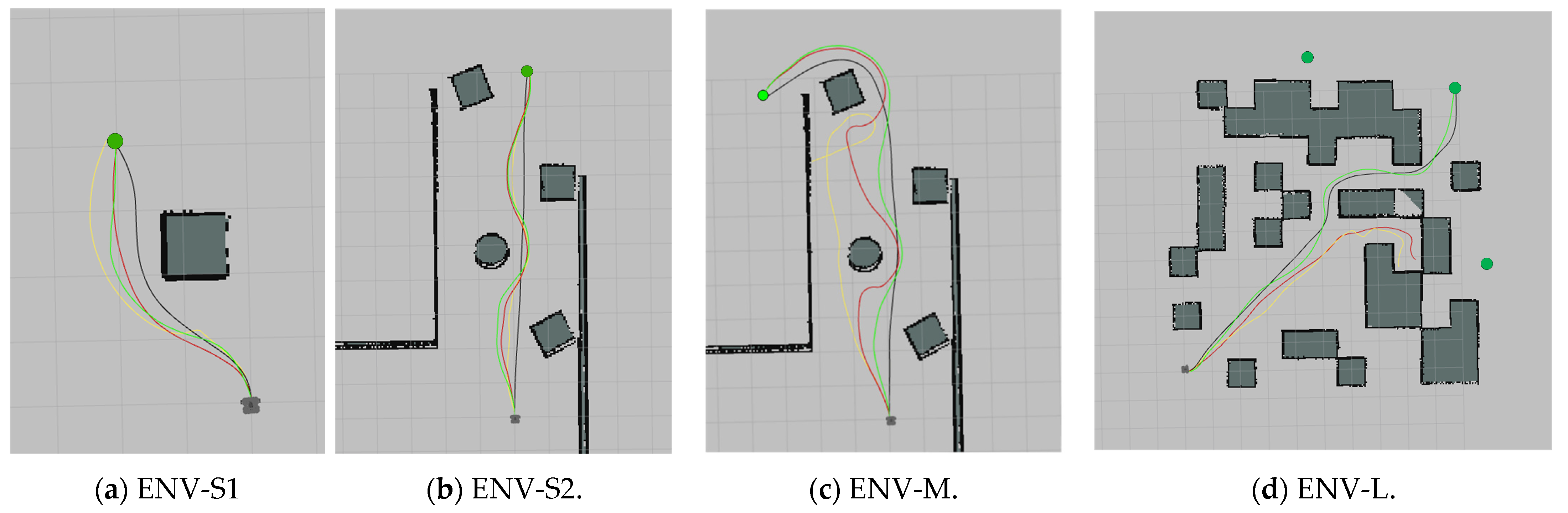
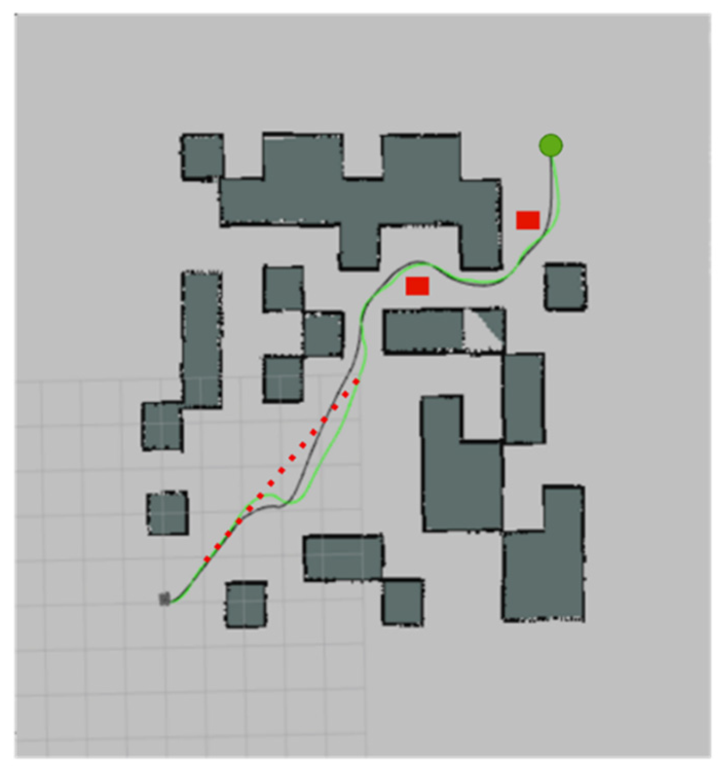
4.3.1. Static Environment Experiments

Four static environments are constructed to compare the four algorithms’ performance. The four environments, namely ENV-S1, ENV-S2, ENV-M, and ENV-L, feature varying complexities, i.e., ENV-S1 and EVN-S2 are relatively simple, ENV-M features a medium-level complexity, and ENV-L is the most complex with three alternative targets. The path results and experimental data are shown in Figure 5 and Figure 6, respectively. Notably, DDPG produces collisions in ENV-M and ENV-L, and KDDPG produces a collision in ENV-L, for which the corresponding curvature smoothness is set to the maximum and illustrated in shadows in Figure 6.

As shown in Figure 6, regarding path planning efficiency, KDDPG outperforms DDPG with a 9.9% smaller NT and a 9.2% shorter PL. However, KDDPG performs several unnecessary actions and shows limited improvement in the complex ENV-L because it fails to utilize the environment’s global information. In contrast, D*-KDDPG achieves an 11.5% less NT and a 13.6% shorter PL than KDDPG by consulting the global information, and the same model results in a 0.8% more NT and a 3.9% longer PL than D*-DWA, another model utilizing the global information. For path smoothness, KDDPG’s performance is much better than DDPG but poorer than D*-KDDPG and D*-DWA, as the latter two produce equivalently low curvature smoothness. For robot safety, D*-KDDPG maintains a safety distance 67.3% larger than those of D*-DWA.

In summary, D*-KDDPG can plan shorter, smoother, and safer paths within reduced periods than DDPG and KDDPG, and it produces paths featuring significantly enhanced safety and approximately the same length and curvature smoothness as D*-DWA and D*-KDDPG without additional time costs.

4.3.2. Dynamic Environment Experiments

In the following experiments, an obstacle is placed dynamically in the robot’s impending path to test navigation algorithms’ ability to handle unexpected obstacles. The obstacle is a square with varying sizes (0.5 or 1.0 m) at varying distances (0.6, 1, and 1.5 m) from the running robot. The two sizes and three distances produce six experiment scenarios labeled (a) to (f), as shown in Figure 7. The experimental results are presented in Figure 8 and

Table 2. Curvature Smoothness of Dynamic Environment.

Algorithm	a	b	c	d	e	f
D*-DWA	4819	6546	17,661	1.71	190	2792
DDPG	collision	collision	collision	74	1.35	collision
KDDPG	20	2.79	collision	1.28	1.30	419
D*-KDDPG	2.61	1.03	137	0.666	0.519	11.9

.

DDPG can avoid small and distant obstacles (Figure 7d,e) but fails to avoid massive obstacles in near range. In contrast, KDDPG can avoid obstacles in most cases, and two global-information-aided algorithms, D*-KDDPG and D*-DWA, successfully avoid obstacles in all scenarios. For the latter two models, D*-DWA performs unnecessary actions in some cases because it fails to locate an avoidance obstacle in time, leading to sharp shifts in curvature and extended PL.

More specifically, per path planning efficiency, D*-KDDPG improves the average NT by 34.1%, 22.2%, and 16.2% than DDPG, KDDPG, and D*-DWA, respectively, featuring relatively minor variance (less than 3.98). On the other hand, the average PL produced by D*-KDDPG is approximately equal to that of D*-DWA, with an increase of 1.8%. As a comparison, D*-KDDPG outperforms DDPG and KDDPG significantly by a 24.2% shorter average PL and 15.9% less variable. Per path safety, D*-KDDPG and KDDPG maintain a high average SD, where D*-KDDPG shows a minor variance. D*-KDDPG improves SD by 72.1% compared to D*-DWA. Per path smoothness, D*-KDDPG shows significant improvements in curvature smoothness compared to other methods. D*-DWA exhibits large curvature changes when facing dynamic obstacles due to the high weight of movements in DWA’s evaluation function and the resulting sharp adjustments in speed. In contrast, D*-KDDPG effectively diminishes large curvature changes thanks to its long-term planning and continuous action space planning capabilities. Moreover, Figure 9 illustrates the curvature of paths planned by D*-DWA and D*-KDDPG in scenario (c) as a validation.

In the ENV-L, static and dynamic obstacles were added to compare D*-DWA and D*-KDDPG within such a complicated environment. Static obstacles of size 0.5 m × 0.4 m are placed at coordinates (6.5, 7) and (9.25, 8.5), respectively. Additionally, a cylindrical dynamic obstacle with a diameter of 1 m and a speed of 0.26 m/s is introduced along the route from (5, 5) to (1, 1). Figure 10 illustrates the resulting paths, with experimental data listed in

Table 3. Dynamic Complexity Environment Path data.

Algorithm	NT	PL	SC	SD
D*-DWA	64.622	16.145	9.512	0.042
D*-KDDPG	63.075	16.554	2.915	0.108

. The data indicates that D*-KDDPG shows improvements in the other three metrics compared to D*-DWA while maintaining a comparable PL.

In summary, compared to D*-DWA, D*-KDDPG reduces navigation time and improves navigation efficiency when facing dynamic obstacles. Additionally, it significantly enhances safety distance and curvature smoothness, demonstrating its superiority in obstacle avoidance safety and navigation efficiency.

5. Conclusions

The proposed D*-KDDPG method effectively improves DDPG by integrating kinematic analysis and the D* algorithm, significantly enhancing the model’s path planning quality and safety while avoiding local optima issues. The proposed method significantly improves path planning efficiency in training and experiments. Training experiments indicate that D*-KDDPG achieves convergence with only 26.7% of the training steps required by DDPG and a higher navigation success rate. For experiments, D*-KDDPG outperforms DDPG and KDDPG with a higher success rate, faster planning speed, and more secure paths for static and dynamic scenarios. In static scenarios, D*-KDDPG shows only a marginal increase in path length and navigation time (less than 3.98%) compared to D*-DWA while increasing the safety distance by 67.3%. Also, D*-KDDPG demonstrates higher navigation efficiency than D*-DWA in dynamic scenarios since it achieves a 16.2% reduction in navigation time, improved curvature smoothness, and a 72.1% increase in safety distance. Future research will focus on improving the robustness of the algorithm and the fusion of sensor data to optimize the robot’s path-planning performance.

References

1. Aradi, S. Survey of Deep Reinforcement Learning for Motion Planning of Autonomous Vehicles. IEEE Trans. Intell. Transport. Syst. 2022, 23, 740–759. [Google Scholar] [CrossRef]
2. Yan, C.; Chen, G.; Li, Y.; Sun, F.; Wu, Y. Immune Deep Reinforcement Learning-Based Path Planning for Mobile Robot in Unknown Environment. Appl. Soft Comput. 2023, 145, 110601. [Google Scholar] [CrossRef]
3. Lillicrap, T.P.; Hunt, J.J.; Pritzel, A.; Heess, N.; Erez, T.; Tassa, Y.; Silver, D.; Wierstra, D. Continuous Control with Deep Reinforcement Learning. arXiv 2015, arXiv:1509.02971 2015. [Google Scholar]
4. Zhang, H.; Lin, W.; Chen, A. Path Planning for the Mobile Robot: A Review. Symmetry 2018, 10, 450. [Google Scholar] [CrossRef]
5. Wang, X.; Zhang, H.; Liu, S.; Wang, J.; Wang, Y.; Shangguan, D. Path Planning of Scenic Spots Based on Improved A* Algorithm. Sci. Rep. 2022, 12, 1320. [Google Scholar] [CrossRef] [PubMed]
6. Jiang, C.; Zhu, H.; Xie, Y. Dynamic Obstacle Avoidance Research for Mobile Robots Incorporating Improved A-Star Algorithm and DWA Algorithm. In Proceedings of the 2023 3rd International Conference on Computer Science, Electronic Information Engineering and Intelligent Control Technology (CEI), Wuhan, China, 15–17 December 2023; pp. 896–900. [Google Scholar]
7. Guan, C.; Wang, S. Robot Dynamic Path Planning Based on Improved A* and DWA Algorithms. In Proceedings of the 2022 4th International Conference on Control and Robotics (ICCR), Guangzhou, China, 2 December 2022; pp. 1–6. [Google Scholar]
8. Wang, H.; Ma, X.; Dai, W.; Jin, W. Research on Obstacle Avoidance of Mobile Robot Based on Improved DWA Algorithm. Comput. Eng. Appl. 2023, 59, 326–332. [Google Scholar]
9. Watkins, C.J.C.H. Learning from Delayed Rewards. 1989. Available online: https://www.academia.edu/download/50360235/Learning_from_delayed_rewards_20161116-28282-v2pwvq.pdf (accessed on 25 July 2024).
10. Mnih, V.; Kavukcuoglu, K.; Silver, D.; Rusu, A.A.; Veness, J.; Bellemare, M.G.; Graves, A.; Riedmiller, M.; Fidjeland, A.K.; Ostrovski, G.; et al. Human-Level Control through Deep Reinforcement Learning. Nature 2015, 518, 529–533. [Google Scholar] [CrossRef] [PubMed]
11. Van Hasselt, H.; Guez, A.; Silver, D. Deep Reinforcement Learning with Double Q-Learning. In Proceedings of the AAAI Conference on Artificial Intelligence, Phoenix, AZ, USA, 12–17 February 2016; Volume 30. [Google Scholar]
12. Wang, Z.; Schaul, T.; Hessel, M.; Hasselt, H.; Lanctot, M.; Freitas, N. Dueling Network Architectures for Deep Reinforcement Learning. In Proceedings of the International Conference on Machine Learning, New York, NY, USA, 20–22 June 2016; pp. 1995–2003. [Google Scholar]
13. Silver, D.; Lever, G.; Heess, N.; Degris, T.; Wierstra, D.; Riedmiller, M. Deterministic Policy Gradient Algorithms. In Proceedings of the International Conference on Machine Learning, Beijing, China, 21–26 June 2014; pp. 387–395. [Google Scholar]
14. Deng, X.-H.; Hou, J.; Tan, G.-H.; Wan, B.-Y.; Cao, T.-T. Multi-Objective Vehicle Following Decision Algorithm Based on Reinforcement Learning. Kongzhi Yu Juece/Control Decis. 2021, 36, 2497–2503. [Google Scholar] [CrossRef]
15. Zhu, M.; Wang, Y.; Pu, Z.; Hu, J.; Wang, X.; Ke, R. Safe, Efficient, and Comfortable Velocity Control Based on Reinforcement Learning for Autonomous Driving. Transp. Res. Part C Emerg. Technol. 2020, 117, 102662. [Google Scholar] [CrossRef]
16. Li, H.; Luo, B.; Song, W.; Yang, C. Predictive Hierarchical Reinforcement Learning for Path-Efficient Mapless Navigation with Moving Target. Neural Netw. 2023, 165, 677–688. [Google Scholar] [CrossRef] [PubMed]
17. Chen, Y.; Liang, L. SLP-Improved DDPG Path-Planning Algorithm for Mobile Robot in Large-Scale Dynamic Environment. Sensors 2023, 23, 3521. [Google Scholar] [CrossRef] [PubMed]
18. Horn, B.K. The Curve of Least Energy. ACM Trans. Math. Softw. (TOMS) 1983, 9, 441–460. [Google Scholar] [CrossRef]
Figure 1. DDPG framework.
Applsci 14 07555 g001
Figure 2. The kinematic model and the environmental perception model of a two-wheel mobile robot.
Applsci 14 07555 g002
Figure 3. KDDPG Reward Function.
Applsci 14 07555 g003
Figure 4. Training performance comparison: (a) the Gazebo simulation environment; (b) reward comparison; (c) success rate comparison.
Applsci 14 07555 g004
Figure 5. Performance comparison of four algorithms in different static environments. The green dots represent target points. The black lines indicate the D*-DWA paths, the yellow lines indicate the DDPG paths, the red lines indicate the KDDPG paths, and the green lines indicate the D*-KDDPG paths.
Applsci 14 07555 g005
Figure 6. Path date of four algorithms in different static environments.
Applsci 14 07555 g006
Figure 7. Performance comparison of four algorithms in different dynamic environments is depicted in subfigures (af), where each subfigure represents a unique setup with varying dimensions and distances of dynamic obstacles. The green dots represent target points, and the red squares represent dynamic obstacles. The black lines indicate the D*-DWA paths, the yellow lines indicate the DDPG paths, the red lines indicate the KDDPG paths, and the green lines indicate the D*-KDDPG paths.
Applsci 14 07555 g007
Figure 8. Dynamic Environment Path data.
Applsci 14 07555 g008
Figure 9. D*-DWA and D*-KDDPG Path Curvature.
Applsci 14 07555 g009
Figure 10. D*-DWA and D*-KDDPG algorithms performance in dynamic complexity environments. The green dot represent target point, and the red squares represent dynamic obstacles, and the red dash line represents the path of a cylindrical obstacle (1 m diameter, 0.26 m/s speed) from (5, 5) to (1, 1). The black lines indicate the D*-DWA paths, and the green lines indicate the D*-KDDPG paths.
Applsci 14 07555 g010