
Investigating Blind Spot Design Effects on Drivers’ Cognitive Load with Lane Changing: A Comparative Experiment with Multiple Types of Intelligent Vehicles

Abstract
1. Introduction
2. Methodology
2.1. Experiments
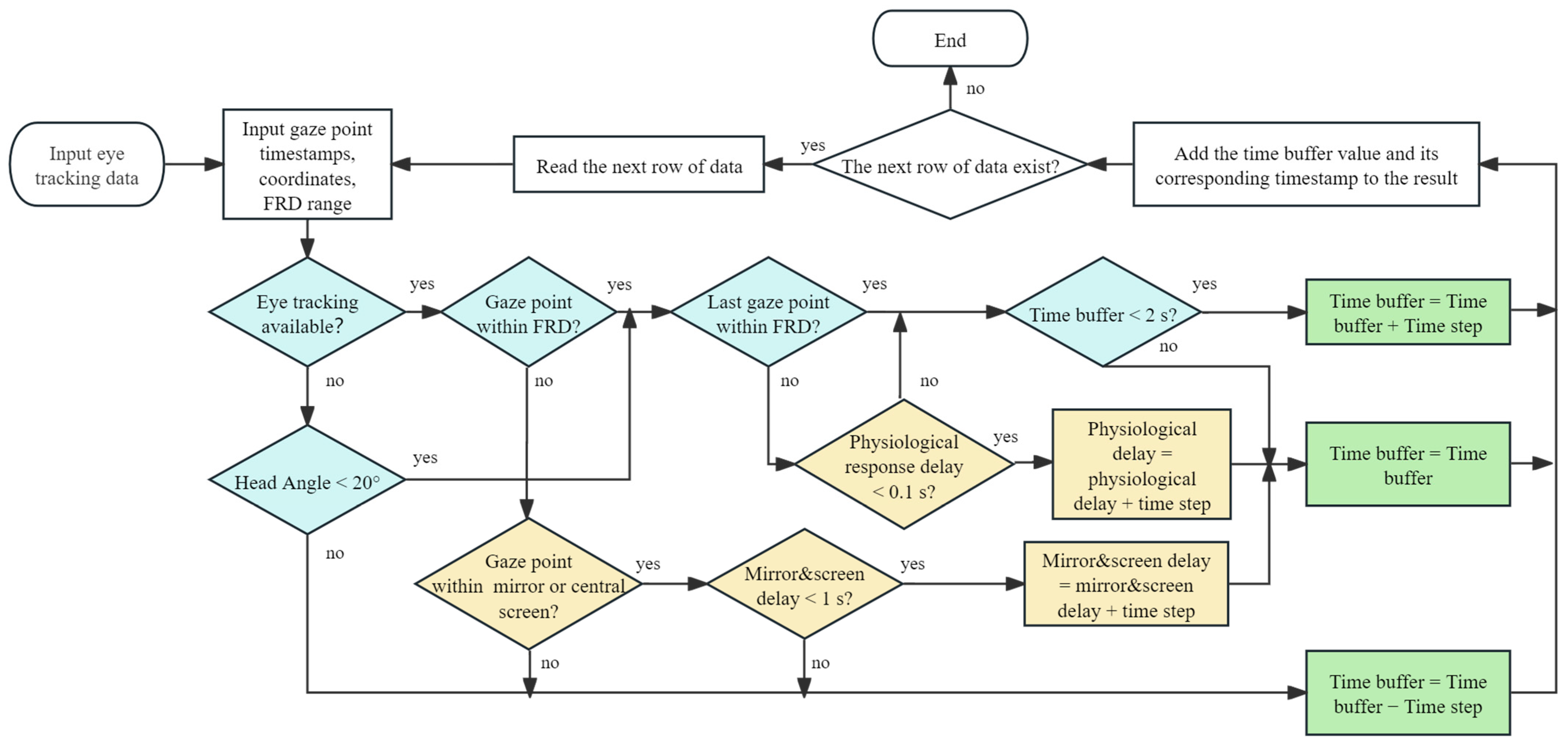
2.2. Algorithm for Cognitive Load Calculation
2.3. Impact Analysis Model
2.3.1. Kruskal–Wallis Test
2.3.2. Bayesian Logistic Ordinal Regression
2.3.3. Categorical Boosting
3. Data Collection
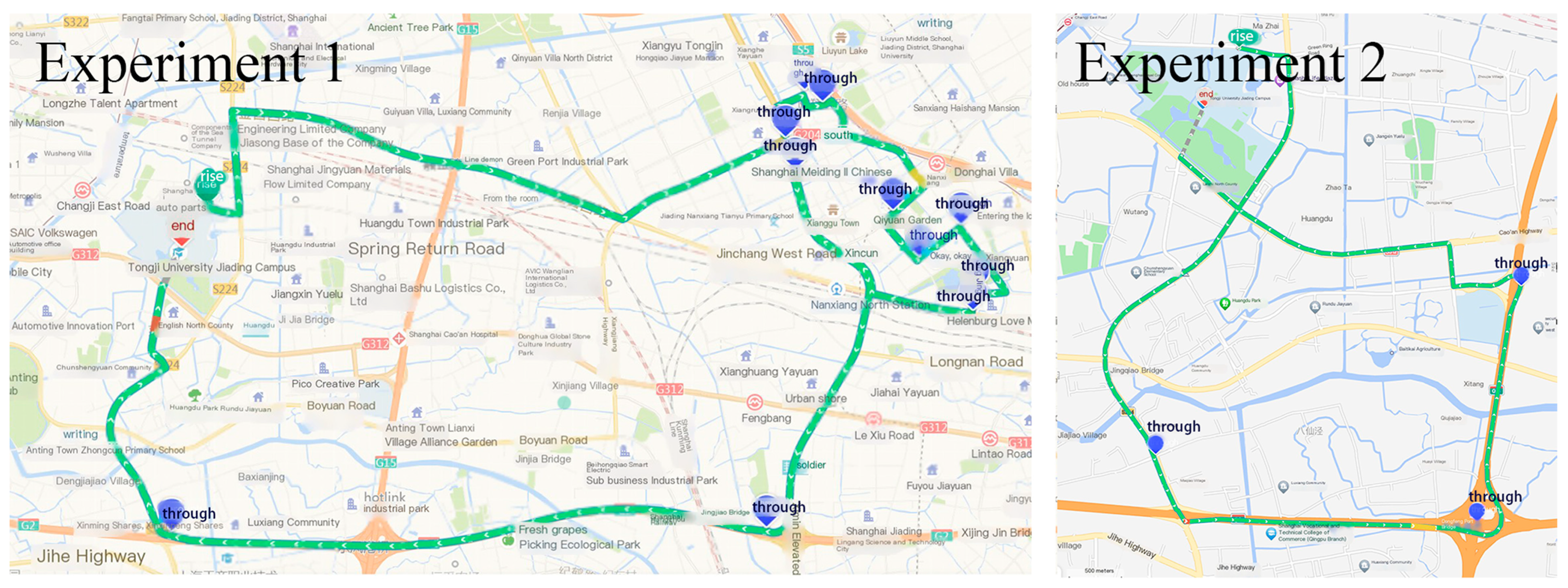
3.1. Overview of Experiments
3.2. Experimental Data
3.3. Data Preprocessing
4. Results and Discussions
4.1. Descriptive Statistical Analysis
4.1.1. Descriptive Statistical Analysis of Experiment 1
4.1.2. Descriptive Statistical Analysis of Experiment 2
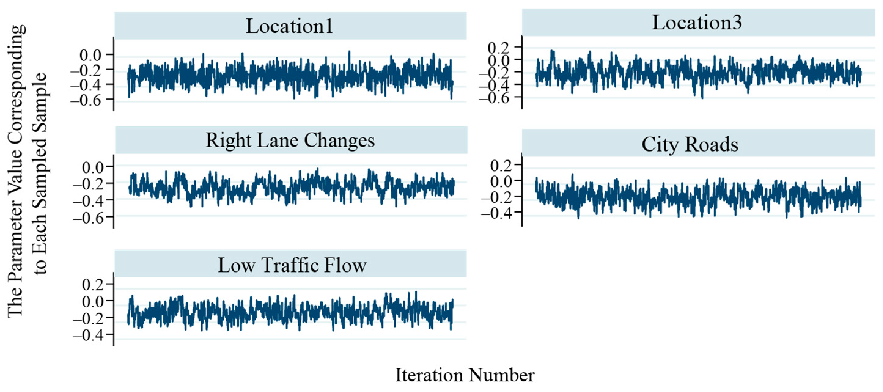
4.2. Bayesian Logistic Ordinal Regressions
4.2.1. Results and Analysis of Experiment 1
- 1.
- Driver Behavior:
- 2.
- Traffic Environment:
- 3.
- Blind Spot Imaging Design:
4.2.2. Results and Analysis of Experiment 2
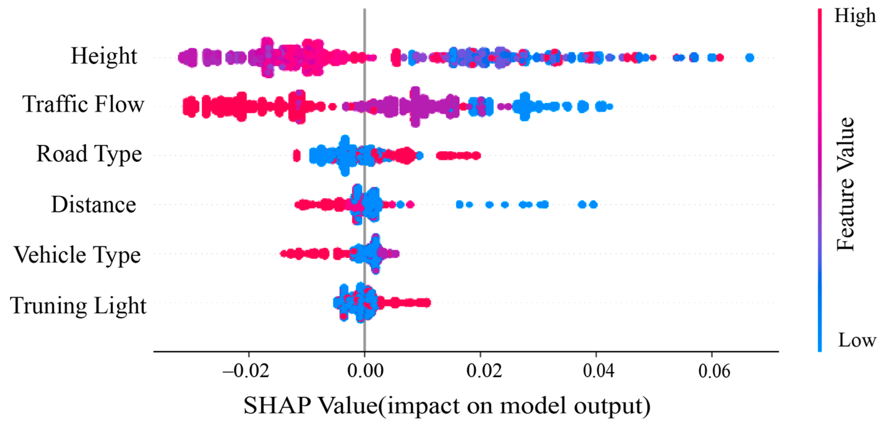
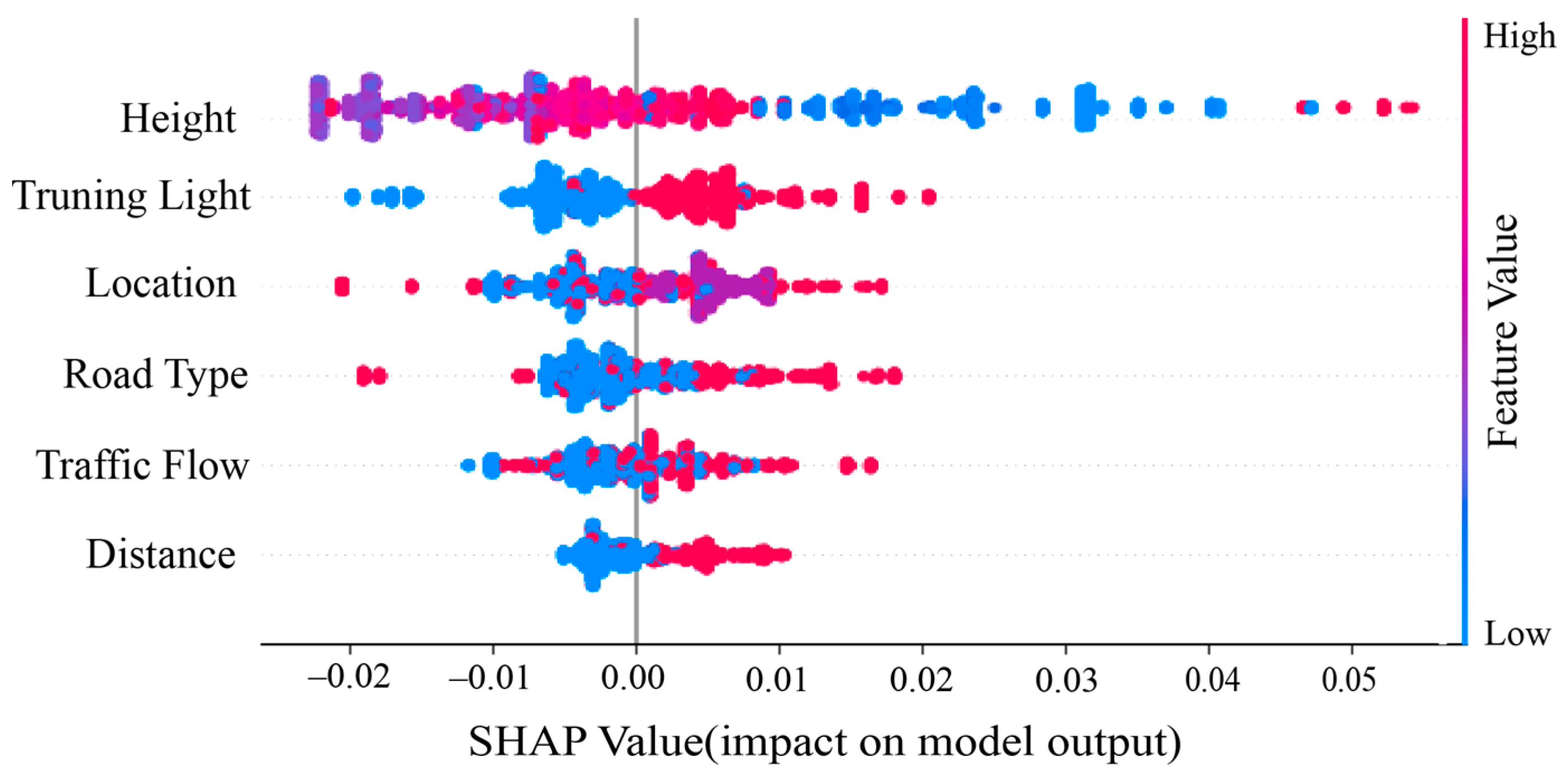
4.3. Impact Factor Analysiss
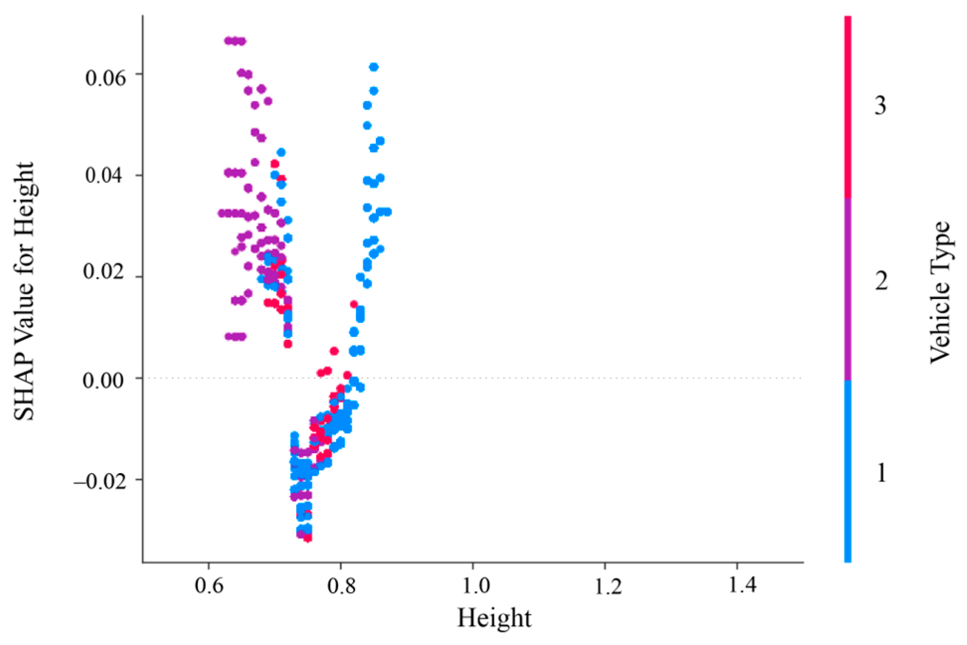
4.3.1. The Effect of Individual Characteristic Factors on Cognitive Load
- 1.
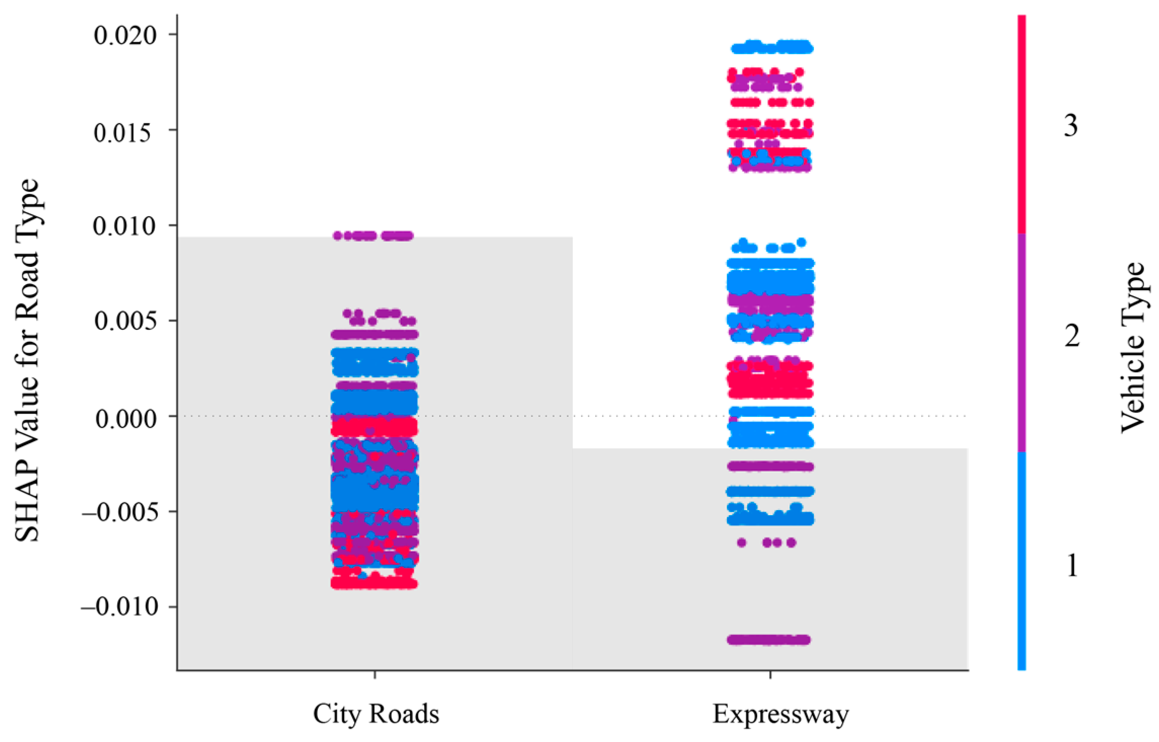
- Vehicle Type:
- 2.
- Blind Spot Design Features:
- 3.
- Environmental Factors:
- 4.
- Driver Characteristics:
4.3.2. Interaction Effects
5. Conclusions
Author Contributions
Funding
Institutional Review Board Statement
Informed Consent Statement
Data Availability Statement
Acknowledgments
Conflicts of Interest
References
- Václaviková, I.; Holienková, J.; Selecká, L. Global status report on road safety 2023. In Health and Safety; World Health Organization: Geneva, Switzerland, 2023; pp. 15–16. [Google Scholar]
- Zhang, T.; Chan, A.H.S. The association between driving anger and driving outcomes: A meta-analysis of evidence from the past twenty years. Accid. Anal. Prev. 2016, 90, 50–62. [Google Scholar] [CrossRef] [PubMed]
- Shawky, M. Factors affecting lane change crashes. IATSS Res. 2020, 44, 155–161. [Google Scholar] [CrossRef]
- Piccinini, G.; Simoes, A.; Rodrigues, C. Focusing on Drivers’ Opinions and Road Safety Impact of Blind Spot Information System (BLIS). In Advances in Human Aspects of Road and Rail Transportation; CRC Press: Boca Raton, FL, USA, 2013; pp. 57–66. [Google Scholar]
- Hargis, E. Blind Spot Accidents: Everything You Need to Know. Available online: https://www.lilawyer.com/blog/blind-spot-accidents/ (accessed on 10 April 2024).
- Hatamleh, H.; Sharadqeh, A.A.M.; Alnaser, A.a.M.; Alheyasat, O.; Abu-Ein, A.A.-K. Computer Simulation to Detect the Blind Spots in Automobiles. Int. J. Comput. Sci. Issues 2013, 10, 453–456. [Google Scholar]
- Chun, J.; Lee, I.; Park, G.; Seo, J.; Choi, S.; Han, S.H. Efficacy of haptic blind spot warnings applied through a steering wheel or a seatbelt. Transp. Res. Part F Psychol. Behav. 2013, 21, 231–241. [Google Scholar] [CrossRef]
- Fitch, G.M.; Lee, S.E.; Klauer, S.; Hankey, J.; Sudweeks, J.; Dingus, T. Analysis of Lane-Change Crashes and Near-Crashes; Report No. DOT HS 811 147; National Highway Traffic Safety Administration: Washington, DC, USA, 2009.
- Cicchino, J.B. Effects of blind spot monitoring systems on police-reported lane-change crashes. Traffic Inj. Prev. 2018, 19, 615–622. [Google Scholar] [CrossRef] [PubMed]
- Das Chakladar, D.; Roy, P.P. Cognitive Workload Estimation Using Physiological Measures: A Review; Indian Inst Technol Roorkee, Dept Comp Sci & Engn: Roorkee, India, 2023. [Google Scholar] [CrossRef]
- Hart, S.G.; Staveland, L.E. Development of NASA-TLX (Task Load Index): Results of Empirical and Theoretical Research. Adv. Psychol. 1988, 52, 139–183. [Google Scholar] [CrossRef]
- Reid, G.B.; Nygren, T.E. The Subjective Workload Assessment Technique: A scaling procedure for measuring mental workload. Hum. Ment. Workload 1988, 52, 185–218. [Google Scholar]
- Mariel, G.; Elke, V.; von Leupoldt, A.; Mittelstädt, J.M.; Van den Bergh, O. Respiratory Changes in Response to Cognitive Load: A Systematic Review. Neural Plast. 2016, 2016, 8146809. [Google Scholar]
- Veltman, J.A. A Comparative Study of Psychophysiological Reactions during Simulator and Real Flight. Int. J. Aviat. Psychol. 2002, 12, 33–48. [Google Scholar] [CrossRef]
- Palinko, O.; Kun, A.L.; Shyrokov, A.; Heeman, P. Estimating cognitive load using remote eye tracking in a driving simulator. In Proceedings of the Eye-Tracking Research & Applications, Austin, TX, USA, 22–24 March 2010. [Google Scholar]
- Prabhakar, G.; Mukhopadhyay, A.; Murthy, L.; Modiksha, M.; Sachin, D.; Biswas, P. Cognitive load estimation using ocular parameters in automotive. Transp. Eng. 2020, 2, 100008. [Google Scholar] [CrossRef]
- Desok, K.; Yunhwan, S.; Hyang-Sook, K.; Jung, S. Short term analysis of long term patterns of heart rate variability in subjects under mental stress. In Proceedings of the 2008 International Conference on BioMedical Engineering and Informatics, Sanya, China, 27–30 May 2008. [Google Scholar]
- Andreas, H.; Kati, H.; Anu, H.; Jussi, K.; Kiti, M. Mental workload classification using heart rate metrics. In Proceedings of the 2009 Annual International Conference of the IEEE Engineering in Medicine and Biology Society, Minneapolis, MN, USA, 3–6 September 2009; Annual Conference. IEEE Engineering in Medicine and Biology Society: New York, NY, USA, 2009; Volume 2009, pp. 1836–1839. [Google Scholar]
- Boring, M.J.; Ridgeway, K.; Shvartsman, M.; Jonker, T.R. Continuous decoding of cognitive load from electroencephalography reveals task-general and task-specific correlates. J. Neural Eng. 2020, 17, 056016. [Google Scholar] [CrossRef]
- Murtazina, M.; Avdeenko, T. Measuring cognitive load based on EEG data in the intelligent learning systems. In Proceedings of the SLET-2020: International Scientific Conference on Innovative Approaches to the Application of Digital Technologies in Education, Stavropol, Russia, 12–13 November 2020; CEUR Workshop Proceedings: Tenerife, Spain, 2020; Volume 2861, pp. 342–350. [Google Scholar]
- Gogna, Y.; Tiwari, S.; Singla, R. Mental Workload Assessment of Gamers’ Eeg with Multi-Domain Feature-Based Cognitive Model and Its Validation. Biomed. Eng. Appl. Basis Commun. 2024, 36, 2450022. [Google Scholar] [CrossRef]
- Luque, F.; Armada, V.; Piovano, L.; Barba, R.J.; Santamaría, A. Understanding Pedestrian Cognition Workload in Traffic Environments Using Virtual Reality and Electroencephalography. Electronics 2024, 13, 1453. [Google Scholar] [CrossRef]
- Bulumulle, G.; Boloni, L. A study of the automobile blind-spots’ spatial dimensions and angle of orientation on side-sweep accidents. In Proceedings of the 2016 Symposium on Theory of Modeling and Simulation (TMS-DEVS), Pasadena, CA, USA, 3–6 April 2016. [Google Scholar]
- Chong, I.; Mirchi, T.; Silva, H.I.; Strybel, T.Z. Auditory and Visual Peripheral Detection Tasks and the Lane Change Test with High and Low Cognitive Load. Proc. Hum. Factors Ergon. Soc. Annu. Meet. 2014, 58, 2180–2184. [Google Scholar] [CrossRef]
- Recarte, M.A.; Nunes, L.M. Mental workload while driving: Effects on visual search, discrimination, and decision making. J. Exp. Psychol. Appl. 2003, 9, 119–137. [Google Scholar] [CrossRef] [PubMed]
- Li, P.; Markkula, G.; Li, Y.; Merat, N. Is improved lane keeping during cognitive load caused by increased physical arousal or gaze concentration toward the road center? Accid. Anal. Prev. 2018, 117, 65–74. [Google Scholar] [CrossRef] [PubMed]
- Melnicuk, V.; Thompson, S.; Jennings, P.; Birrell, S. Effect of cognitive load on drivers’ State and task performance during automated driving: Introducing a novel method for determining stabilisation time following take-over of control. Accident Anal. Prev. 2021, 151, 105967. [Google Scholar] [CrossRef] [PubMed]
- Barkana, Y.; Zadok, D.; Morad, Y.; Avni, I. Visual field attention is reduced by concomitant hands-free conversation on a cellular telephone. Am. J. Ophthalmol. 2004, 138, 347–353. [Google Scholar] [CrossRef]
- Seppelt, B.; Seaman, S.; Angell, L.; Mehler, B.; Reimer, B. Differentiating Cognitive Load Using a Modified Version of AttenD. In Proceedings of the Automotive User Interfaces and Interactive Vehicular Applications, Oldenburg, Germany, 24–27 September 2017. [Google Scholar]
- Lechner, G.; Fellmann, M.; Festl, A.; Kaiser, C.; Kalayci, T.E.; Spitzer, M.; Stocker, A. A Lightweight Framework for Multi-device Integration and Multi-sensor Fusion to Explore Driver Distraction. In Proceedings of the Advanced Information Systems Engineering: 31st International Conference, CAiSE 2019, Rome, Italy, 3–7 June 2019; Springer International Publishing: Cham, Switzerland, 2019; Volume 11483, pp. 80–95. [Google Scholar] [CrossRef]
- Xu, J.; Qian, C.; Han, S.; Guo, F. Detecting Critical Mismatched Driver Visual Attention during Lane Change: An Embedding Kernel Algorithm. In IEEE Transactions on Intelligent Transportation Systems; IEEE: New York, NY, USA, 2024; pp. 1–11. [Google Scholar] [CrossRef]
- Yuki, M.; Tomonori, O.; Yoshiaki, M.; Daichi, S.; Meiko, M.; Miwa, N. Effects of Placing a CMS Monitor to Present Side and Rear View at the Driver-centered Position on Drivers’ Rearward Visual Behavior, Cognitive Load, and Mental Stress. Int. J. Automot. Eng. 2022, 13, 196–205. [Google Scholar]
- Regan, M.; Victor, T.; Lee, J. Chapter 19: The Driver Distraction Detection Algorithm AttenD. In Driver Distraction and Inattention; Advances in Research and Countermeasures; CRC Press: Boca Raton, FL, USA, 2013; Volume 1. [Google Scholar]
- Iddrisu, W.A.; Gyabaah, O. Identifying factors associated with child malnutrition in Ghana: A cross-sectional study using Bayesian multilevel ordinal logistic regression approach. BMJ Open 2023, 13, e075723. [Google Scholar] [CrossRef]
- Soda, M.A.; Hamuli, E.K.; Batina, S.A.; Kandala, N.-B. Determinants and spatial factors of anemia in women of reproductive age in Democratic Republic of Congo (drc): A Bayesian multilevel ordinal logistic regression model approach. BMC Public Health 2024, 24, 202. [Google Scholar] [CrossRef] [PubMed]
- Montesinos-López, O.A.; Montesinos-López, A.; Crossa, J.; Burgueño, J.; Eskridge, K. Genomic-Enabled Prediction of Ordinal Data with Bayesian Logistic Ordinal Regression. G3 Genes Genomes Genet. 2015, 5, 2113–2126. [Google Scholar] [CrossRef] [PubMed]
- Gianola, D.; Foulley, J. Sire evaluation for ordered categorical data with a threshold model. Genet. Sel. Evol. 1983, 15, 201–224. [Google Scholar] [CrossRef]
- Zhiwen, G.; Sheng, F.; Changchang, M.; Kai, W.; Kan, H.; Weijie, Z.; Xiaojun, D.; Lufang, F.; Jinghao, H. Quantifying and comparing the effects of key chemical descriptors on metal–organic frameworks water stability with CatBoost and SHAP. Microchem. J. 2024, 196, 109625. [Google Scholar]
- Zahid, M.; Habib, M.F.; Ijaz, M.; Ameer, I.; Ullah, I.; Ahmed, T.; He, Z. Factors affecting injury severity in motorcycle crashes: Different age groups analysis using Catboost and SHAP techniques. Traffic Inj. Prev. 2024, 25, 472–481. [Google Scholar] [CrossRef]
- Yao, Z.; Chen, M.; Zhan, J.; Zhuang, J.; Sun, Y.; Yu, Q.; Yu, Z. Refined Landslide Susceptibility Mapping by Integrating the SHAP-CatBoost Model and InSAR Observations: A Case Study of Lishui, Southern China. Appl. Sci. 2023, 13, 12817. [Google Scholar] [CrossRef]
- Prokhorenkova, L.; Gusev, G.; Vorobev, A.; Dorogush, A.V.; Gulin, A. CatBoost: Unbiased boosting with categorical features. Adv. Neural Inf. Process. Syst. 2019, 31. [Google Scholar] [CrossRef]
- Dureckova, H.; Krykunov, M.; Aghaji, M.Z.; Woo, T.K. Robust Machine Learning Models for Predicting High CO2 Working Capacity and CO2/H2 Selectivity of Gas Adsorption in Metal Organic Frameworks for Precombustion Carbon Capture. J. Phys. Chem. C 2019, 123, 4133–4139. [Google Scholar] [CrossRef]
- Lundberg, S.; Lee, S.-I. A unified approach to interpreting model predictions. In Proceedings of the 2017 Neural Information Processing Systems (NIPS) Conference, Long Beach, CA, USA, 4–9 December 2017. [Google Scholar]
- Szumska, E.M.; Grabski, P.T. An analysis of the impact of the driver’s height on their visual field range. In Proceedings of the 2018 XI International Science-Technical Conference Automotive Safety, Casta, Slovakia, 18–20 April 2018. [Google Scholar]


| Indicator | Explanations |
|---|---|
| Gaze Landing Point Coordinates | Taking the upper left corner of the HRT’s foreground video as the origin, the horizontal and vertical pixel distances corresponding to the driver’s gaze are output. These are used in the calculation of the time buffer value within the AttenD algorithm. |
| Head Rotation Angle | The left–right head rotation angles captured by the eye-tracker, which serve as auxiliary data for the calculation of the time buffer value. |
| Eye Height | The z-axis coordinate of the driver’s gaze origin position, as output by the eye-tracker in the world coordinate system. |
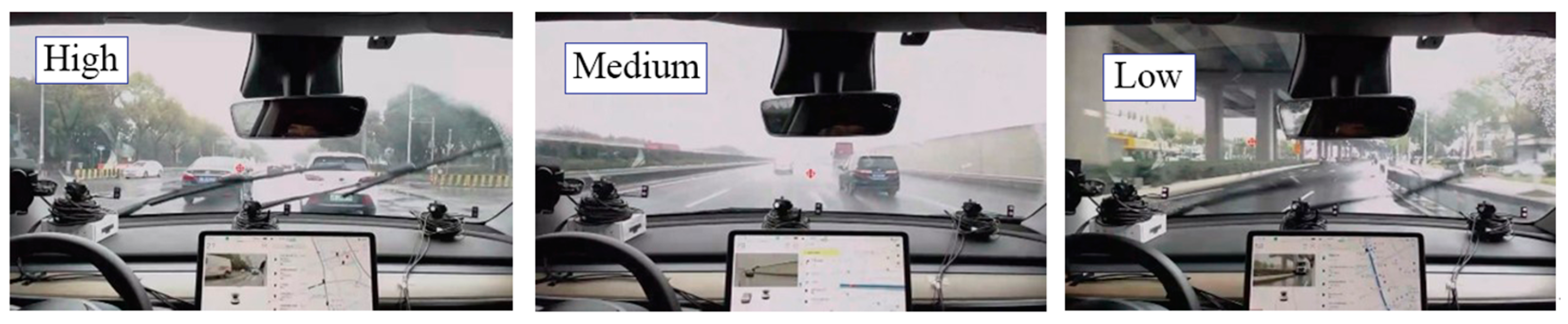
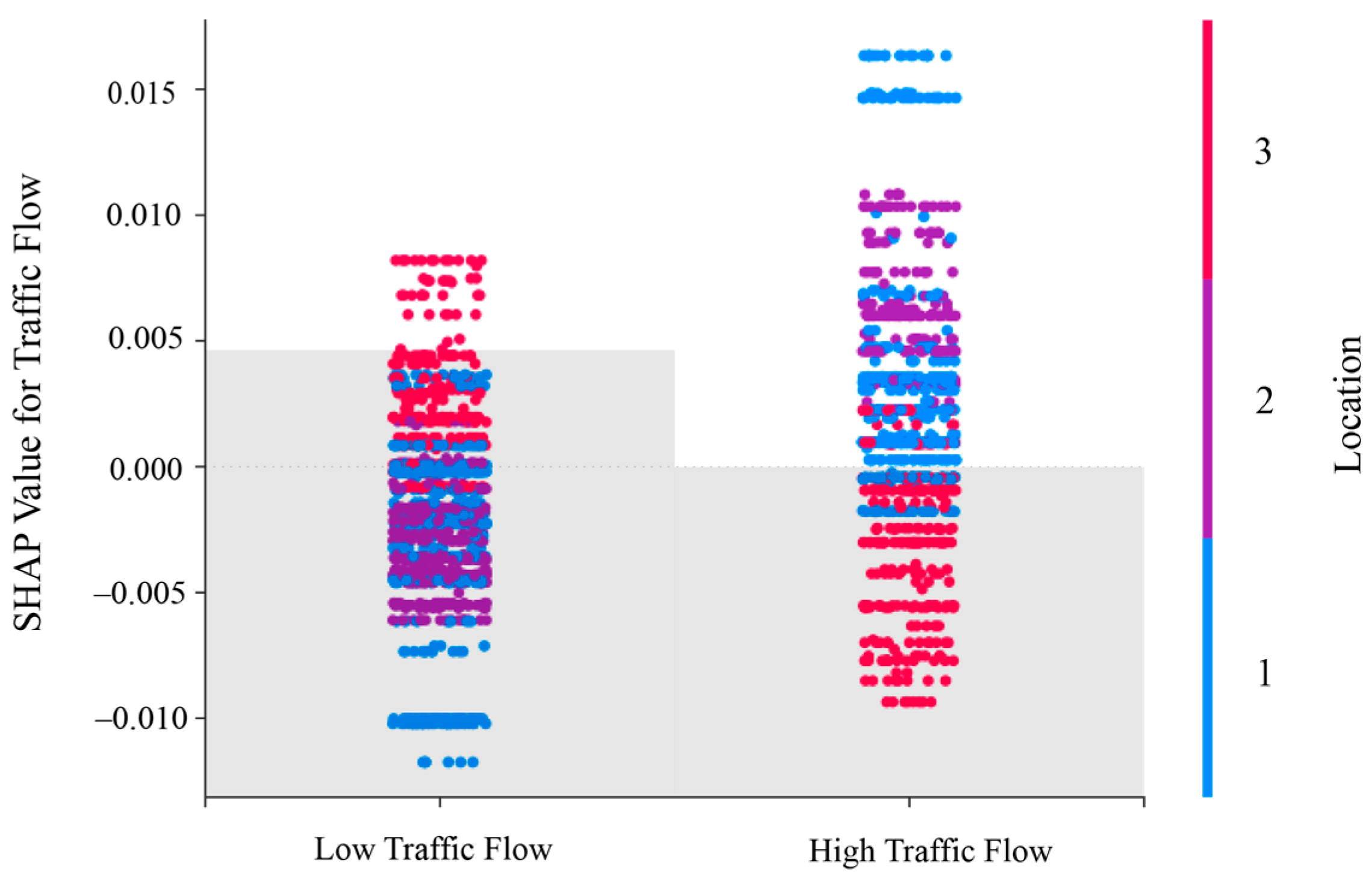
| Traffic Flow Level | Based on the volume of vehicles ahead on the road, traffic flow is classified into three levels: high, medium, and low. An example of traffic flow levels is illustrated in Figure 7. |
| Road Type | The type of road where the vehicle was located during data collection, categorized as city roads or expressways. |
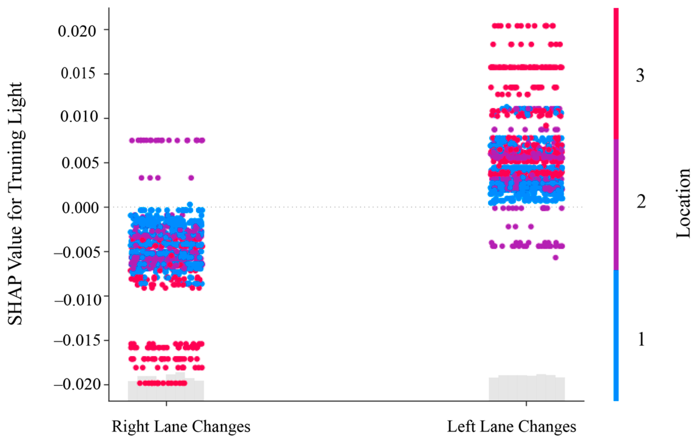
| Lane Change Direction | The direction of lane change (left or right) corresponding to each data entry. |
| Vehicle Type | As mentioned in Section 4.1, the vehicle type was analyzed as an overall variable to examine its impact on cognitive load in Experiment 1. Relevant parameters of the three vehicle types are presented in Table 2, where represents the ratio of the blind zone image to the center screen and D represents the horizontal distance from the left end of the blind zone image to the center of the steering wheel. |
| Blind Zone Image Position | As mentioned in Section 4.1, three positions of blind zone images of the first type of vehicles are selected for further experiments to analyze the influence of the blind zone image positions on the driver’s cognitive load. Relevant parameters of the three positions are presented in Table 3, where D represents the horizontal distance from the left end of the blind zone image to the center of the steering wheel, D1 represents the distance from the left end of the blind zone image to the left of the center screen, and D2 represents the distance from the top of the blind zone image to the top of the center screen. |
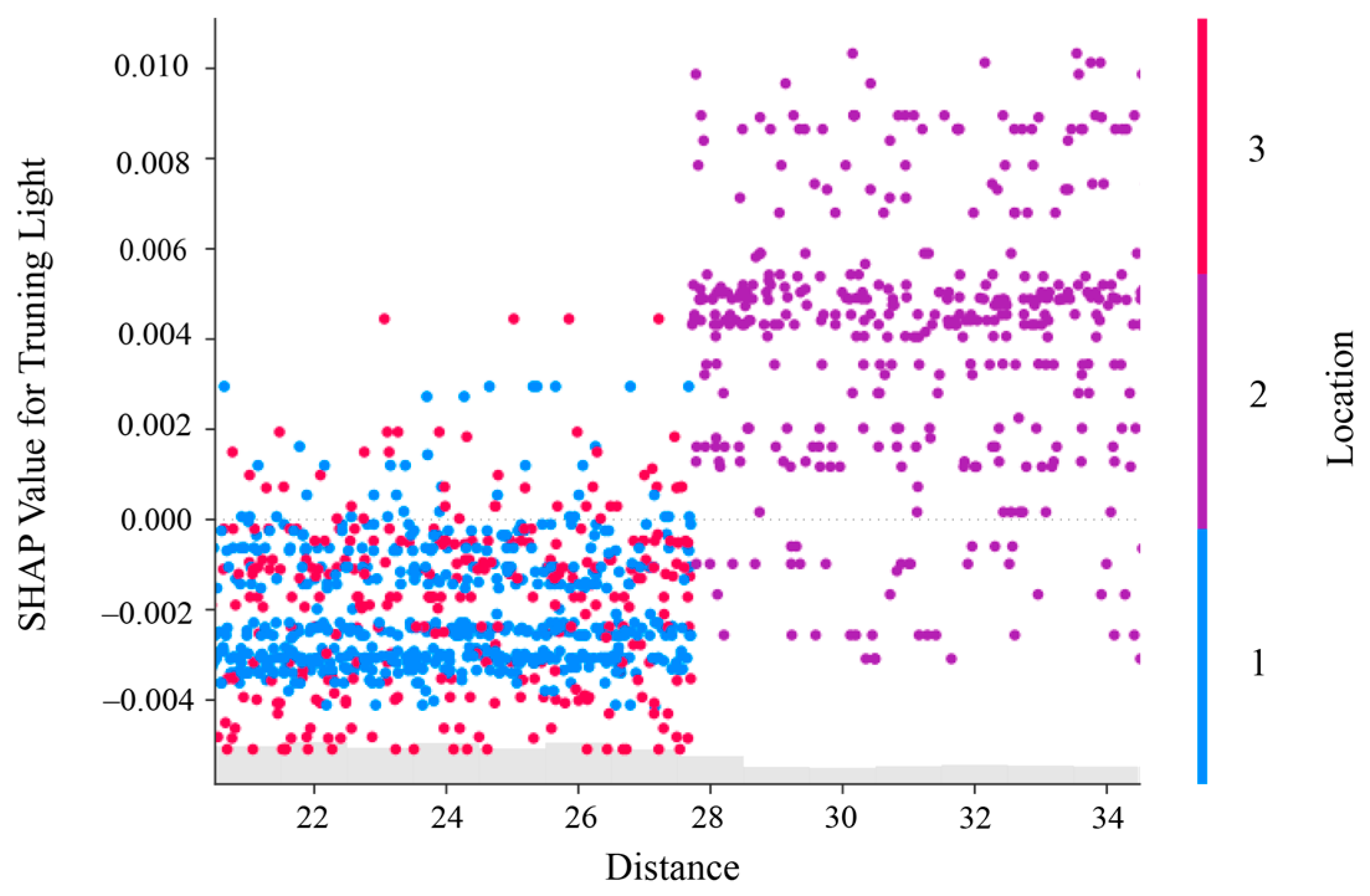
| Horizontal Distance of the Left End of the Blind Zone Image from the Center of the Steering Wheel | Since the distance of the blind spot from the driver’s eyes is positively correlated with its distance from the center of the steering wheel, and the driver’s head will rotate to a certain extent during the driving process, it is difficult to measure the distance from the eyes to the blind spot directly. Therefore, this study measured the distance from the left end of the blind spot to the center of the steering wheel, which was combined with the height of the driver’s line of sight to reflect the effect of the distance from the driver’s eyes to the blind spot on the driver’s cognitive load. Relevant parameters have been listed in Table 2 and Table 3. |
| Vehicle Type | Center Screen | Blind Zone Image | D/cm | |||||
|---|---|---|---|---|---|---|---|---|
| Length /cm | Width /cm | Area /cm2 | Length /cm | Width /cm | Area /cm2 | |||
| 1 | 33.1 | 20.7 | 685.2 | 12 | 6.1 | 73.2 | 0.11 | 21.2 |
| 2 | 65.8 | 10.9 | 717.2 | L: 10.9 | 9.0 | L: 98.1 | L: 0.14 | L: 14.5 |
| R: 16.0 | R: 144.0 | R: 0.20 | R: 34.2 | |||||
| 3 | 21.8 | 23.9 | 521 | 12.2 | 7.2 | 87.8 | 0.17 | 38.0 |
| Vehicle Type | Position | D/cm | D1/cm | D2/cm |
|---|---|---|---|---|
| 1 | 1 | 21.2 | 0.3 | 3.5 |
| 2 | 34.2 | 13.3 | 1.0 | |
| 3 | 21.2 | 0.3 | 12.7 |
| p-Value of Veh-Mean | p-Value of Veh-Std. | Vehicle Type | Veh-Mean | Veh-Std. | Mean | Std. | |
|---|---|---|---|---|---|---|---|
| City Roads | 0.471 | 0.501 | 1 | 1.363 | 0.556 | 1.379 | 0.577 |
| 2 | 1.368 | 0.665 | |||||
| 3 | 1.406 | 0.511 | |||||
| Expressway | 0.026 | 0.041 | 1 | 1.522 | 0.438 | 1.685 | 0.326 |
| 2 | 1.828 | 0.214 | |||||
| 3 | 1.705 | 0.326 | |||||
| Right Lane Changes | 0.282 | 0.366 | 1 | 1.343 | 0.561 | 1.410 | 0.557 |
| 2 | 1.389 | 0.634 | |||||
| 3 | 1.497 | 0.476 | |||||
| Left Lane Changes | 0.309 | 0.506 | 1 | 1.508 | 0.459 | 1.594 | 0.383 |
| 2 | 1.798 | 0.26 | |||||
| 3 | 1.477 | 0.43 | |||||
| Medium Traffic Flow | 0.014 | 0.02 | 1 | 1.538 | 0.421 | 1.500 | 0.465 |
| 2 | 1.77 | 0.278 | |||||
| 3 | 1.191 | 0.697 | |||||
| High Traffic Flow | 0.096 | 0.226 | 1 | 1.156 | 0.699 | 1.347 | 0.602 |
| 2 | 1.278 | 0.739 | |||||
| 3 | 1.606 | 0.367 |
| p-Value of Veh-Mean | p-Value of Veh-Std. | Position | Veh-Mean | Veh-Std. | |
|---|---|---|---|---|---|
| City Roads | 0.197 | 0.294 | 1 | 1.391 | 0.548 |
| 2 | 1.534 | 0.424 | |||
| 3 | 1.344 | 0.563 | |||
| Expressway | 0.014 | 0.02 | 1 | 1.601 | 0.395 |
| 2 | 1.684 | 0.355 | |||
| 3 | 1.317 | 0.597 | |||
| Right Lane Changes | 0.208 | 0.165 | 1 | 1.418 | 0.533 |
| 2 | 1.443 | 0.464 | |||
| 3 | 1.191 | 0.661 | |||
| Left Lane Changes | 0.012 | 0.082 | 1 | 1.483 | 0.478 |
| 2 | 1.725 | 0.338 | |||
| 3 | 1.472 | 0.494 | |||
| Low Traffic Flow | 0.477 | 0.473 | 1 | 1.37 | 0.547 |
| 2 | 1.543 | 0.401 | |||
| 3 | 1.081 | 0.738 | |||
| Medium Traffic Flow | 0.918 | 0.95 | 1 | 1.587 | 0.404 |
| 2 | 1.585 | 0.405 | |||
| 3 | 1.592 | 0.387 | |||
| High Traffic Flow | 0.003 | 0.009 | 1 | 1.35 | 0.583 |
| 2 | 1.618 | 0.388 | |||
| 3 | 1.357 | 0.574 |
| Mean | Std. Dev. | MCSE | Median | [95% Cred. Interval] | ||
|---|---|---|---|---|---|---|
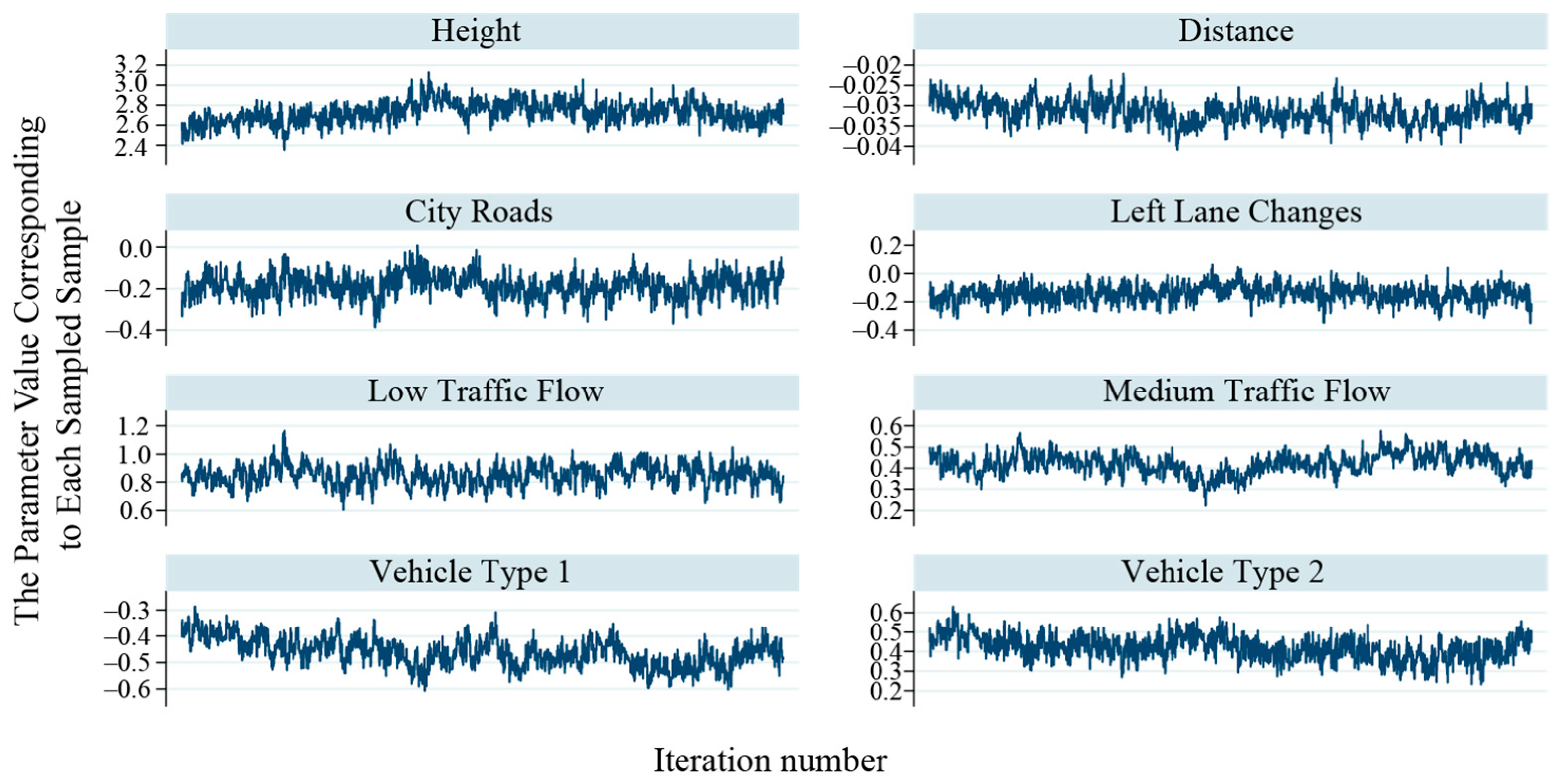
| Eye Height | 2.388 | 0.402 | 0.055 | 2.388 | 1.586 | 3.142 |
| Distance | −0.030 | 0.003 | 0.000 | −0.030 | −0.037 | −0.023 |
| City Roads | −0.203 | 0.051 | 0.004 | −0.203 | −0.302 | −0.104 |
| Left Lane Changes | 0.152 | 0.056 | 0.003 | 0.151 | 0.043 | 0.266 |
| Low Traffic Flow | 0.839 | 0.075 | 0.009 | 0.838 | 0.687 | 0.987 |
| Medium Traffic Flow | 0.419 | 0.054 | 0.006 | 0.420 | 0.302 | 0.520 |
| Vehicle Type 1 | −0.409 | 0.097 | 0.009 | -0.410 | −0.602 | −0.221 |
| Vehicle Type 2 | 0.429 | 0.087 | 0.006 | 0.431 | 0.259 | 0.595 |
| Mean | Std. Dev. | MCSE | Median | [95% Cred. Interval] | ||
|---|---|---|---|---|---|---|
| Location1 | −0.234 | 0.090 | 0.010 | −0.234 | −0.398 | −0.053 |
| Location3 | −0.188 | 0.095 | 0.006 | −0.189 | −0.373 | 0.007 |
| Right Lane Changes | −0.254 | 0.081 | 0.009 | −0.255 | −0.405 | −0.083 |
| City Roads | −0.150 | 0.091 | 0.008 | −0.149 | −0.330 | 0.033 |
| Low Traffic Flow | −0.082 | 0.078 | 0.004 | −0.084 | −0.230 | 0.081 |
Disclaimer/Publisher’s Note: The statements, opinions and data contained in all publications are solely those of the individual author(s) and contributor(s) and not of MDPI and/or the editor(s). MDPI and/or the editor(s) disclaim responsibility for any injury to people or property resulting from any ideas, methods, instructions or products referred to in the content. |
© 2024 by the authors. Licensee MDPI, Basel, Switzerland. This article is an open access article distributed under the terms and conditions of the Creative Commons Attribution (CC BY) license (https://creativecommons.org/licenses/by/4.0/).
Share and Cite
Cui, X.; Li, Y.; Yue, L.; Chen, H.; Zhou, Z. Investigating Blind Spot Design Effects on Drivers’ Cognitive Load with Lane Changing: A Comparative Experiment with Multiple Types of Intelligent Vehicles. Appl. Sci. 2024, 14, 7570. https://doi.org/10.3390/app14177570
Cui X, Li Y, Yue L, Chen H, Zhou Z. Investigating Blind Spot Design Effects on Drivers’ Cognitive Load with Lane Changing: A Comparative Experiment with Multiple Types of Intelligent Vehicles. Applied Sciences. 2024; 14(17):7570. https://doi.org/10.3390/app14177570
Chicago/Turabian StyleCui, Xiaoye, Yijie Li, Lishengsa Yue, Haoyu Chen, and Ziyou Zhou. 2024. "Investigating Blind Spot Design Effects on Drivers’ Cognitive Load with Lane Changing: A Comparative Experiment with Multiple Types of Intelligent Vehicles" Applied Sciences 14, no. 17: 7570. https://doi.org/10.3390/app14177570
APA StyleCui, X., Li, Y., Yue, L., Chen, H., & Zhou, Z. (2024). Investigating Blind Spot Design Effects on Drivers’ Cognitive Load with Lane Changing: A Comparative Experiment with Multiple Types of Intelligent Vehicles. Applied Sciences, 14(17), 7570. https://doi.org/10.3390/app14177570