Smart Internet of Things Power Meter for Industrial and Domestic Applications

Abstract

Considering the widespread presence of switching devices on the power grid (including renewable energy system inverters), network distortion is more prominent. To maximize network efficiency, our goal is to minimize these distortions. Measuring the voltage and current total harmonic distortion (THD) using power meters and other specific equipment, and assessing power factor and peak currents, represents a crucial step in creating an efficient and stable smart grid. In this paper, we propose a power meter capable for measuring both standard electrical parameters and power quality parameters such as the voltage and current total harmonic distortion factors. The resulting device is compact and DIN-rail-mountable, occupying only three modules in an electrical cabinet. It integrates both wired and wireless communication interfaces and multiple communication protocols, such as Modbus RTU/TCP and MQTT. A microSD card can be used to store the device configuration parameters and to record the measured values in case of network fault events, the device’s continuous operation being ensured by the integrated backup battery in this situations. The device was calibrated and tested against three industrial power meters: Siemens SENTRON PAC4200, Janitza UMG-96RM, and Phoenix Contact EEM-MA400, obtaining an overall average measurement error of only 1.22%.

1. Introduction

We are part of a rapidly developing society in which the pace of technological advancement is significant. New technologies such as Internet of Things (IoT), smart city solutions, self-driving vehicles, artificial intelligence (AI), blockchain, etc., enable the continual improvement of quality of life and the services we benefit from. The industrial environment is also developing at an accelerated pace, integrating new and smart technologies such as IoT, cyber–physical systems (CPS), cloud computing, machine learning (ML), and advanced simulation, all part of the Industry 4.0 revolution. Consequently, the energy sector is compelled to integrate new energy sources, particularly renewable ones, to meet growing consumption demands and reduce pollution. The power quality can be affected by network imbalances, the increasing number of new residential and industrial consumers, or the nonlinear loads [1].

1.1. General Concepts

At the moment, there is a high level of interest in measuring power quality at numerous points across an electrical grid to implement corrective measures where necessary. This trend has led to the development of new methods for identifying and classifying disturbances, employing complex mathematical procedures and deep learning techniques [2,3,4]. S.A. Deokar et al. [5] proposed a novel disturbances identification method based on discrete wavelet transform (DWT) and fast Fourier transform (FFT). Other methods involve the utilization of S-transforms or Hilbert–Huang transforms [6]. In the context where multiple disturbances can occur simultaneously in a network, after the identification stage, methods for classifying them are necessary. Shouxiang Wang et al. presented a solution to increase the accuracy of disturbance classification using deep convolutional neural networks [7].

Energy quality analysis is an important topic even for renewable energy producers, as they can face penalties from grid operators if they introduce imbalances into the system or even have their plants disconnected from the grid for a certain period [8]. A. Elkholy [9] measured the power quality parameters in 8 kWp photovoltaic plant connected to the low-voltage distribution network in Egypt and proposed mathematical models to characterize the current total harmonic distortion and the power factor. Several models of commercial solar inverters from multiple manufacturers were tested by Giuliano A. Rampinelli et al. [10] to model current distortions and power factor as a function of relative power. This model can be used in the sizing of inverters during the design stage and computerized simulation of photovoltaic plants.

Grid operators often face challenges in controlling various renewable energy sources due to their variable nature depending on environmental parameters such as sunlight, wind, and water. Forecasting models are used to estimate the power production and demand in the network [11]. Often, meteorological data are used to estimate the power quality parameters, as they play a key role in the forecasting process [12].

1.2. Research Perspective

From the research perspective, we tackle the following objectives and research questions:

• Discussing the importance of smart power meters capable of measuring higher-order harmonics, both on voltage and current;
• How would a flexible modular IoT-integrated smart meter architecture look like?
• Due to the high price and unavailability of calibration equipment, how can we empirically calibrate and compare a hardware device using other certified industrial equipment?

It is important to mention that the current paper offers the perspective of a proposed IoT-enabled smart meter architecture in the context of the continuously evolving smart grid domain. Our focus is oriented toward developing and building a cost-effective, small-size, flexible, and IoT-enabled smart meter. The focus of this paper is less oriented towards complex mathematical modeling, advanced algorithms, and compliance with various IEC industrial standards (that actually need specialized equipment).

The integration of power quality measurement solutions (industrial devices that measure not only active, reactive, and apparent power but also harmonic distortions in the grid) often requires the use of industrial protocols that predate the Industrial IoT era. These protocols, in addition to necessitating protocol adaptations (specialized gateways), introduce security vulnerabilities due to the unencrypted (clear text) transmission of data.

Moreover, although intelligent solutions for reporting consumed electrical energy (smart meters) exist and are compatible with IoT environments (e.g., capable of using MQTT for data transmission), they do not provide information regarding power quality (such as distortions, sudden voltage variations, and other parameters). Even when combining the two solutions—a power quality meter and a smart power consumption meter—space inefficiencies and, especially, cost considerations arise, and this combination still does not allow for a more complex analysis of current and voltage waveforms (e.g., for recognizing consumer patterns based on consumption signatures [13,14,15]).

In this paper, we propose, analyze, implement, and test an architecture for a smart power quality meter integrated into the IoT domain that has multiple advantages over existing commercial devices. Or solution is characterized by the following features:

• It is based on an open and well-known platform that can be programmed in C using freely available libraries and development environments (e.g., ESP32);
• It allows for both wireless and Bluetooth (integrated in the ESP32 MCU) connectivity;
• It supports local storage of measured data, including raw samples, on a microSD card in a text file;
• It enables connection via the RS485 interface within an industrial network;
• It supports the implementation of various communication protocols such as Modbus TCP/RTU and MQTT without being limited to these;
• It allows for local data processing and result aggregation;
• It supports varying the signal sampling rates;
• It enables continuous monitoring of the network, even in the absence of a grid voltage, by being powered by the integrated rechargeable backup battery;
• It supports the implementation of various encryption algorithms, with the microcontroller featuring a dedicated module for AES.

1.3. Research Methodology

The research methodology employed in our work is as follows:

• We reviewed the national legislation regarding power quality parameters (voltage, uptime, harmonics, etc.) that the grid operator needs to deliver to the clients;
• Conducting a thorough review and identifying the current interest in both the commercial and in the research field regarding smart power meters, integrating them in the Industrial IoT world and the importance of smart meters to domestic application;
• Identifying the technical characteristics that are scattered on various versions/products that would be a good solution to be merged together (e.g.,industrial protocols, wireless transmission, small-factor, battery-backed up, simple installation, flexible architecture);
• Reviewing various development platforms, demonstration boards, and test boards for the main components that can be used in the construction of the device to obtain the characteristics that we need;
• Proposing a flexible modular architecture that allows for using the best components while maintaining simplicity, cost-effectiveness, and small dimensions;
• Implementing at a test board level using development boards, breadboards, du-Pont wires, and other standard components typically used in prototyping;
• Designing and implementing the components on the PCB to achieve the previously mentioned characteristics;
• Programming and implementing a simple FFT-based solution for THD computation;
• Running a linear calibration procedure using an industrial calibrated commercial device;
• Testing various scenarios and compiling the results by using multiple calibrated power quality meters;
• Comparing the results and issuing opinions and conclusions based on the results obtained;
• Identifying improvement solutions to ensure compliance with specific international technical standards.

2. Related Work

Identifying disturbances is generally achieved using dedicated industrial equipment called power quality analyzers. Typically, these are installed at the grid connection points of energy producers, whether they are fossil fuel-based, nuclear or renewable energy power plants, as well as large industrial consumer locations. Given their specialized nature and complexity, the cost of acquisition for these devices is significant, which has prevented their widespread installation among small consumers. Recently, there has been a growing interest in developing small and inexpensive devices capable of measuring both standard electrical parameters and power quality parameters, which can be installed in the locations of ordinary consumers. L Ashok Kumar et al. [16] proposed a smart energy meter capable of measuring the electrical network parameters and calculating the energy consumption and total harmonic distortion using Fast Fourier Transforms (FFTs). The current and voltage values are measured using dedicated sensors, processed using an Microchip ATmega328P microcontroller, and then transmitted to the ThingSpeak cloud platform. The resulting values are compared to a set of commercial meters, such as Fluke 317, Fluke 434, and Mecho 5760.

Md. Tanvir Ahammed et al. [17] proposed an IoT-based smart meter designed for households, which enables local and online monitoring of the electrical parameters. An Esspressif Systems ESP32 microcontroller was used for processing the data supplied by the Peacefair PZEM-004T energy monitor module and then to transmit the information to a database using the Wi-Fi interface. The device includes a load-clipping algorithm. A set of relays were used to cut off the power line and alarm the user if the peak-hour maximum power limit (remotely imposed by the grid operator) is exceeded.

To enhance the efficiency of energy consumption analysis in buildings, it is necessary to monitor the individual consumption of various consumers rather than solely monitoring the consumption of the entire network. M. Alonso-Rosa et al. [18] proposed a low-cost IoT sensor designed to measure the power quality at the input of electrical appliances. This device is based on an Analog Devices ADE7758 energy metering module connected to an Microchip ATmega328 microcontroller used for signal processing. The measurement data are sent to a cloud IoT platform (ThingSpeak) using an Espressif Systems ESP8266 microcontroller. The device was tested using specialized laboratory equipment, such as a programmable AC source and a programmable electronic load.

Industrial smart meters often prove to be too expensive for residential users, and for this reason, their installation is often overlooked during the design of a home’s electrical system. E. Viciana et al. [19] developed an inexpensive, open-source power meter, the openZmeter, capable of power quality and energy measurement. This device uses a precision voltage divider and Hall effect sensors to measure the grid voltage and current. The signals are sampled using an STMicroelectronics STM32 microcontroller and then sent to be processed to an ARM Linux board controller. A backup battery is included to power the device in under-voltage conditions. The Wi-Fi interface of the ARM controller allows a client to retrieve the measured data from the device’s web server. Several tests were conducted, including comparative measurements with an existing commercial solution (Circutor MYeBOX-1500) to demonstrate the accuracy of the proposed smart meter.

Smart power meters have also proven useful in microgrid systems, enabling efficient network management by monitoring production capacity and consumption requirements. V. Isanbaev et al. [20] conducted a study on monitoring various electrical parameters such as voltage, current, frequency, power, and total harmonic distortions in microgrid networks. The authors integrated an openZmeter device in a microgrid network composed of a hybrid solar–wind system and a set of typical household appliances. Finally, they analyzed the measured data and compared the profiles of each load consumer, highlighting the usefulness of smart meters in this type of network.

M. Carratù et al. state in [21] that smart meters play a crucial role in the implementation of a smart city. The authors also proposed an Advanced Metering Infrastructure (AMI) based on a smart electrical power meter. The prototype used the Analog Devices ADE7913 ADC, and the sample processing was carried out by an STMicroelectronics STM32 microcontroller. For data transmission, a 169 MHz wM-Bus radio module was used. The device was calibrated and tested using a Fluke 6105A Power Quality Calibrator to reduce the measurements error.

3. Proposed Solution

In this section, we propose a solution for a small and smart power meter capable of measuring power quality parameters, such as the voltage and current total harmonic distortion. We aimed to design a user friendly device that can be easily installed in existing domestic or industrial power cabinets. In the following sections, we elaborate on both the hardware and software architectures, as well as the solutions adopted for various encountered technical challenges.

3.1. Hardware Architecture

Examining Figure 1, presenting the hardware architecture of the device, we can consider it to be composed of three main sections: the power supply, the data conditioning and acquisition, and the data processing and user interaction circuits.

The first section ensures the device’s power supply from both the electricity grid network and a backup battery in case of power outages or grid faults. The switching between the two power sources, the AC/DC Power Supply (5V) and the Backup Battery, is performed automatically by a specialized circuit without interrupting the device’s functionality. Regardless of the primary voltage source used, its output voltage must be adapted to the acceptable range for the rest of the circuit components. Responsible for this task is a buck-boost converter, the Main Power Supply (3.5V) block.

The second section of the architecture contains the Voltage sensing circuit and Current sensing circuit, circuits responsible for transforming the two physical quantities of interest into a voltage signal that can be interpreted by the next. The Signal conditioning circuit blocks adapt the output of the sensing circuits using a set of operational amplifiers (Op-Amp) and then feed their output signal to the data acquisition block, the ADC block, which was implemented using an analogue-to-digital converter, as the name states. Both ADC and Op-Amps require specific operating voltages generated by the Positive Voltage Supply (3 V) and the Negative Voltage Supply (−1.2 V) blocks, powered from the buck-boost converter presented in the previous section.

The digital information generated by the ADC is transmitted to the microcontroller through the SPI interface. Then, it makes them available to the user using multiple communication protocols: over the included Wi-Fi interface or the RS485 interface. The User interface elements block acts as a minimal Human-to-Machine (HMI) interface, including a set of LEDs and buttons physically accessible to the user who can use them to interact with the logic of the device. An SD card slot was added to allow for the logging of the acquired signal samples for an external, device-independent analysis.

3.1.1. Microcontroller

Given the technical requirements of the power meter, it was necessary to select a microcontroller equipped with at least the following components:

• Two SPI interfaces: one for the microSD card and one for the ADC communication (for parallelizing the communication tasks);
• One UART interface for the debug/programming port or the RS485 transceiver;
• Wi-Fi interface;
• Ten GPIOs for buttons, LEDs, battery charger, and other modules’ status or control signals;
• A 3.3 to 5 V supply voltage.

From the software point of view, a microcontroller with a high-frequency processor and a large amount of memory is needed. For accurate voltage and current measurements, a large number of signal samples are acquired using the ADC and stored in the microcontroller’s memory. Our goal is to analyze up to the 40th harmonic of the signal and calculate the total harmonic distortion (THD), which implies using a Fast Fourier Transformation (FFT) algorithm. Typically, these algorithms use large arrays of data and require significant computational power. The microcontroller needs to handle the data acquisition process, analyze the signal, calculate the required signal parameters, and serve the relevant values to one or multiple clients through the Wi-Fi and RS485 interfaces.

To select the appropriate microcontroller according to our requirements, we tested several current and largely available models from Espressif Systems and Raspberry Pi, such as ESP32 and Raspberry Pi Pico. On each model, we conducted several tests with different FFT algorithm libraries on the same input data set and measured the time required to complete the signal analysis. Then, we selected the model that executed the algorithm in the shortest time possible while also adhering to the hardware and software criteria imposed by us, as mentioned earlier. The detailed process and results of the benchmark are the subject of a scientific paper that is currently under development.

The selected microcontroller model was the Espressif Systems ESP32-WROVER-E-N16R8. It complies with the specifications imposed during the device design stage and is officially supported by PlatformIO, integrated in Visual Studio, Arduino IDE, and ESP IDF.

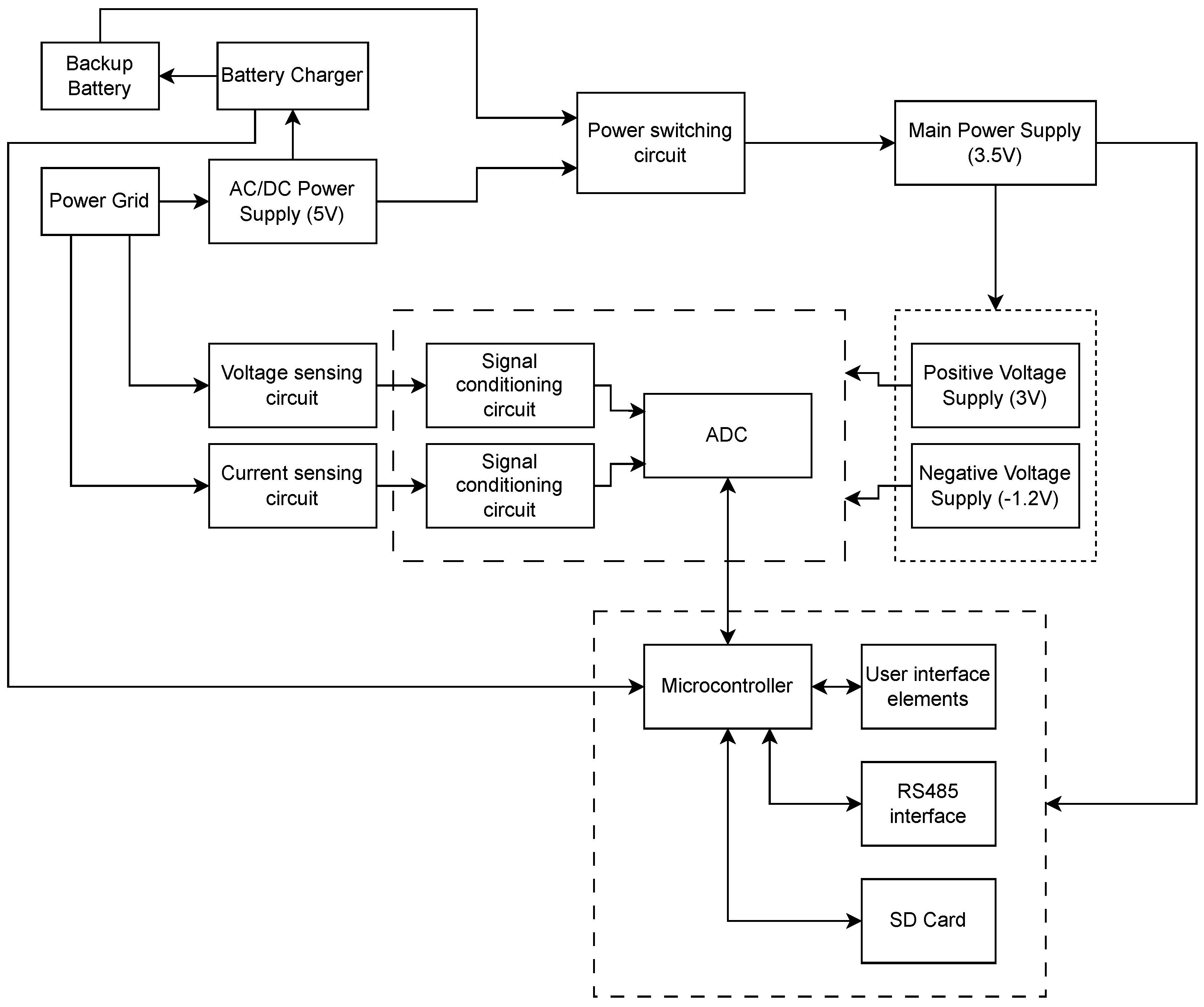
3.1.2. Power Supply: Main Power Supply, Battery Backup, and Overvoltage Protection

The power meter was designed to offer maximum functional availability. From the power supply perspective, this was achieved using a primary power source connected to the grid and a backup power supply represented by a rechargeable battery. The main power supply provides power to the device during normal operational conditions (grid voltage is present in the nominal range), and the battery is used only in emergency conditions (grid voltage absence, under or overvoltage).

To withstand the voltage variation of the grid, a wide input voltage range AC/DC converter was chosen: Multicomp MP-LD05-23B05R2. It accepts an input voltage range between 85 and 305 V AC, allowing the device to operate even in grid undervoltage and overvoltage scenarios. The 1 A output current (at 5 V) is sufficient for powering the internal circuits. A slow-acting, 2 A fuse and a varistor were added to protect the input side of the circuit, and an AC line filter reduces the unwanted grid noise. The power backup circuit was based on a 3.7 V, 620 mAh Li-Po battery connected to a specialized battery charging IC: Analog Devices MAX8903AETI+T. This circuit is connected to the 5 V output of the main power supply and charges the battery when the grid voltage is present.

A switching circuit based on PNP and P-MOS transistors was implemented to allow the device to be powered from the battery if the main supply becomes unavailable. The output generated by the energy source selecting circuit is then fed to the input of a buck-boost power supply, implemented with the ISL91127 from Renesas Electronics, that stabilizes the voltage at 3.5 V. To minimize the noise in the circuits, we used decoupling capacitors and ferrite beads.

The Op-Amps and ADC used in the signal conditioning and acquisition circuits require both a positive and a negative power supply. For the positive supply, a 3 V, 300 mA output current LDO voltage regulator was used: Texas Instruments TLV74330PDBVR.

The negative voltage was generated using a Texas Instruments LM2660 charge-pump voltage converter and then passed through a Microchip MIC5271 negative LDO regulator. The output voltage was set to −1.2 V and the maximum output current is 100 mA. Both circuits are powered from the main power supply.

3.1.3. Voltage and Current Conditioning Modules

To adapt the grid voltage and current values to the ADC maximum allowed input range of −1.3 V to 3.6 V, a specialized signal conditioning circuit was implemented. To reduce the voltage value, we used a voltage divider with a ratio of 301:1. The resulting voltage is passed through a buffer implemented using a Texas Instruments OPA388 operational amplifier. We selected this specific model for its characteristics: low noise, no crossover distortions, true rail-to-rail input and output, and 10 MHz gain bandwidth. Considering the ratio of the divider and the maximum range of the Op-Amp output (−1.2 V to 3 V), a maximum grid peak voltage of 361 V (approx. 256 V RMS) can be measured without saturating the amplifier.

To measure the current, we used a 500 $\mathsf{\mu }\mathsf{\Omega }$, 10 W shunt resistor. The resistor voltage drop is passed through a non-inverting amplifier, implemented with a Texas Instruments OPA388 Op-Amp. Considering the shunt resistor value and power rating, the amplifier gain (10), and the maximum range of the Op-Amp output, a maximum grid peak current of 141 A (approx. 100 A RMS) can be measured.

3.1.4. Signal Acquisition Module (ADC)

This application requires high-accuracy measurements of the grid voltage and current values. To achieve this, we used a Texas Instruments ADS131M04 analog-to-digital converter (ADC). It features 4 input differential channels, a 24 bit resolution, programmable data rate up to 64 kSPS, and a serial peripheral communication interface (SPI). We selected this 4-channel model due to the stock shortage of the 2-channel version (ADS131M02), while also considering potential future improvements of the device. Through the SPI interface, the microcontroller sends the ADC configuration commands and reads the values of the signal samples. To signal when new conversion data are ready in the internal registers, the ADC uses an active low digital output pin. We connected this pin to a hardware interrupt-capable input pin of the microcontroller so we could read the new ADC data as soon as they are available. The converter does not incorporate an internal clock generator; therefore, an external clock generator with a frequency of 8.192 MHz was added.

3.1.5. Data Logging and Transmission Interfaces

We considered that in case there is a grid overvoltage fault, it is useful to have the grid voltage and current waveforms recorded as proof. Using these data, one can demonstrate the fault to the grid operator and ask for material compensation if his appliances were damaged during the event. To provide an accessible way for the user to retrieve the data, we integrated a microSD memory card interface. It was connected to one of the microcontroller’s SPI interfaces to allow it to write the measured samples on the card and to read configuration parameters such as wireless network and remote data logging server connection settings. We also integrated an RS-485 interface using the MaxLinear SP3485CN RS-485 transceiver from MaxLinear. This interface is widely adopted in industrial environments due to its immunity to electromagnetic noise and allows for the connection of multiple devices on the same bus when a specialized communication protocol is used, such as Modbus RTU. To avoid transmission line impedance mismatch and to make sure that the line always remains in a well-defined state, we added termination and biasing resistors in the circuit that can be activated using dedicated dipswitches.

3.1.6. Device Assembly and PCBs

We need to mention that all of the electrical and electronic components, enclosures, and other parts used in building the presented device were supplied by Mouser Electronics, Inc., Mansfield, Texas, USA and Transfer Multisort Elektronik S.R.L., Timișoara, România and were shipped at our laboratory in Bucharest.

The device is designed for both industrial and home use to be easily installed into an existing electrical cabinet without requiring substantial changes to the electrical circuit. As we aimed for a compact device, we searched for a DIN rail-mountable enclosure that occupies a maximum of three slots.

A model that caught our attention was the Italtronix MODULBOX DIN 3M H53 (05.0302530), especially for its interior modularity. It has an exterior dimension of 90 mm × 53 mm × 58 mm (Lx × W × H) and can accommodate three stacked PCBs with the following sizes: 50.2 mm × 87 mm at the bottom, 49.7 mm × 58.7 mm in the middle, and 42 mm × 49.3 mm at the top of the case.

Considering this, the resulting physical circuit of the device was split into three boards, presented in Figure 2, one for each level of the case (from left to right):

• Bottom: contains the grid power supply, the voltage and current conditioning circuits, and the ADC module along with their positive and negative power supplies. On both short edges of this board, we placed a high-current screw terminal block, which allows for the connection of the grid or consumer conductors.
• Middle: includes the battery charger, power switching circuit, main power supply, the RS-485 transceiver, and the microcontroller.
• Top: contains the elements that need to be accessible to the user: the microSD card slot, the RS-485 wires connector and dipswitches for line termination and biasing, two push-buttons and two LEDs for user interaction, and a debug port for programming and testing purposes.

Figure 2. Device PCBs 3D view.

Figure 2. Device PCBs 3D view.

3.2. Software Architecture

Figure 3 illustrates the power meter’s software block diagram. As one can see, after each startup, the devices execute an initialization procedure, in which all the General-Purpose Input/Output (GPIO) pins are configured. Also, the Universal Asynchronous Receiver–Transmitter (UART) interface and Serial-Peripheral Interface (SPI) are configured and initialized to be used for the ADC, micro-SD card slot, debug/programming, and RS485 interfaces. After checking if a card is present, the device tries to read a standard configuration file from it, containing information about the Wi-Fi network (SSID and password) and other setting values such as time server information and communication protocol parameters. If the data are available and valid, they are further used by the algorithm; if not, a set of pre-programmed values are used instead.

If the Wi-Fi network connection is successful, the current timestamp is requested from a remote time server using the Network Time Protocol (NTP). If the response is valid, the current timestamp is used to name a new file that is created on the micro-SD card to store the signal samples for further analysis. If either the Wi-Fi or NTP fails, a generic name is used for the log file. After this step, a dedicated task running a Modbus protocol server is launched and used to serve information to the connected clients. The selection between the Modbus TCP and Modbus RTU protocols, used over the Wi-Fi or RS485 interface, is performed using a parameter stored in the configuration file read from the micro-SD card.

In the next steps, the ADC is initialized, and the acquisition completion (data ready) interrupt routine is activated, which is used by the microcontroller to read each data sample. After gathering the required number of data samples, the interrupt routine is deactivated temporarily until the values are processed. The algorithm computes the grid voltage and current RMS (root mean square) values and other grid parameters such as frequency and active and apparent power. A Fast Fourier Transform (FFT) algorithm is applied to the sampled data to extract the harmonics amplitude and calculate the total harmonic distortion (THD) values of the grid voltage and current. After this step, the Modbus protocol registers are updated with the new values, and if the configuration file dictates, the data are also transmitted via the Message Queuing Telemetry Transport (MQTT) protocol to a dedicated server for storage and further analysis. Before reactivating the ADC data ready interrupt routine, the data samples are written on the micro-SD card.

3.2.1. Sampled Data Storage and FFT Library Selection

The ADS131M04 ADC used in this device has a 24 bit resolution and a programmable sample rate between 250 SPS and 64 kSPS (kilo Samples Per Second). Given the 50 Hz frequency of the grid signal and the imposed requirement to analyze up the to 40th harmonic of the signal, for a correct FFT analysis, a minimum sample rate of 4 kSPS is necessary (40th harmonic frequency is 40 × 50 Hz = 2000 Hz but according to the Nyquist theorem, the sample rate should be at least twice this value, resulting in a minimum of 4000 Hz sampling frequency). In this case, the FFT produces 2000 frequency bins with a resolution of 1 Hz. According to the electrical standards [22], the grid frequency can vary between 49.8 and 50.2 Hz, and in this case, the sampled signal frequency components may not align perfectly with the FFT bins, causing a spectral leakage [23]. To overcome this issue, we can increase the sampling rate to 8 kSPS or 16 kSPS, achieving a resolution of 0.5 Hz or 0.25 Hz, respectively. Using this method, and applying a windowing function, helps in increasing the accuracy of harmonic amplitude estimation.

First, we need to store the voltage and current samples in the microcontroller’s memory before any computing occurs. For a given sampling period of 1 s, a sample rate of 8 kSPS, and the 24 bit resolution of the ADC, two arrays of 24,000 bytes are needed, one for each signal. According to the ESP32 documentation [24], “due to a technical limitation, the maximum statically allocated DRAM usage is 160 KB”. Moreover, the memory of the ESP32 is fragmented, making it impossible in some cases to allocate large-sized arrays. We came across this problem because the FFT libraries use large float buffers, usually with the dimension of the input data array. For example, in our case, for the same 1 s period and 8 kSPS sampling rate, at least two arrays of 8000 float variables would be needed for the FFT library input and output buffers. A float variable is represented using 32 bits (4 bytes), making it necessary to use 64,000 bytes only for the two arrays. To overcome this issue, we used PSRAM memory allocation for all the buffers, this feature being one of the main reasons why we selected the ESP32-Wrover model. We allocated memory for all the large buffers used in our algorithm and continued the initialization of the library used for the FFT analysis.

To select a suitable FFT library, we tested several commonly used libraries available in the Arduino Library Manager: ArduinoFFT, ESP32 FFT, Fast4ier, etc. Some of these were developed specifically for ESP32, while others were designed for different architectures (such as AVR) and were adapted by us to run on our microcontroller. The detailed testing procedure and the results obtained constitute the subject of another paper currently under development. We opted for the ESP32 FFT by Robin Scheibler library [25] because it produced the FFT analysis result in the shortest time compared to the other libraries tested. Additionally, it provides accurate estimations of harmonic amplitudes and fundamental frequency. Running this library on the ESP32-Wrover microcontroller, the average time required to finish the FFT analysis on a signal sampled at 8 kSPS for 1 s is 52.4 ms. The fundamental harmonic amplitude estimation error is 6.53%, and the frequency estimation error is 0.39%.

3.2.2. Calibration Procedure and Measured Value Calculation

To measure the power meter’s accuracy, we created a benchmarking setup using three industrial power meters: Siemens SENTRON PAC4200 (7KM4212-0BA00-3AA0, firmware v2.3.5) [26], Janitza UMG-96RM (52.22.001, firmware v3.13) [27], and Phoenix Contact EEM-MA400 (2901364, firmware U300-0002) [28]. These meters are capable of measuring the electrical properties of the network grid and to provide them to the user via the integrated display and communication interfaces. The Janitza and Phoenix Contact meters are equipped with RS485 serial interfaces and integrate the Modbus RTU protocol. Siemens SENTRON PAC4200 includes an Ethernet port and support the Modbus TCP protocol. For current measurements, we used the Lumel LCTR-5014500050A55 current transformer. According to the manufacturer [29], it features a primary current of 50 A and a secondary current of 5 A. It belongs to accuracy class 0.5 and operates at frequencies of 50/60 Hz. The transformer complies with the IEC 61869-1&2 standard [30,31] and provides a 14mm diameter hole to pass the conductor across, with which the current will be measured. The meter accuracy classes according to the IEC61557-12 standard [32] for various types of measurements are presented in

Table 1. Power meter accuracy classes comparison.

Measurement	Siemens PAC4200	Janitza UMG96-RM	Phoenix EEM-MA400
Phase Voltage	0.2	0.2	0.2
Phase Current	0.2	0.2	0.2
Frequency	0.1	0.05	0.1
Total Active Power	0.2	0.5	0.5
Total Reactive Power	1.0	1.0	0.5
Total Apparent Power	0.5	0.5	0.5
Voltage THD	2.0	1.0	Not specified
Current THD	2.0	1.0	Not specified

.

Both Siemens and Janitza power meters were updated to the last firmware version available at the time the tests were conducted, using their management software: SENTRON PowerConfig v3.27 and GridVis v9.1. For the Phoenix Contact meter, there was no update available. All the power meters were configured for single-phase measurements, and the without voltage transformer and current transformer ratio was set to 50 A/5 A. For the Siemens PAC4200 meter, we set a static IP address for the Ethernet interface and the 502 TCP port for the Modbus TCP protocol. For the Janitza UMG-96RM and Phoenix Contact meters, we set the RS485 interface parameters to 19,200 baud rate, 8 data bits, 1 stop bit, no parity. We assigned different Modbus addresses to allow for the unique identification of the devices on the bus.

For the calibration process, the three industrial power meters voltage input terminals were connected to our device’s load connector. Then, one of the load conductors was passed through the current transformers. This setup ensures that both voltage and current are measured at the same point in the circuit by all devices. The input voltage conductors, from the grid connector of the device, were connected to the output of an isolation transformer. The transformer has two outputs, each with different voltage levels (110 V and 230 V), which were sequentially used during the calibration process. At the load connector, a multi-socket extension cord was connected. This allows us to feed power to one or multiple loads and, as a result, to control the consumed and measured currents.

To achieve the best results, the grid voltage and the load current must be constant during the calibration process. For the voltage measurement calibration process, an APC SUA1500I Smart-UPS (Uninterruptible Power Supply) was interposed between the isolation transformer and the local grid connection (wall socket). This model generates a pure sine wave output, accepts an input voltage between 160 and 286 V, and has an output power of 980 W (1500 VA). During the tests, we discovered that the local grid voltage can fluctuate by up to 3 V within a 10-min interval, but using the UPS, we reduce the voltage variation to a maximum of 400 mV. To keep the load current stable during the calibration, we connected several incandescent light bulbs with different power ratings (40 W, 100 W, 200 W) and a 2500 W radiator, obtaining different load currents. The calibration setup is presented in Figure 4.

Using this setup, we applied a two-point calibration method for the voltage and current measurements. This method involves conducting two sets of measurements at different points using the device to be calibrated and another already calibrated device, serving as a reference [33,34,35,36,37]. We can establish a linear relationship between two known points, which can be correlated with (1).

$$y=m\times x+b$$

(1)

where

y represents the actual value (reference device),

m is the slope of the calibration curve (gain),

x represents the measured value (device to be calibrated), and

b is the curve y-intercept (offset).

The first measurement should be performed within the lower range of the device’s measurement domain, while the second measurement, if possible, should be executed within the upper range. For each measurement, the values indicated by both devices are recorded and then inserted into (2).

$$\begin{array}{c}\hfill Ou{t}_{val}=(Ra{w}_{val}-De{v}_L)\times {\displaystyle \frac{Re{f}_{range}}{De{v}_{range}}}+Re{f}_L\\ \hfill Re{f}_{range}=Re{f}_H-Re{f}_L\\ \hfill De{v}_{range}=De{v}_H-De{v}_L\end{array}$$

(2)

where

$Ra{w}_{val}$ is the value measured by the device at a given moment of time that needs to be corrected,

$De{v}_L$ represents the value measured in the lower end domain of the device that needs to be calibrated,

$De{v}_H$ is the value measured in the high-end domain of the device that needs to be calibrated,

$Re{f}_L$ represents the value measured in the lower-end domain of the calibrated (reference) device, and

$Re{f}_H$ is the value measured in the higher-end domain of the calibrated (reference) device.

We used as reference device the Siemens SENTRON PAC4200 power meter. For the voltage measurement calibration, we executed the first measurement connecting our measuring device to the 110 V output of the isolation transformer. We recorded the phase voltages indicated by the Siemens power meter and our device and then executed the second measurement using the 230 V output of the isolation transformer. We stored the parameters and then used them in the compensation equation to adjust each measured voltage sample. The same technique was used for the current measurement. Using the signal samples, we calculated the voltage and current RMS values using (3).

$$RM{S}_{value}[V/A]=\sqrt{{\displaystyle \frac{{\sum }_{i=1}^n{S}_i^2}{n}}}$$

(3)

where

$S_i$ represents the signal sample, and

n is the total number of samples.

The active power was calculated as the average value of the voltage and current samples product. The apparent power results as the product of the voltage and currentRMS values. Based on the active and apparent power, the reactive power and power factor was obtained using (4).

$$\begin{array}{c}\hfill P\left[W\right]={\displaystyle \frac{{\sum }_{j=1}^n{U}_j\times I_j}{n}}\\ \hfill S\left[VA\right]=U_{RMS}\times I_{RMS}\\ \hfill Q\left[VAr\right]=\sqrt{S^2-P^2}\\ \hfill PF={\displaystyle \frac{P}{S}}\end{array}$$

(4)

where:

$U_j$ represents a voltage sample value,

$I_j$ represents a current sample value,

n is the total number of samples,

$U_{RMS}$ is the voltage RMS value, and

$I_{RMS}$ is the current RMS value.

To analyze the power quality, we needed to compute the voltage and current total harmonic distortion values. This was achieved by determining the signal harmonic spectrum using a Fast Fourier Transform (FFT) and extracting the harmonics amplitude. The total harmonic distortion was calculated by introducing the harmonics amplitude in (5),

$$THD[\%]={\displaystyle \frac{\sqrt{{\sum }_{i=2}^n{H}_{iRMS}^2}}{H_{fRMS}}}\times 100\%$$

(5)

where:

n represents a maximum number of harmonics to be included in the analysis,

$H_{fRMS}$ represents the RMS amplitude of the fundamental harmonic, and

$H_{iRMS}$ represents the RMS amplitude of a harmonic component, other than the fundamental.

3.2.3. Measurement Data Acquisition Architecture

It was necessary to acquire and store the measured data from our device and the industrial power meters for the calibration process and for further analysis. To accomplish this task, we implemented a data aggregation system capable of converting the various communication protocols utilized by the measurement devices: the Siemens SENTRON PAC4200 power meter supports the Modbus TCP protocol, and the Janitza UMG-96RM and Phoenix Contact EEM-MA400 integrate the Modbus RTU protocol, and our device supports the Modbus TCP, RTU, and MQTT protocols. While for other devices, we utilized the Modbus protocol, and we opted to retrieve data from our device via the MQTT protocol. This choice was made due to MQTT’s widespread adoption in IoT applications and to test if it negatively affects the measurement process by introducing delays in data transmission.

To easily present, correlate, and analyze the measurement data gathered from all the devices, we decided to use Grafana, an open-source observability platform. A Raspberry Pi 5 single-board computer (8 GB RAM) was selected to serve as host for Grafana and for the InfluxDB database that will hold the measurement data gathered from the power meters. We installed the latest available 64-bit version of Raspberry Pi OS based on Debian 12 Linux, connected the system to the local Wi-Fi network, and then installed Grafana v10.4.0 and InfluxDB v1.8.10. Finally, we created a dashboard with trends for the measured values of interest (voltage, current, power, frequency, power factor, and THD).

To populate the database, we needed a method to convert the measured data acquired from the meters through the Modbus TCP/RTU and MQTT protocols. For this purpose, we used Node-RED, a flow-based programming tool. This programming environment was selected due to the availability of multiple libraries that offer support for InfluxDB database connectivity and various communication protocols, including Modbus and MQTT. We installed Node-RED v3.1.7 locally on a Raspberry Pi 3B+ single-board computer running the latest available 64-bit version of Raspberry Pi OS. This computer was also connected to the local Wi-Fi network using its Ethernet port to the Siemens PAC4200 power meter. The Janitza and Phoenix Contact power meters serial interfaces were connected to a two-port RS485-USB interface. Each serial port can be accessed independently by the operating system and the Node-RED program.

Each power meter, including our device, has a separate Node-RED flow responsible for periodically reading the measured data from the device using the Modbus RTU/TCP protocol (industrial meters) or MQTT (our device), converting the data and then inserting them into the database. For the MQTT protocol, a way to route the client’s messages was needed; therefore, we installed Mosquitto, an open-source MQTT message broker, on the Raspberry Pi 3B+ computer. Both our measuring device’s MQTT client and the client from the Node-RED data conversion flow connect to the broker and subscribe to the same topic. The communication between the single board computers and our meter is facilitated through the local network’s router, as it can be seen in Figure 4, and the diagram of the protocol conversion and message flow can be observed in Figure 5.

4. Results

To test the accuracy of out power meter and determine the measurement error, we implemented the setup described in Figure 4, removed the UPS and isolation transformer, and connected our device directly to the local grid. We installed the power meters and the auxiliary equipment inside a two-bay cabinet. A multiple socket outlet was mounted on the side of the cabinet to allow for the connection of different consumers. Figure 6 presents the layout of the cabinet:

• Industrial power meters,
• Our device,
• Current transformers,
• RS485-USB two-port serial interface,
• Raspberry Pi 3B+ computer.

Figure 6. Power meters cabinet.

Figure 6. Power meters cabinet.

We conducted multiple tests, over a period of several days, with the aim of creating different scenarios of electrical grid loading, connecting and disconnecting various loads:

• Incandescent bulbs (60 W, 100 W and 200 W),
• Oil radiator (heater) (2.5 kW),
• Bench grinder (250 W),
• Steam Iron (2 kW),
• Power resistor connected through a transformer,
• Faculty electronic lab workbench supply network (8 workbenches equipped with power supply, signal generator, oscilloscope, bench multimeter, desktop computer, and monitor).

During the tests, the power meters measurement data were logged in the database, plotted, and compared using Grafana. To determine the measurement error, we extracted the power meter data from the database as an average of the last 5 s values. For each data record and electrical property, we compared the value measured by our device with the values measured by each industrial meter and determined the measurement error using (6).

$$\begin{array}{c}\hfill Er{r}_{1M}[\%]={\displaystyle \frac{P{M}_{value}-I{M}_{value}}{I{M}_{value}}}\times 100\%\\ \hfill Er{r}_{3M}[\%]={\displaystyle \frac{P{M}_{value}-I{M}_{avg}}{I{M}_{avg}}}\times 100\%\\ \hfill I{M}_{avg}={\displaystyle \frac{JA{N}_{value}+PH{X}_{value}+SI{M}_{value}}{3}}\end{array}$$

(6)

where

$P{M}_{value}$ represents one measurement (value) from our meter,

$I{M}_{value}$ represents one measurement (value) from an industrial meter,

$JA{N}_{value}$ represents the Janitza UMG-96RM measured value,

$PH{X}_{value}$ represents the Phoenix Contact EEM-MA400 measured value,

$SI{M}_{value}$ represents the Siemens SENTRON PAC4200 measured value,

$Er{r}_{1M}$ is the measurement error between our meter and one industrial meter,

$Er{r}_{3M}$ is the measurement error between our meter and all other meters,

$I{M}_{avg}$ is the average value of the three industrial meters’ measurements.

4.1. Numerical Results

The measurement errors between the devices for each electrical property are displayed in

Table 2. Power meter (our solution) vs. industrial meter measurement errors.

Measurement	Measurement Error [%]
	Janitza UMG-96RM	Phoenix EEM-MA400	Siemens PAC4200	Average
Voltage	0.24	0.24	0.09	0.19
Current	0.14	0.59	0.44	0.30
Frequency	0.02	0.02	0.02	0.02
Power Factor	0.02	0.02	0.02	0.02
Active Power	0.37	0.74	0.36	0.24
Reactive Power	2.27	9.36	1.09	2.16
Apparent Power	0.38	0.73	0.36	0.27
Voltage THD	4.38	8.07	3.10	4.03
Current THD	5.08	7.75	2.85	3.79
Average	1.43	3.06	0.92	1.22

. Columns 2 to 4 presents the error between our meter and each industrial meter, and the average value of the three errors is calculated in the last column. The last line of the table presents the average of all electrical properties’ error values, which can be interpreted as general error values.

For a clearer analysis, we also compared the values measured by the industrial meters and determined the measurement errors between them using (7).

$$\begin{array}{c}\hfill Er{r}_{X-Y}[\%]={\displaystyle \frac{PM{X}_{value}-PM{Y}_{value}}{PM{Y}_{value}}}\times 100\%\\ \hfill AvgEr{r}_{XY}[\%]={\displaystyle \frac{Er{r}_{X-Y}+Er{r}_{Y-X}}{2}}\end{array}$$

(7)

where

$PM{X}_{value}$ and $PM{Y}_{value}$ are the values measured by different meters (X and Y),

$Er{r}_{X-Y}$ is the measurement error between meter X and meter Y (reference),

$AvgEr{r}_{XY}$ represents the average measurement error between two different meters.

Table 3. Industrial meters comparative measurement error.

Measurement	Measurement Error [%]
	JAN vs. PHX	PHX vs. JAN	JAN vs. SIM	SIM vs. JAN	PHX vs. SIM	SIM vs. PHX
Voltage	0.03	0.03	0.16	0.16	0.16	0.16
Current	0.73	0.72	0.57	0.57	0.15	0.15
Frequency	0.01	0.01	0.01	0.01	0.02	0.02
Power Factor	0.01	0.01	0.01	0.01	0.02	0.02
Reactive Power	11.89	10.57	3.06	2.98	8.50	9.36
Apparent Power	1.12	1.11	0.74	0.73	0.38	0.38
Voltage THD	7.74	7.78	1.59	1.62	7.45	7.62
Current THD	8.26	8.72	2.50	2.58	7.84	7.77
Average	3.43	3.34	1.04	1.04	2.77	2.87
	3.39		1.04		2.82
	JAN-PHX		JAN-SIM		PHX-SIM

JAN = Janitza UMG-96RM meter, PHX = Phoenix Contact EEM-MA400 meter, SIM = Siemens SENTRON PAC4200 meter.

presents the industrial meters’ comparative errors in columns 2 to 7. As can be seen, each device was taken sequentially as a reference for the other meters. Finally, the average error values between each pair of devices are calculated in the last row of the table.

From these results, we can observe that our device most closely aligns with the values measured by the Siemens SENTRON PAC4200 meter (0.92% error), which was expected given the fact that it was calibrated against it. We can also see that the Phoenix Contact meter presents the largest errors compared to the Siemens (2.82%) and Janitza (3.39%) meters, explaining why our power meter has the largest measurement error against this device (3.06%). The largest errors of our device can be observed in the case of THD measurements. They are a result of the FFT library harmonics amplitude estimation accuracy and can be improved by calibrating the voltage and current harmonic measurements with the reference meter’s values. Calibrating each measured electrical quantity would also reduce the overall error (1.22%), but this optimization was not applied as we aimed to determine the device’s real, unaltered performance.

Another important factor that negatively affects the measurement error is the inability to synchronize the sampling moment of the power meters. Each device has a different average interval for the measured values. Moreover, delays in updating the measured data in the database are introduced by the communication protocols and conversion steps described in Section 3.2.3.

Table 4. Reactive power samples comparison.

Sample	Phoenix EEM-MA400 [VAr]	Janitza UMG-96RM [VAr]	Siemens PAC4200 [VAr]	Power Meter [VAr]
1	30	33.308	32.236	32.480
2	30	33.433	32.338	32.526
3	30	33.900	32.680	32.932
4	30	33.950	32.792	33.113
5	87	88.890	91.590	88.740
6	78	87.702	90.455	86.994
7	76	88.294	91.017	87.719
8	82	88.643	91.314	87.692
9	82	89.831	92.350	88.681
10	80	90.879	93.385	89.763

presents a set of reactive power measurement samples gathered from the industrial meters and our device. As can be observed, the values measured by our device, Janitza, and Siemens meters are very similar, while the data collected from the Phoenix Contact power meter show a greater deviation. This behavior results from the way the devices scale and provide the measured values through the Modbus protocol. Our device and the Janitza and Siemens meters provide the reactive power value unscaled, as a float variable, stored in two Modbus Holding registers. The Phoenix Contact Meter offers the value scaled as kVAr/100, stored as an Int32 variable in two Modbus Holding registers. Since we aimed to store the data in the same format in the database, we converted the value received from the Phoenix Contact meter into VAr. As can be observed in the first column of the table, after the conversion the decimals are lost in most of the cases, affecting the measurement precision. We also noticed that this meter updated the reactive power value less frequently than the other devices. All these behaviors can explain the differences between the measurements of this device and those of the other meters used, including our device. We consider these issues to be limitations of the Phoenix Contact device’s firmware, which could not be updated as we have not identified a new available version.

4.2. Discussion on Uncertainty Measurement Errors

In contemporary digital Data Acquisition Systems (DASs), the conversion of analog signals (such as voltage and current in this context) to digital values is achieved using specialized circuits known as analog-to-digital converters (ADCs). When the input range required in a DAS exceeds the input range of the ADC, an ideally linear voltage divider (a voltage reduction circuit with a predictable attenuation ratio) is necessary. Conversely, when the input voltage is significantly lower than the ADC’s input range, the voltage must be amplified using either an external operational amplifier or an integrated Programmable Gain Amplifier (PGA).

It is important to consider the errors that these components can introduce, both at static and dynamic levels (in both DC and AC conditions):

• Resistors in the voltage divider: These components can introduce initial errors, temperature drift, and value drift due to aging;
• Operational amplifiers and PGAs: These may exhibit gain errors, offset errors, temperature drift in both gain and offset, and distortions due to the non-linearity of semiconductor components, which are influenced by the proprietary architecture and manufacturing processes. These factors typically result in gain errors, offset errors, and distortion errors;
• ADCs: ADCs are subject to various errors, including

  -

  Errors in internal input amplifiers and buffers (gain, offset, and distortion),

  -

  Quantization error (an intrinsic error that cannot be eliminated),

  -

  Non-linearity errors, such as Integral Non-Linearity (INL) and Differential Non-Linearity (DNL).

• Semiconductor-based components: These components often exhibit leakage currents, input capacitance variability with voltage, and errors due to power supply noise. Combined with input resistors, these factors contribute to initial errors, temperature drifts, and dynamic errors.

Detailed examples of static errors, along with numerical, graphical, and other explanations, can be found in specialized studies, application notes, and articles, such as [38,39,40].

While static errors can generally be mitigated through calibration, dynamic uncertainty errors in AC power measurement systems and smart meters present more complex challenges, making their elimination during calibration less straightforward.

From a research perspective, the authors in [41] provide a comprehensive literature review, covering relevant metrology, electrical engineering, and other related fields. They assess the impact of measurement inaccuracies and propose various technical solutions to mitigate these issues, concluding with recommendations for further research.

As highlighted in [42], standards such as IEC62053-11:2003 [43], IEC62053-21:2003 [44], and EN50470-3:2006 [45] define accuracy classes for distortion factors below 3% or 2%. However, in another study [46], the calibration challenges posed by electronic energy meters in modern grids—where waveforms deviate from the near-perfect sinusoidal shapes assumed during the establishment of these standards—are addressed. With the increasing presence of switch-mode power supplies and inverters in the grid, voltage and current waveforms are becoming more distorted, leading to higher measurement errors.

Further, research [47] demonstrates that measurement errors in commercial-grade energy meters can increase by up to 7% when the total harmonic distortion (THD) exceeds 3%. Similar findings are supported by more recent studies, such as [48].

Numerous factors contribute to increased measurement errors in smart meters, power quality meters, and other devices. These include intrinsic errors, those induced by Electromagnetic Compatibility (EMC) and Electromagnetic Interference (EMI) [49], as well as algorithmic errors, such as those arising from changes in PGA gain settings, as discussed in [50].

In our proposed design, we have sought to minimize sources of interference and algorithmic errors by employing common-mode choke filters, isolated power supplies, ferrite beads, and linear regulators for the ADC. Additionally, we minimized EMI and EMC by adhering to the recommended ground-plane dimensions (without interruptions) and by minimizing thermal influences on critical components.

5. Conclusions

By leveraging an experimental calibration technique and commonly available equipment, we successfully developed a device that is both accessible and cost-effective. This approach allowed us to achieve an overall measurement error of just 1.22%, comparable to dedicated industrial meters. This highlights the practicality and affordability of our method, making it an excellent solution for applications where specialized equipment is not accessible.

The resulting device is compact and can be easily integrated in existing electrical cabinets, occupying only three modules on a DIN mounting rail. It integrates wired and wireless communication interfaces, multiple communication protocols, and a microSD slot for data logging and configuration purposes.

From the perspective of future developments, we aim to

• Increase the number of harmonics included in the analysis up to the 51st;
• Calibrate the device using a specialized power calibrator;
• Develop a mobile application to allow the user to easily monitor the measured values and to change the device’s parameters, such as Wi-Fi network name, password, or communication protocol parameters without removing the microSD card;
• Design a modular, three-phase version of the power meter (a CPU module and three additional modules, one for each network phase);
• Address the security aspects for industrial and end-user equipment: using an encrypted data channel and protocols (e.g., transmission over SSL); implementing a secure authentication mechanism to limit unwanted interactions with our device; considering researchers’ recommendations on identified security threats, for example, the suggestions in [51,52,53];
• Implement more advanced mathematical methods to determine the THD and other parameters [54,55,56];
• Compare the results on various scenarios to comply with specific standards using specialized calibration equipment [57,58,59,60,61].

The measurement device we have created features a flexible, modular hardware and software architecture for smart-grid systems. It can be adapted to three-phase systems and allow for parameter measurements, even for harmonics exceeding the thresholds specified in standards such as IEEE 519-2022 [59]. Furthermore, the device can facilitate the development of educational platforms designed for the electricity and smart metering fields [62].

References

1. Khokhar, S.; Zin, A.A.M.; Memon, A.P.; Mokhtar, A.S. A new optimal feature selection algorithm for classification of power quality disturbances using discrete wavelet transform and probabilistic neural network. Measurement 2017, 95, 246–259. [Google Scholar] [CrossRef]
2. Akmaz, D. A new signal processing approach/method for classification of power quality disturbances. Digit. Signal Process. 2022, 130, 103701. [Google Scholar] [CrossRef]
3. Liu, H.; Hussain, F.; Shen, Y.; Arif, S.; Nazir, A.; Abubakar, M. Complex power quality disturbances classification via curvelet transform and deep learning. Electr. Power Syst. Res. 2018, 163 Pt A, 1–9. [Google Scholar] [CrossRef]
4. Kanirajan, P.; Kumar, V.S. Power quality disturbance detection and classification using wavelet and RBFNN. Appl. Soft Comput. 2015, 35, 470–481. [Google Scholar] [CrossRef]
5. Deokar, S.A.; Waghmare, L.M. Integrated DWT-FFT approach for detection and classification of power quality disturbances. Int. J. Electr. Power Energy Syst. 2014, 61, 594–605. [Google Scholar] [CrossRef]
6. Mahela, O.P.; Shaik, A.G.; Gupta, N. A critical review of detection and classification of power quality events. Renew. Sustain. Energy Rev. 2015, 41, 495–505. [Google Scholar] [CrossRef]
7. Wang, S.; Chen, H. A novel deep learning method for the classification of power quality disturbances using deep convolutional neural network. Appl. Energy 2019, 235, 1126–1140. [Google Scholar] [CrossRef]
8. Vukadinović, D. Recent Advances in Power Quality Analysis and Robust Control of Renewable Energy Sources in Power Grids. Energies 2024, 17, 2193. [Google Scholar] [CrossRef]
9. Elkholy, A. Harmonics assessment and mathematical modeling of power quality parameters for low voltage grid connected photovoltaic systems. Sol. Energy 2019, 183, 315–326. [Google Scholar] [CrossRef]
10. Rampinelli, G.A.; Gasparin, F.P.; Bühler, A.J.; Krenzinger, A.; Romero, F.C. Assessment and mathematical modeling of energy quality parameters of grid connected photovoltaic inverters. Renew. Sustain. Energy Rev. 2015, 52, 133–141. [Google Scholar] [CrossRef]
11. Ahmed, A.; Khalid, M. A review on the selected applications of forecasting models in renewable power systems. Renew. Sustain. Energy Rev. 2019, 100, 9–21. [Google Scholar] [CrossRef]
12. Jahan; Salem, I.; Blazek, V.; Misak, S.; Snasel, V.; Prokop, L. Forecasting of Power Quality Parameters Based on Meteorological Data in Small-Scale Household Off-Grid Systems. Energies 2022, 15, 5251. [Google Scholar] [CrossRef]
13. Marcu, M.; Darie, M.; Cernazanu-Glavan, C. Comparative analysis of home appliances’ functional regimes using power signatures. In Proceedings of the 2018 IEEE International Instrumentation and Measurement Technology Conference (I2MTC), Houston, TX, USA, 14–17 May 2018; pp. 1–6. [Google Scholar] [CrossRef]
14. de Souza, W.A.; Garcia, F.D.; Marafão, F.P.; da Silva, L.C.P.; Simões, M.G. Load Disaggregation Using Microscopic Power Features and Pattern Recognition. Energies 2019, 12, 2641. [Google Scholar] [CrossRef]
15. Sadeghianpourhamami, N.; Ruyssinck, J.; Deschrijver, D.; Dhaene, T.; Develder, C. Comprehensive feature selection for appliance classification in NILM. Energy Build. 2017, 151, 98–106. [Google Scholar] [CrossRef]
16. Kumar, L.A.; Indragandhi, V.; Selvamathi, R.; Vijayakumar, V.; Ravi, L.; Subramaniyaswamy, V. Design, power quality analysis, and implementation of smart energy meter using internet of things. Comput. Electr. Eng. 2021, 93, 107203. [Google Scholar] [CrossRef]
17. Ahammed, M.T.; Khan, I. Ensuring power quality and demand-side management through IoT-based smart meters in a developing country. Energy 2022, 250, 123747. [Google Scholar] [CrossRef]
18. Alonso-Rosa, M.; Gil-de-Castro, A.; Medina-Gracia, R.; Moreno-Munoz, A.; Cañete-Carmona, E. Novel Internet of Things Platform for In-Building Power Quality Submetering. Appl. Sci. 2018, 8, 1320. [Google Scholar] [CrossRef]
19. Viciana, E.; Alcayde, A.; Montoya, F.G.; Baños, R.; Arrabal-Campos, F.M.; Manzano-Agugliaro, F. An Open Hardware Design for Internet of Things Power Quality and Energy Saving Solutions. Sensors 2019, 19, 627. [Google Scholar] [CrossRef]
20. Isanbaev, V.; Baños, R.; Martínez, F.; Alcayde, A.; Gil, C. Monitoring Energy and Power Quality of the Loads in a Microgrid Laboratory Using Smart Meters. Energies 2024, 17, 1251. [Google Scholar] [CrossRef]
21. Carratù, M.; Ferro, M.; Pietrosanto, A.; Paciello, V. Smart Power Meter for the IoT. In Proceedings of the 2018 IEEE 16th International Conference on Industrial Informatics (INDIN), Porto, Portugal, 18–20 July 2018; pp. 514–519. [Google Scholar] [CrossRef]
22. European Network of Transmission System Operators for Electricity (Entsoe). Frequency Ranges; ENTSO-E Guidance Document for National Implementation for Network Codes on Grid Connection. Available online: https://eepublicdownloads.entsoe.eu/clean-documents/Network%20codes%20documents/NC%20RfG/IGD_Frequency_ranges_final.pdf (accessed on 30 May 2024).
23. Tan, L.; Jiang, J. Discrete Fourier Transform and Signal Spectrum. In Digital Signal Processing, 3rd ed.; Academic Press: Cambridge, MA, USA, 2019; Chapter 4; pp. 91–142. [Google Scholar] [CrossRef]
24. Espressif Systems. ESP32 Memory Types. Available online: https://docs.espressif.com/projects/esp-idf/en/stable/esp32/api-guides/memory-types.html (accessed on 30 May 2024).
25. Arduino.cc. FFT Library by Robin Scheibler. Available online: https://www.arduino.cc/reference/en/libraries/fft (accessed on 30 May 2024).
26. Siemens AG. SENTRON Power Monitoring Device PAC4200 System Manual. Available online: https://cache.industry.siemens.com/dl/files/595/34261595/att_951630/v1/manual_pac4200_en-US_en-US.pdf (accessed on 30 May 2024).
27. Janitza electronics GmbH. Power Analyser UMG 96 RM Basic Device User Manual and Technical Data. Available online: https://www.janitza.com/files/download/manuals/current/UMG96RM/Basic/janitza-bhb-umg96rm-en.pdf (accessed on 30 May 2024).
28. PHOENIX CONTACT. Phoenix Contact UM EN EEM-MA400. Available online: https://www.phoenixcontact.com/en-us/products/measuring-instrument-eem-ma400-2901364 (accessed on 30 May 2024).
29. Lumel, S.A. Low-voltage Current Transformers. Available online: https://www.lumel.com.pl/resources/Pliki%20do%20pobrania/KATALOGI%20OGÓLNE/Lumel_Current_transformer_catalog_2023.pdf (accessed on 30 May 2024).
30. IEC 61869-1; Instrument Transformers-Part 1: General Requirements. International Electrotechnical Commission (IEC): Geneva, Switzerland, 2023. Available online: https://webstore.iec.ch/publication/34049 (accessed on 30 May 2024).
31. IEC 61869-2; Instrument Transformers-Part 2: Additional Requirements for Current Transformers. International Electrotechnical Commission (IEC): Geneva, Switzerland, 2012. Available online: https://webstore.iec.ch/publication/6050 (accessed on 30 May 2024).
32. IEC 61557-12:2018; Electrical Safety in Low Voltage Distribution Systems up to 1000 V AC and 1500 V DC-Equipment for Testing, Measuring or Monitoring of Protective Measures-Part 12: Power Metering and Monitoring Devices (PMD). International Electrotechnical Commission (IEC): Geneva, Switzerland, 2022. Available online: https://webstore.iec.ch/publication/69019 (accessed on 30 May 2024).
33. LibreTexts. Linear Regression and Calibration Curves. Available online: https://chem.libretexts.org/Bookshelves/Analytical_Chemistry/Analytical_Chemistry_2.1_(Harvey)/05%3A_Standardizing_Analytical_Methods/5.04%3A_Linear_Regression_and_Calibration_Curves (accessed on 30 May 2024).
34. ElectronicDesign. Demystifying Electronic Calibration. Available online: https://www.electronicdesign.com/technologies/power/article/21120124/demystifying-electronic-calibration (accessed on 30 May 2024).
35. Adafruit Industries. Two Point Calibration. Available online: https://learn.adafruit.com/calibrating-sensors/two-point-calibration (accessed on 30 May 2024).
36. Omega.com. A Guide to Calibration and Unit Conversion. Available online: https://assets.omega.com/manuals/M4347.pdf (accessed on 30 May 2024).
37. All about Circuits. Trim Out ADC Offset and Gain Error Using Two Point Calibration. Available online: https://www.allaboutcircuits.com/technical-articles/trim-out-analog-to-digital-converter-offset-error-and-gain-error-using-two-point-calibration/ (accessed on 30 May 2024).
38. ST Microcontroller Division. AN1636 Application Note: Understanding and Minimising ADC Conversion Error. Available online: https://www.st.com/resource/en/application_note/an1636-understanding-and-minimising-adc-conversion-errors-stmicroelectronics.pdf (accessed on 30 May 2024).
39. Texas Instruments. Application Report SBAA051A–Principles of Data Acquisition and Conversion. Available online: https://www.ti.com/lit/an/sbaa051a/sbaa051a.pdf (accessed on 30 May 2024).
40. Measurement Computing Corporation. Data Acquisition Handbook, 3rd ed.; Measurement Computing Corporation: Norton, MA, USA; Available online: https://files.digilent.com/reference%2Fdata-acquisition-handbook.pdf (accessed on 30 May 2024).
41. Carstens, H.; Xia, X.; Yadavalli, S. Measurement uncertainty in energy monitoring: Present state of the art. Renew. Sustain. Energy Rev. 2018, 82, 2791–2805. [Google Scholar] [CrossRef]
42. Cetina, R.Q.; Roscoe, A.J.; Wright, P.S. A review of electrical metering accuracy standards in the context of dynamic power quality conditions of the grid. In Proceedings of the 2017 52nd International Universities Power Engineering Conference (UPEC), Heraklion, Greece, 28–31 August 2017; pp. 1–5. [Google Scholar] [CrossRef]
43. IEC 62053-11:2003; Electricity Metering Equipment (a.c.)-Particular Requirements-Part 11: Electromechanical Meters for Active Energy (Classes 0,5, 1 and 2). International Electrotechnical Commission (IEC): Geneva, Switzerland, 2003. Available online: https://webstore.iec.ch/en/publication/6381 (accessed on 30 May 2024).
44. IEC 62053-21:2003; Electricity Metering Equipment (a.c.)-Particular Requirements-Part 21: Static Meters for Active Energy (Classes 1 and 2). International Electrotechnical Commission (IEC): Geneva, Switzerland, 2003. Available online: https://webstore.iec.ch/en/publication/6382 (accessed on 30 May 2024).
45. EN 50470-3:2006; Electricity Metering Equipment (a.c.)-Part 3: Particular Requirements-Static Meters for Active Energy (Class Indexes A, B and C). European Committee for Electrotechnical Standardization (CENELEC): Brussels, Belgium, 2006. Available online: https://standards.iteh.ai/catalog/standards/clc/06ca5058-b825-47d1-bef4-85f652c79ee2/en-50470-3-2006 (accessed on 30 May 2024).
46. Ferrero, A.; Faifer, M.; Salicone, S. On Testing the Electronic Revenue Energy Meters. IEEE Trans. Instrum. Meas. 2009, 58, 3042–3049. [Google Scholar] [CrossRef]
47. Bilik, P.; Prauzek, M.; Josefova, T. Precision check of energy meters under nonsinusoidal conditions. In Proceedings of the 22nd International Conference and Exhibition on Electricity Distribution (CIRED 2013), Stockholm, Sweden, 10–13 June 2013; pp. 1–4. [Google Scholar] [CrossRef]
48. Bartolomei, L.; Cavaliere, D.; Mingotti, A.; Peretto, L.; Tinarelli, R. Testing of Electrical Energy Meters Subject to Realistic Distorted Voltages and Currents. Energies 2020, 13, 2023. [Google Scholar] [CrossRef]
49. Kotsampopoulos, P.; Rigas, A.; Kirchhof, J.; Messinis, G.; Dimeas, A.; Hatziargyriou, N.; Rogakos, V.; Andreadis, K. EMC Issues in the Interaction Between Smart Meters and Power-Electronic Interfaces. IEEE Trans. Power Deliv. 2017, 32, 822–831. [Google Scholar] [CrossRef]
50. Chen, J.; Liu, K.; Du, L. Dynamic error analysis of smart electricity meter under complex fluctuating load. Sci. Bull. Univ. Politeh. Buchar. 2023, 85, 433–445. Available online: https://www.scientificbulletin.upb.ro/rev_docs_arhiva/reze07_915918.pdf (accessed on 30 May 2024).
51. Díaz Redondo, R.P.; Fernández-Vilas, A.; Fernández dos Reis, G. Security Aspects in Smart Meters: Analysis and Prevention. Sensors 2022, 20, 3977. [Google Scholar] [CrossRef]
52. Elsisi, M.; Mahmoud, K.; Lehtonen, M.; Darwish, M.M.F. Reliable Industry 4.0 Based on Machine Learning and IoT for Analyzing, Monitoring, and Securing Smart Meters. Sensors 2021, 21, 487. [Google Scholar] [CrossRef]
53. Chenaru, O. Gateway for secure iiot integration in industrial control applications. Sci. Bull. Univ. Politeh. Buchar. 2021, 83. Available online: https://www.scientificbulletin.upb.ro/rev_docs_arhiva/full273_572235.pdf (accessed on 30 May 2024).
54. Sołjan, Z.; Popławski, T. Budeanu’s Distortion Power Components Based on CPC Theory in Three-Phase Four-Wire Systems Supplied by Symmetrical Nonsinusoidal Voltage Waveforms. Energies 2024, 17, 1043. [Google Scholar] [CrossRef]
55. Czarnecki, L.S. Currents’ Physical Components (CPC)—Based Power Theory A Review Part I: Power Properties of Electrical Circuits and Systems. Przegląd Elektrotechniczny 2019, 95, 10. [Google Scholar] [CrossRef]
56. Czarnecki, L.S. Currents’ Physical Components (CPC)-based Power Theory A Review Part II: Filters and reactive, switching and hybrid compensators. Przegląd Elektrotechniczny 2020, 96, 4. [Google Scholar] [CrossRef]
57. IEC 61000-4-7:2002; Electromagnetic Compatibility (EMC)—Part 4-7: Testing and Measurement Techniques. International Electrotechnical Commission (IEC): Geneva, Switzerland, 2002. Available online: https://webstore.iec.ch/en/publication/4226 (accessed on 30 May 2024).
58. IEEE 1459-2010; IEEE Standard Definitions for the Measurement of Electric Power Quantities under Sinusoidal, Nonsinusoidal, Balanced, or Unbalanced Conditions. Institute of Electrical and Electronics Engineers (IEEE): New York, NY, USA, 2010. Available online: https://ieeexplore.ieee.org/document/5439063 (accessed on 30 May 2024).
59. IEEE 519-2022; IEEE Standard for Harmonic Control in Electric Power Systems. Institute of Electrical and Electronics Engineers (IEEE): New York, NY, USA, 2022. Available online: https://standards.ieee.org/ieee/519/10677/ (accessed on 30 May 2024).
60. IEC 61000-4-30:2015+AMD1:2021; Electromagnetic Compatibility (EMC)—Part 4-30: Testing and Measurement Techniques—Power Quality Measurement Methods. International Electrotechnical Commission (IEC): Geneva, Switzerland, 2021. Available online: https://webstore.iec.ch/en/publication/68642 (accessed on 30 May 2024).
61. EN 50160; Voltage Characteristics in Public Distribution Systems. Voltage Disturbances Standard. European Copper Institute: Wroclaw, Poland, 2004. Available online: https://www.evm.ua/image/catalog/uslugi/standart-en-50160.pdf (accessed on 30 May 2024).
62. Sărăcin, C.G.; Voinea, A. Educational platform used to smart metering and metering of electricity. Sci. Bull. Univ. Politeh. Buchar. 2019, 81, 147–158. Available online: https://www.scientificbulletin.upb.ro/rev_docs_arhiva/full850_436356.pdf (accessed on 30 May 2024).
Figure 1. Device hardware block diagram.
Applsci 14 07621 g001
Figure 3. Device software block diagram.
Applsci 14 07621 g003
Figure 4. Calibration setup diagram.
Applsci 14 07621 g004
Figure 5. Protocol conversion and message flow diagram.
Applsci 14 07621 g005