Super-Frequency Sampling for Thermal Transient Analysis

Abstract

Thermal transients of small or thermally well-conducting components typically relax with a very short time constant. In some cases, the fastest changes occur on a time scale of a few tens to hundreds of microseconds. Providing a sampling rate higher than 1 kHz is challenging, even for modern infrared cameras. This work presents a periodic non-uniform sampling technique for measuring thermographic transients, which increases the effective sampling rate by one order of magnitude to 10 kHz, resulting in a temporal resolution of 100 μs. The practical application of this technique captures parts of the thermal transient that would otherwise be missed for standard sampling rates. The results confirm the algorithm’s ability to enhance the effective sampling rate, providing a more detailed thermal analysis of rapid transient processes in small-scale electronic components.

1. Introduction

Thermography is a well-established technique for many different applications. These include the investigation of buildings [1], bio-medical questions [2], and electronic components [3,4]. In general, thermographic techniques can be divided into two subgroups. In passive thermography, the infrared radiation from the investigated processes is monitored, whereas in active thermography, the object is heated in a controlled manner. Various combinations of different heat sources, excitation patterns, and evaluation algorithms are in the latter category [5].

For many techniques, a high sampling frequency is preferred [6]. In particular, for methods working in frequency space, such as pulse-phase thermography, a sufficient recording frequency is mandatory. The confidence in distinguishing a defect from the sound area is directly related to the recording frequency [7]. For a sampling frequency that is too low, it becomes impossible to perform measurements on fast-reacting materials. As thermal phenomena typically develop over several orders of magnitude, there also exists a category of techniques that employ a logarithmic scaling in time. This includes techniques such as thermographic signal reconstruction (TSR) and thermographic network identification (TNI). In these techniques, the sampling rate has a significant impact on signal quality for the shortest time constant due to the logarithmic scaling. All of these techniques can benefit from an increased sampling rate.

In cameras using focal plane snapshot detectors, the total time to capture each infrared image consists of an integration time and a readout time. This is typically conducted in sequence. When high frequencies are required, integration time and readout time must be as short as possible. Lowering the integration time increases the frame rate at the expense of an increased signal-to-noise ratio, particularly in the case of low temperatures. The readout time is limited by the number of A/D converters as well as their clock speed. When using a windowing mode or a lower pixel resolution, significantly higher frequencies are possible, well above 10 $\mathrm{k}$$\mathrm{Hz}$. However, a higher spatial resolution or the use of lower-priced cameras is always desirable.

Thermal transient analysis (TTA) is the process of recording temperature changes in response to a sudden event. This typically refers to switching a heating power on or off. TTA determines the time constants of a heating (or cooling) process, which allows for an accurate prediction of the peak temperatures during power spikes. One of the most common applications of TTA is the investigation of electronic components such as integrated circuits, diodes, LEDs, or power converters [8]. While such measurements are usually performed on the basis of temperature-sensitive electric parameters, an infrared camera can also be used for TTA. This combination is called thermographic network identification (TNI). The results of this method have been shown to be promising, and it is a patented method [9]. The unique advantage of transient analysis by thermography is its imaging property. In the case of complex circuits or when components are not individually electronically accessible, for example, in a micro-LED matrix such as Nichia’s µPLS (micro-Pixelated Light Solution) [10], thermographic analysis is still capable of capturing the thermal response of each component. Furthermore, thermal coupling between neighboring components can be quantified. However, it remains a challenge that typical thermal time constants of electronic components are in the order of microseconds. An approach similar to thermal transient analysis was used by Ezzahri et al. [11]. In their work, the thermal properties of thin semiconductor layers were reconstructed via TTA using pump-probe thermoreflectance for heating and temperature sensing. The time constants involved were in the order of nanoseconds. They concluded that the sampling frequency should be at least ten to fifteen times faster than the fastest thermal time constant.

To increase the temporal resolution and the signal quality, different approaches have been discussed in the literature. One potential solution is the use of multichannel sampling [12,13]. Here, multiple sample trains of the same underlying signal are used, and the information included in each is merged. A variant of special interest is known as recurrent non-uniform sampling, block sampling, or periodic non-uniform sampling [14]. Given a sufficient amount of independent trains or channels, the signal is reconstructed very accurately. In practice, one way to implement this measurement procedure is either using multiple independent detectors and merging their signals or repeatedly measuring the signal using the same detector. In both cases, the offsets of each train or channel are, in general, unknown. In the case of repeated measurements with the same detector, the exact knowledge and stability of the period is crucial, in particular for a large number of repetitions. In this case, the technique of period estimation in undersampled signals by Rader is appropriate [15].

In this work, a periodic non-uniform sampling technique is pursued. To generate multiple trains of samples, the thermal transient measurement is repeated periodically. Subsequently, the thermographic data are recombined by taking the modulo with the signal period, determined by an approach based on Rader’s algorithm [15]. Two variants are possible for the periodic repetition. The first approach is to reduce the frequency so that for each thermal transient, the thermal equilibrium is reached. Secondly, the relaxation times following each power step overlap, allowing for the true signal to be reconstructed using the reconstruction algorithm presented by Schmid et al. [16]. As a result, it is possible to increase the temporal resolution of transient thermographic measurements up to approximately the integration time, as presented by Pradere et al. [17]. For the setup described in this work, an increase in temporal resolution by approximately one order of magnitude is achieved, i.e., from 1 $\mathrm{m}$$\mathrm{s}$ to $0.1$ $\mathrm{m}$$\mathrm{s}$.

2. Super-Frequency Sampling

2.1. Periodic Non-Uniform Sampling

When sampling a time-dependent temperature signal, $T\left(t\right)$, at discrete times, $t_i$, two parameters determine the accuracy of the observed signal. One is the sampling period, $\Delta t_{\mathrm{s}}=t_{i+1}-t_i$, which describes the time between two neighboring measuring points. The other one is the maximum frequency, $f_{\max }$, present in the signal. If the sampling frequency, $f_{\mathrm{s}}=1/\Delta t_{\mathrm{s}}$ is larger than $2f_{\max }$, the signal is reconstructed with good accuracy. This is the essence of the Nyquist–Shannon sampling theorem.

However, for a sampling frequency that is too low, a reconstruction is still possible. The approach is to periodically repeat the signal with a period, ${\tau }_{\mathrm{set}}$, which is chosen such that ${\tau }_{\mathrm{set}}$ mod $\Delta t_{\mathrm{s}}\ne 0$. Then, the time series is collapsed, i. e., each time $t_i$ is mapped to a point within the first period. These new times are denoted $t_i^{\prime }$ and are calculated as

$$t_i^{\prime }=t_i\mathrm{mod}{\tau }_{\mathrm{set}}.$$

(1)

As an example, Figure 1 (left) shows a thermal transient with a period of ${\tau }_{\mathrm{set}}=20 \mathrm{s}$, which is recorded at a sampling period of $\Delta t_{\mathrm{s}}=6 \mathrm{s}$. Each transient is sampled at three to four points, $T\left(t_i\right)$. Applying (1) results in a reconstructed signal with a sampling period, $\Delta t_{\mathrm{r}}=\Delta t_{\mathrm{s}}/3$ and 11 points per period, as shown in Figure 1 (right).

To measure the thermal transient with an N-times increased sampling frequency, the following approach is appropriate: considering a sampling period, $\Delta t_{\mathrm{s}}$, as given by the recording device, ${\tau }_{\mathrm{set}}$ has to be chosen according to (2). Experimentally, a minimal sampling period ${\tau }^{\prime }$ is usually required to capture the entire transient. Here, ${\tau }^{\prime }$ has to fulfill the additional constraint, ${\tau }^{\prime }\mathrm{mod}\Delta t_{\mathrm{s}}=0$. The period allowing for super-frequency sampling is then calculated as

$${\tau }_{\mathrm{set}}={\tau }^{\prime }+{\displaystyle \frac{\Delta t_{\mathrm{s}}}{N}}.$$

(2)

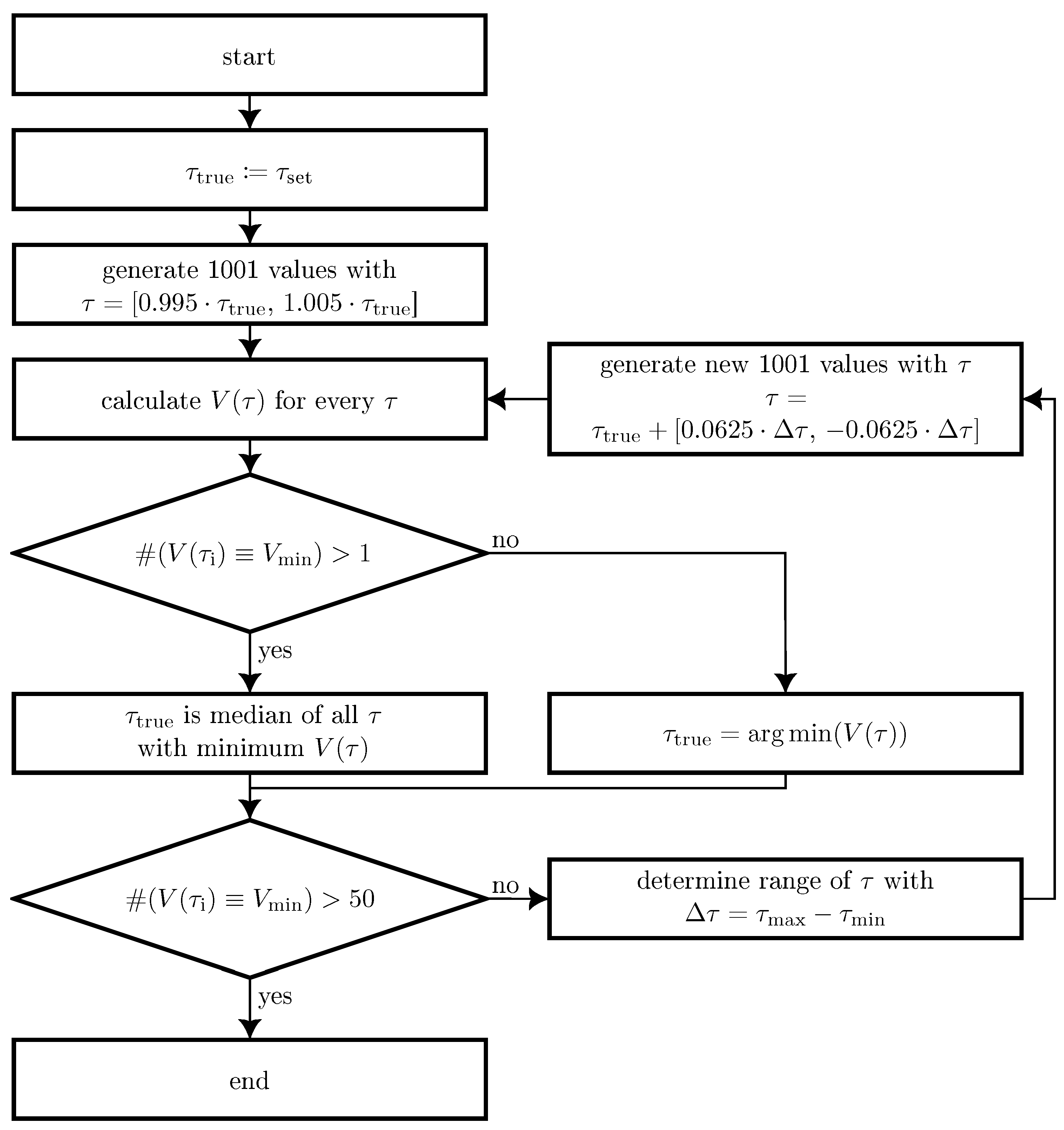
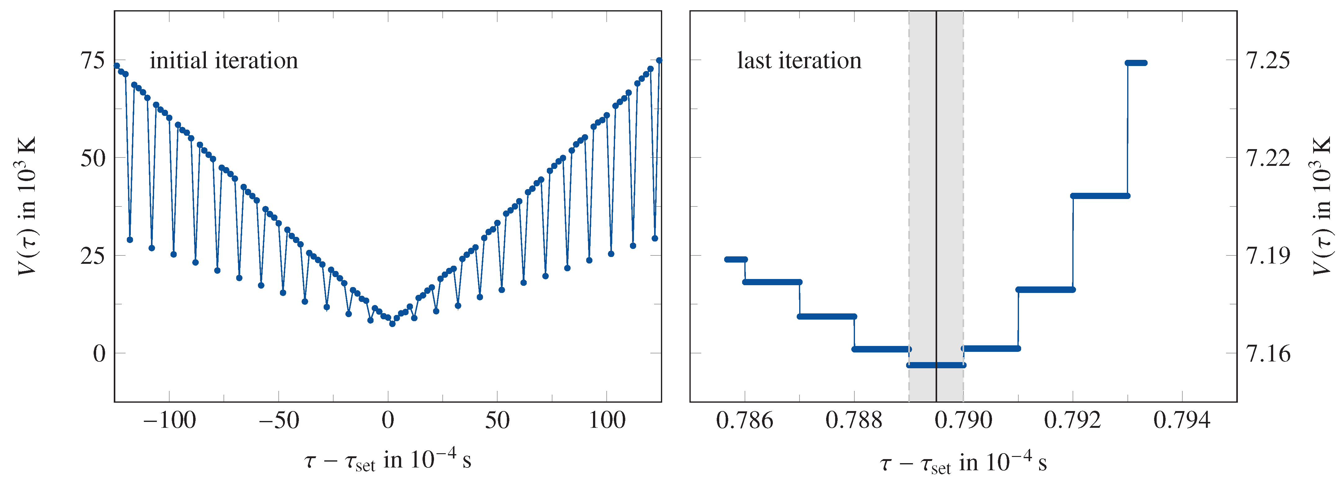
2.2. Period Estimation

The aforementioned experimental procedure comprises two independent periods: $\Delta t_{\mathrm{s}}$ and ${\tau }_{\mathrm{set}}$. Depending on the experimental setup, this poses additional challenges. If both periods are not linked to a common fundamental clock, the actual values might differ from the expected ones. Although this difference may be small in absolute terms, it results in a significant deviation for longer time scales.

One approach is to consider the period of the signal, ${\tau }_{\mathrm{set}}$, as not exact and to construct it from the data themselves. The algorithm described in the following text is based on the work by Rader [15]. When using a non-exact value for ${\tau }_{\mathrm{set}}$, the collapsing procedure (1) results in an increasing misalignment of the thermal transients, which appears as high-frequency noise in the reconstructed signal. Assuming that the correct signal period, ${\tau }_{\mathrm{true}}$, results in the curve with the lowest noise, the uncertainty in the signal can be quantified by the cost function:

$$V\left(\tau \right)=\sum _i\left|T\left(t_i^{\prime }\right)-T\left(t_{i+1}^{\prime }\right)\right|.$$

(3)

Here, all temperature differences between two neighboring data points are accumulated. When two thermal transients have a sufficiently large relative offset in time, the relative ordering of the data points changes in the collapsed time series. Consequently, the nearest neighbor changes and with it $V\left(\tau \right)$. A simplified Rader algorithm is applied; a flow chart is shown in Figure 2. The search for the true value of the sampling period, ${\tau }_{\mathrm{true}}$, begins in the interval ${\tau }_{\mathrm{set}}\pm 0.005·{\tau }_{\mathrm{set}}$. A total of 1001 evenly distributed trials for the sampling period, ${\tau }_{\mathrm{set}}$, within this range are selected. For these periods, the cost function (3) is calculated. Next, the trial period with the minimum cost function is set as the next best guess for the true value, ${\tau }_{\mathrm{true}}$. If there are multiple trial periods with the same minimum error, a median of these periods is used as the new ${\tau }_{\mathrm{true}}$. Subsequently, 1001 trial periods in the range ${\tau }_{\mathrm{true}}\pm 0.0625·\Delta \tau$ are chosen and the previous steps are repeated. $\Delta \tau$ is the difference between the largest trial period and the smallest trial period, $\tau$, of the previous iteration. The iteration is stopped if more than 50 trial periods have the same cost value, or if a set number of iterations has been reached. Depending on the application, the termination parameters and interval sizes can be adjusted.

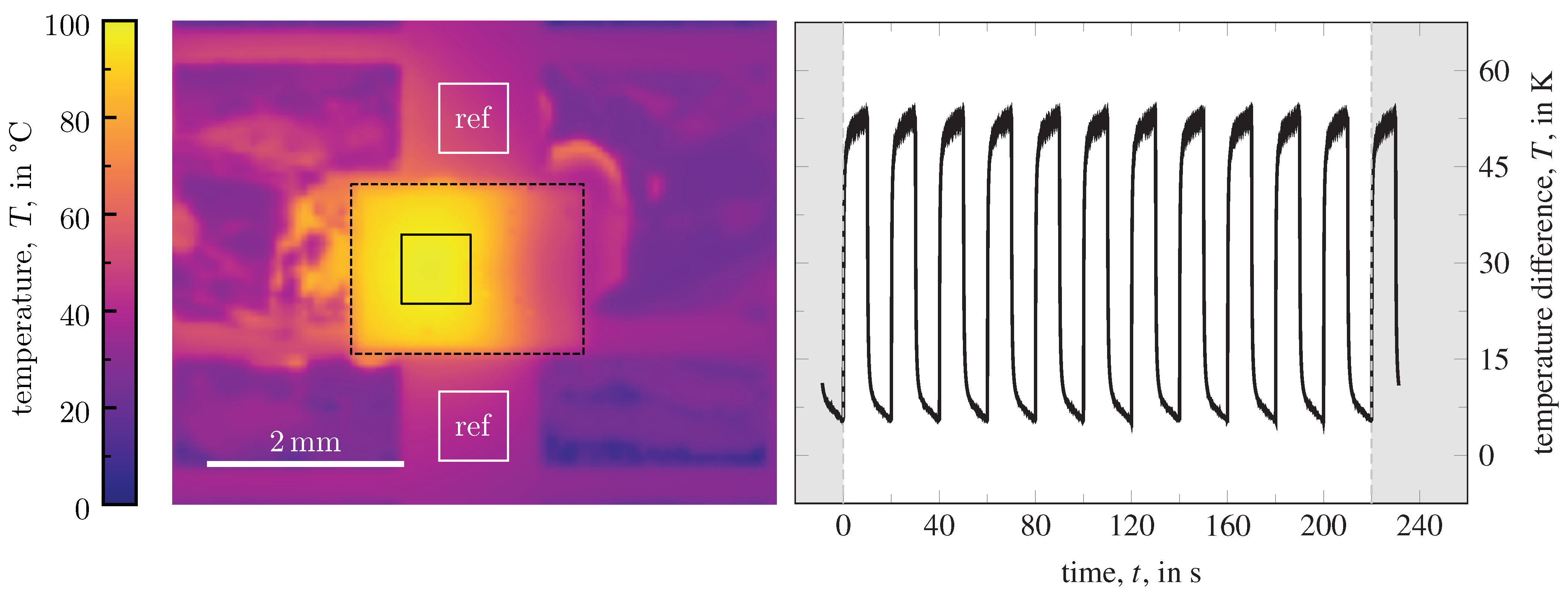
3. Experimental Setup

As a proof of concept, the thermal transient and impedance of a surface-mounted device (SMD) diode (Vishay DO-219AD) soldered to an FR-4 printed circuit board was analyzed by super-frequency sampling. Figure 3 shows a sketch of the experimental setup. The board is directly screwed to an aluminum base plate. The heating current, supplied by a programmable power supply (Hameg HMP4040), is switched by an n-channel power MOSFET (Fairchild BUZ11_NR4941), which is controlled by a frequency generator (Hameg HMF2550). To determine the ohmic loss, the voltage drop across the diode is measured by a voltmeter (Keithley 2700) in a 4-wire configuration.

The surface temperature of the diode is measured by a thermography system with an InSb focal plane array (InfraTec GmbH, Dresden, Germany, ImageIR® 8380S). The thermographic camera has a full-frame resolution of $640\times 512$ pixels with a sampling rate of 200 $\mathrm{Hz}$. When using the quad-frame setting ($160\times 128$ pixels), the sampling rate increases to 1000 $\mathrm{Hz}$. For a sufficient resolution of a thermal transient, the sampling period must be 10 to 15 times smaller than the smallest time constant of the response [11]. For semiconductor components, typical time constants are greater than one millisecond. Consequently, the target sampling rate is approximately 100 μs, and thus, a speed-up factor of $N=10$ is required. The modulation frequency is set to ${\tau }_{\mathrm{set}}=20 \mathrm{s}+1·{10}^{-4} \mathrm{s}$. The applied current is set to $0.9$ $\mathrm{A}$ with a duty cycle of 50%. The resulting voltage drop across the diode is found to be in the range between $0.983$ $\mathrm{V}$ and $1.017$ $\mathrm{V}$. To measure the system in a quasi equilibrium state, the periodic excitation is started a few minutes prior to the temperature recording.

4. Results and Discussion

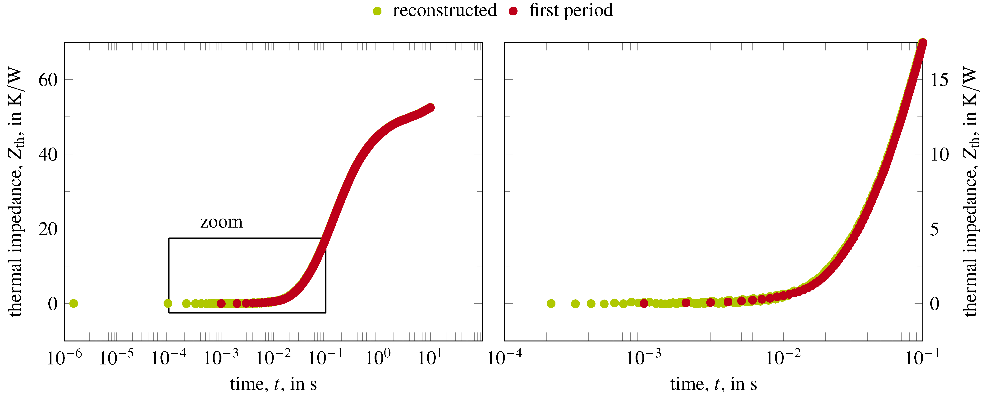
4.1. Thermal Transient Reconstruction

The above-described setup is used to measure the thermographic image of an SMD diode, as shown in Figure 4 (left). The diode with the dimensions of $2.3$ mm by $1.4$ $\mathrm{m}$$\mathrm{m}$ is indicated by a dashed line. The algorithm is evaluated based on the temperature difference between the mean of the $11\times 11$ test area on top of the diode (black square) and the mean temperature of the two reference areas, which also have $11\times 11$ pixels in size (white squares). Figure 4 (right) shows the temporal behavior of the temperature difference for the test area, with the diode excited by a square wave signal. The true sampling period, ${\tau }_{\mathrm{true}}$, is then extracted from the measurement data in the temporal range from 0 s to 220 s, as described in Section 2.2.

Figure 5 shows the cost function for the initial (left) and for the final search range (right). In the first iteration, the cost function oscillates between two branches but converges to a clear minimum. The refinement of the search interval, ${\tau }_{\min }\dots {\tau }_{\max }$, results in the formation of plateaus, as shown in Figure 5 (right). Transitions between these plateaus occur at critical periods at which the sequence of the reconstructed measurement points changes. Within the plateaus, only the distance between the points varies, which has no impact on the cost function. The algorithm converges in this example in seven iterations, resulting in a true period value of ${\tau }_{\mathrm{true}}=20 \mathrm{s}+1.7895·{10}^{-4} \mathrm{s}$ with an uncertainty of $\Delta {\tau }_{\mathrm{true}}=0.0005·{10}^{-4} \mathrm{s}$. The uncertainty is given by the width of the plateau (indicated as the gray shaded area).

Having extracted the true period, ${\tau }_{\mathrm{true}}$, the recorded thermal transient (Figure 4 Right) is collapsed. The starting (end) point of the heating curves is defined as the first significant increase (decrease) in temperature. The impedance, $Z_{\mathrm{th}}\left(t\right)$, is then calculated via

$$Z_{\mathrm{th}}\left(t\right)={\displaystyle \frac{T\left(t\right)-T_0}{P}}.$$

(4)

The initial temperature, $T_0$, of the heating (cooling) is equal to the end temperature of the cooling (heating) curve. The power amounts to $P=0.9 \mathrm{A}·1 \mathrm{V}=0.9 \mathrm{W}$.

The calculated thermal impedance of the heating phase is shown in Figure 6. The points, derived from an analysis of the first period only, are depicted as red dots. With super-frequency sampling (eleven periods), however, additional points (green) within each decade are obtained. The temporal resolution is increased and allows for the analysis of the thermal behavior in the range between ${10}^{-4}$ and ${10}^{-3}$.

4.2. Speed-Up Factor

From here on, only the first 10 periods are examined to achieve the desired speed-up factor of 10, as this should be sufficient. For an analysis of the temporal resolution of the reconstructed signal, the reconstructed sampling period, $\Delta t_{\mathrm{r},i}=t_{i+1}^{\prime }-t_i^{\prime }$, is calculated for all data points.

In practice, these $\Delta t_{\mathrm{r},i}$ follow a distribution with the center of the distribution situated at a value very close to $1·{10}^{-4}$. This is due to the fact that the total time and total number of points are well-defined. The width of the distribution depends on the accuracy of the relative frequencies. In the following text, a typical and worst-case evaluation for the speed-up factor is performed based on the above measurement. In the event of a larger reconstructed sampling period falling into a moment of particular relevance, the aforementioned worst-case scenario manifests itself.

A histogram of the reconstructed sampling periods with the median, $\Delta {\tilde{t}}_{\mathrm{r}}$, and the 95th-quantile, $Q_{0.95}$, (i.e., the slowest 5% of the sampling periods) is shown in Figure 7 (left). The relationship between the reconstructed sampling period, $\Delta t_{\mathrm{r}}$, and the speed-up factor, N, is given by (2) with $\Delta t_{\mathrm{r}}=\Delta t_{\mathrm{s}}/N$. The speed-up factor of the sampling frequency is, thus, given by

$$\begin{array}{c}\hfill N_{\Delta {\tilde{t}}_{\mathrm{r}}}={\displaystyle \frac{\Delta t_{\mathrm{s}}}{\Delta {\tilde{t}}_{\mathrm{r}}}}={\displaystyle \frac{{10}^{-3} \mathrm{s}}{0.98·{10}^{-4} \mathrm{s}}}=10.2,N_{Q_{0.95}}={\displaystyle \frac{\Delta t_{\mathrm{s}}}{Q_{0.95}}}={\displaystyle \frac{{10}^{-3} \mathrm{s}}{1.2·{10}^{-4} \mathrm{s}}}=8.5.\end{array}$$

(5)

In a subsequent step, the cumulative distribution of the reconstructed sampling period, $\Delta t_{\mathrm{r}}$, is calculated for a different number of periods. Figure 7 (right) shows the result. Curve “1” represents the result when the first period is used only (see Figure 6). Here, only the sampling period of the camera with a frequency of $1/1000\mathrm{Hz}$ is present as no reconstruction is performed yet. With each additional period included in the calculation, the relative contribution of the reconstructed sampling periods with a temporal resolution larger than ${10}^{-4} \mathrm{s}$ decreases. For five periods (lime curve), their relative contribution amounts to 80%. For ten periods, the mean sampling period of the reconstructed signal is $1.0004·{10}^{-4} \mathrm{s}$. This value is very close to the desired sampling period of $1·{10}^{-4} \mathrm{s}$. An increase to eleven periods does not result in a further improvement in the overall temporal resolution as only periods below $1·{10}^{-4} \mathrm{s}$ are added.

4.3. Overall Validity

The $11\times 11$ area in the center of the diode is chosen rather arbitrarily as it seems that the temperature distribution in this area is quite homogeneous (Figure 4, left). To investigate the influence of the area’s size on the quality of the result, the analysis is repeated for all possible sub-areas within the $11\times 11$ area, i.e., in total 121 ($1\times 1$) areas, 100 ($2\times 2$) areas, 81 ($3\times 3$) areas, 64 ($4\times 4$) areas, 49 ($5\times 5$) areas, 36 ($6\times 6$) areas, 25 ($7\times 7$) areas, 16 ($8\times 8$) areas, 9 ($9\times 9$) areas, 4 ($10\times 10$) areas, and 1 ($11\times 11$) area, with each of these 506 test areas having a different ${\tau }_{\mathrm{true}}-{\tau }_{\mathrm{set}}$. The cumulative distribution of these ${\tau }_{\mathrm{true}}-{\tau }_{\mathrm{set}}$, grouped by the area’s size, is shown in Figure 8 (left). It can be observed, for instance, that for the $1\times 1$ sized areas, approximately 40% of the sampling periods have the same value as the period of the single $11\times 11$ area. For areas equal or larger than $8\times 8$, the algorithm converges to the same value. It should be noted that, in all cases, the true sampling period, ${\tau }_{\mathrm{true}}$, is larger than the set sampling period, ${\tau }_{\mathrm{set}}=20 \mathrm{s}+$$1·{10}^{-4} \mathrm{s}$. This indicates that the internal clock of the signal generator is $3.9·{10}^{-4} \mathrm{s}$ slower than that of the camera system.

Figure 8 (right) shows the cumulative distribution of the medians, $\Delta {\tilde{t}}_{\mathrm{r}}$, for the different area’s sizes. For some cases, the $\Delta {\tilde{t}}_{\mathrm{r}}$ are smaller than $0.1·{10}^{-4} \mathrm{s}$. In these cases, the reconstructed points for one period are very close to each other and followed by a larger gap. This indicates that the reconstructed points are very unevenly distributed as the algorithm minimizes the difference of the temperature values of consecutive data points without considering their temporal difference.

To measure the influence of noise on the sample period reconstruction, the signal-to-noise ratio (SNR) is calculated for each sub-area. The signals are filtered with a first-order Savitzky–Golay filter. Figure 9 illustrates the average SNR, which is given by the average of all corresponding sub-area SNRs. The error bar indicates the range between the 5th and the 95th percentiles, $Q_{0.05}$ and $Q_{0.95}$, of the signal-to-noise ratios of the input signals. For the $8\times 8$ area, the reconstructions of all $8\times 8$ sub-areas converge to the same sampling period, ${\tau }_{\mathrm{true}}$. The average SNR of the $8\times 8$ area amounts to 5680. This threshold is indicated by the dashed line.

5. Conclusions

The enhancement of temporal resolution in thermographic transient measurements by super-frequency sampling represents a significant improvement for thermographic analysis. This technique enables a more detailed analysis of thermal transients due to an increased sampling density. An analysis of the thermal transients of a periodically switched SMD test diode shows an increase in sampling frequency by a factor of 10. While the sampling frequency of the infrared camera system in use was limited to 1 kHz, the sampling frequency could be increased to 10 kHz, i. e., a temporal resolution of 100 ms.

The limitation of this algorithm is its long measurement time, which makes it important to consider a possible slow thermal drift of the measurement setup. To minimize the influence of thermal drift, the measurement environment should be well insulated from external thermal influences. Furthermore, long measurement times can lead to a large amount of infrared data, which can be computationally demanding to handle. These effects as well as the temporal accuracy of the measurement device limit the practically achievable speed-up factors.

The benefit of super-frequency sampling is of particular importance in the field of power-electronics and other small components. (i) High-frequency sampling in the infrared spectral range enables the monitoring of fast thermal transitions with increased clarity. An enhanced temporal resolution at full spatial resolution is of particular importance for the identification of hot spots and thermal gradients, yielding a better approach for thermal management strategies. (ii) Super-frequency sampling is also useful for the validation of computational fluid dynamics (CFD) simulations. By providing empirical data that closely match the high-resolution temporal dynamics of thermal processes, super-frequency sampling enables the fine-tuning of CFD models, ensuring that simulations more accurately reflect real-world conditions. This synergy enhances predictive capabilities, allowing for more precise design optimizations and validations before physical prototypes are tested. (iii) The early detection of potential thermal issues, made possible through a detailed analysis, allows engineers to implement design and testing phase adjustments. Such proactive measures are critical in applications where high-power densities are prevalent, such as vehicle electrification and aerospace, ensuring that the reliability and performance of power electronics are optimized.

References

1. Mayer, Z.; Epperlein, A.; Vollmer, E.; Volk, R.; Schultmann, F. Investigating the Quality of UAV-Based Images for the Thermographic Analysis of Buildings. Remote Sens. 2023, 15, 301. [Google Scholar] [CrossRef]
2. Magalhaes, C.; Mendes, J.; Vardasca, R. Meta-Analysis and Systematic Review of the Application of Machine Learning Classifiers in Biomedical Applications of Infrared Thermography. Appl. Sci. 2021, 11, 842. [Google Scholar] [CrossRef]
3. Panahandeh, S.; May, D.; Wargulski, D.; Boschman, E.; Schacht, R.; Ras, M.A.; Wunderle, B. Infrared thermal imaging as inline quality assessment tool. In Proceedings of the 22nd International Conference on Thermal, Mechanical and Multi-Physics Simulation and Experiments in Microelectronics and Microsystems (EuroSimE), St. Julian, Malta, 19–21 April 2021; pp. 1–6. [Google Scholar] [CrossRef]
4. Jahn, N.; Pfost, M. Size Determination of Voids in the Soldering of Automotive DC/DC-Converters via IR Thermography. In Proceedings of the 21st IEEE Intersociety Conference on Thermal and Thermomechanical Phenomena in Electronic Systems (iTherm), San Diego, CA, USA, 31 May–3 June 2022; pp. 1–7. [Google Scholar] [CrossRef]
5. Vavilov, V.; Burleigh, D. Infrared Thermography and Thermal Nondestructive Testing, 1st ed.; Springer: Cham, Switzerland, 2020. [Google Scholar] [CrossRef]
6. Ibarra-Castanedo, C.; Maldague, X.P. Defect depth retrieval from pulsed phase thermographic data on Plexiglas and aluminum samples. In Thermosense XXVI; Burleigh, D.D., Cramer, K.E., Peacock, G.R., Eds.; International Society for Optics and Photonics; SPIE: Bellingham, WA, USA, 2004; Volume 5405, pp. 348–356. [Google Scholar] [CrossRef]
7. Galmiche, F.; Leclerc, M.; Maldague, X.P. Time aliasing problem in pulsed-phased thermography. In Thermosense XXIII; Rozlosnik, A.E., Dinwiddie, R.B., Eds.; International Society for Optics and Photonics; SPIE: Bellingham, WA, USA, 2001; Volume 4360, pp. 550–553. [Google Scholar] [CrossRef]
8. Bagnoli, P.; Casarosa, C.; Ciampi, M.; Dallago, E. Thermal resistance analysis by induced transient (TRAIT) method for power electronic devices thermal characterization. I. Fundamentals and theory. IEEE Trans. Power Electron. 1998, 13, 1208–1219. [Google Scholar] [CrossRef]
9. Ziegeler, N.J.; Nolte, P.W.; Schweizer, S. Thermographic network identification for transient thermal heat path analysis. Quant. Infrared Thermogr. J. 2022, 20, 93–105. [Google Scholar] [CrossRef]
10. Nichia Corporation. 16,384 LEDs to Revolutionize Automotive Lighting: Nichia and Infineon Launch Industry’s First High-Definition Micro-LED Matrix Solution. Available online: https://www.nichia.co.jp/en/newsroom/2023/2023_011901.html (accessed on 26 March 2024).
11. Ezzahri, Y.; Shakouri, A. Application of network identification by deconvolution method to the thermal analysis of the pump-probe transient thermoreflectance signal. Rev. Sci. Instrum. 2009, 80, 074903. [Google Scholar] [CrossRef] [PubMed]
12. Rupniewski, M.W. Reconstruction of Periodic Signals From Asynchronous Trains of Samples. IEEE Signal Process. Lett. 2021, 28, 289–293. [Google Scholar] [CrossRef]
13. Vandewalle, P.; Sbaiz, L.; Vandewalle, J.; Vetterli, M. Super-Resolution From Unregistered and Totally Aliased Signals Using Subspace Methods. IEEE Trans. Signal Process. 2007, 55, 3687–3703. [Google Scholar] [CrossRef]
14. Tao, R.; Li, B.Z.; Wang, Y. Spectral Analysis and Reconstruction for Periodic Nonuniformly Sampled Signals in Fractional Fourier Domain. IEEE Trans. Signal Process. 2007, 55, 3541–3547. [Google Scholar] [CrossRef]
15. Rader, C. Recovery of undersampled periodic waveforms. IEEE Trans. Acoust. Speech Signal Process. 1977, 25, 242–249. [Google Scholar] [CrossRef]
16. Schmid, M.; Bhogaraju, S.K.; Hanss, A.; Elger, G. A New Noise-Suppression Algorithm for Transient Thermal Analysis in Semiconductors Over Pulse Superposition. IEEE Trans. Instrum. Meas. 2021, 70, 6500409. [Google Scholar] [CrossRef]
17. Pradere, C.; Clerjaud, L.; Batsale, J.C.; Dilhaire, S. High speed heterodyne infrared thermography applied to thermal diffusivity identification. Rev. Sci. Instrum. 2011, 82, 054901. [Google Scholar] [CrossRef] [PubMed]
Figure 1. Example of a thermal transient measured with super frequency sampling: signal as-measured (left) and reconstructed after collapsing the time series (right).
Applsci 14 07635 g001
Figure 2. Flow chart to determine the true period, τ true , that minimizes the cost function V ( τ ) .
Applsci 14 07635 g002
Figure 3. Sketch of the experimental setup. The heating current from the power supply is switched by a MOSFET, which is controlled by a frequency generator. A voltmeter is used for voltage measurements.
Applsci 14 07635 g003
Figure 4. (left) Thermographic image of the diode in the on-state. The marked areas indicate the 11 × 11 test area as well as the two 11 × 11 reference areas. (right) Temporal behavior between the mean temperature difference of the test area at the center of the diode and the two reference areas.
Applsci 14 07635 g004
Figure 5. Cost function for the reconstructed temperature signal. (left) Initial search range. (right) Final search range with a global minimum in the gray range and the obtained true sampling value, τ true , marked with a solid black line. On the x-axis, the difference between the used signal period for the reconstruction, τ , and the set signal period, τ set , is shown.
Applsci 14 07635 g005
Figure 6. Comparison of the thermal impedance in the first period and the reconstructed values.
Applsci 14 07635 g006
Figure 7. (left) Histogram of sampling periods within the reconstructed signal (on the basis of ten periods). (right) Cumulative distribution of the reconstructed sampling periods for a different number of periods included in the analysis.
Applsci 14 07635 g007
Figure 8. (left) Cumulative distribution of the true sampling periods, τ true , obtained for all 506 possible test areas on top of the diode (Figure 4 (left)). (right) Cumulative distribution of the medians of the reconstructed sampling periods, Δ t ˜ r .
Applsci 14 07635 g008
Figure 9. Average signal-to-noise ratio, SNR ¯ , of the different N × N test areas. The error bar indicates the range between the 5th and the 95th percentiles, Q 0.05 and Q 0.95 , of the signal-to-noise ratios of the input signals. The average signal-to-noise ratio, for which all sub-areas converge to the same sampling period, τ true , is indicated by the dashed line.
Applsci 14 07635 g009
Disclaimer/Publisher’s Note: The statements, opinions and data contained in all publications are solely those of the individual author(s) and contributor(s) and not of MDPI and/or the editor(s). MDPI and/or the editor(s) disclaim responsibility for any injury to people or property resulting from any ideas, methods, instructions or products referred to in the content.