A Carbon Benefits-Based Signal Control Method in a Connected Environment

Abstract

This study proposes an innovative carbon benefits-based signal control method for connected vehicle (CV) environments, aiming to reduce carbon emissions at urban intersections. By integrating a Carbon Inclusion Mechanism (CIM), the proposed approach offers carbon rewards to vehicles adhering to speed guidance. The method exhibits the following features: (i) higher ceiling of carbon emissions reduction at signal control intersection; (ii) higher compliance rate (CR) of vehicles by taking advantage of carbon economic incentives; (iii) a method for calculating carbon emissions reduction at the intersection. To validate the effectiveness, performance evaluations of emissions, stop frequencies, and delays were conducted through microscopic simulation. Sensitivity analysis encompassed various traffic demands, different CRs of carbon-benefit connected vehicles (CBCVs), and unbalanced traffic demand. The results demonstrated that the proposed method excels in reducing traffic emissions, stop frequencies, and delays. Specifically, carbon emissions were reduced by 5.24% to 17.60%, stop frequencies decreased by 14.8% to 75.4%, and delays were reduced by 22.82% to 52.62%. By utilizing connected vehicle technology and CIM, this study contributes to sustainable urban traffic management, laying a foundation for future research and the practical implementation of emission reduction strategies.

1. Introduction

Greenhouse gas emissions pose a global challenge. According to the International Energy Agency (IEA) [1], the transport sector is responsible for 25–30% of a country’s total carbon emissions. Within the transportation system, road transport contributes approximately 80% of emissions and energy consumption, with passenger cars responsible for 66.3% of road transport emissions, predominantly on urban roads. Given that exhaust emissions from passenger cars on urban roads are directly released into living areas, they have a significant impact on public health and travel experience, creating an urgent need for emission reduction.

Signal-controlled intersections are fundamental components of urban roads and critical scenarios for urban road emission reduction in urban roads. When vehicles pass through signal-controlled intersections, some must come to a complete stop at red lights. During this process, vehicles undergo sequential conditions of deceleration, idling, and acceleration. Evaluations using microscopic simulation models show that the stopping conditions lead to additional emissions [2,3]. Particularly during the start-up acceleration phase after a stop, vehicles emit a significant amount of pollutants [4,5]. To address this issue, many studies [6,7,8,9,10,11,12] have developed adaptive signal control methods aimed at reducing vehicle stops as much as possible to improve carbon emissions at intersections. These methods optimize the allocation of green light durations at intersections based on the number of vehicles arriving from each direction. The number of arrival vehicles is predicted based on data collected from upstream detectors. However, these methods exhibit limitations in practical application due to their reliance on the assumption that all vehicles travel at a predefined speed. In reality, drivers cannot always achieve this predefined speed. Variations in driving behavior and individual differences result in fluctuations in actual vehicle speeds. For example, conservative drivers may drive slower than the predefined speed and miss the green light phase at intersections. In contrast, aggressive drivers may drive faster and arrive too early, resulting in additional stops and increased emissions. Indeed, the challenges faced by adaptive signal control methods stem from the uncertainty of vehicle arrival times. To overcome these limitations, it is critical to enhance the optimization of signal control methods by introducing vehicle speed guidance [13].

With the maturation of wireless communication, connected vehicles (CVs) have emerged. CVs can use Vehicle-to-Infrastructure (V2I) communication to transmit driver information to the signal control center. This information includes departure points, destinations, and precise trajectory data, such as per-second speed and position. Additionally, CVs can receive intersection signal plans in advance and adjust their speeds accordingly [14,15,16]. This reduces the impact of unpredictable vehicle arrivals on control systems, helping to avoid stops at intersections during red lights. Consequently, it further contributes to the reduction in carbon emissions [17,18,19,20]. Numerous studies [21,22,23,24,25,26,27,28,29] have developed eco-friendly coordinated signal control with vehicle speed guidance. These methods provide second-by-second speed planning for vehicles, ensuring that vehicles arrive at intersections in alignment with green phases, maximizing the number of vehicles passing through and reducing stops. However, most of these studies assume that vehicles possess autonomous driving capabilities, enabling a precise execution of speed guidance commands. This assumption is unrealistic in the near future, as it is projected that Connected and Autonomous Vehicles (CAVs) will not achieve a 100% market penetration rate (MPR) by the 2060s [30]. Consequently, in the short term, the practical implementation of these methods remains challenging. Vehicles lacking autonomous driving functionality may struggle to adhere to speed guidance, resulting in low compliance rates (CRs) and potentially diminishing the benefits of coordinating with signal plans. Therefore, it is critical to enhance the CR of vehicles by following speed guidance.

With significant international attention focused on promoting public low-carbon actions, many countries are seeking measures to influence and encourage people to participate in reducing carbon emissions. The IPCC Sixth Assessment Report indicates that changing people’s behaviors could reduce carbon emissions by 40–70% by 2050 [31]. To achieve this goal, China has proposed the Carbon Inclusion Mechanism (CIM). CIM facilitates the exchange of green behavior data among the public, enterprises, and the government [32]. By establishing personal green assets and green credits, the carbon reduction benefits generated by individual low-carbon behaviors can be acquired by enterprises in need. This transforms individual low-carbon actions from purely altruistic behaviors into rewardable actions, significantly increasing the likelihood of individuals choosing low-carbon behaviors.

On a theoretical level, scholars [33] have demonstrated the potential of CIM to synergize with intelligent transportation system (ITS), advocating it as a feasible pathway for optimizing transportation structures, promoting shifts in travel modes, and ultimately achieving emission reductions in the transportation sector [34]. Empirical research has also confirmed CIM’s significant effectiveness in promoting green tourism [35,36,37]. For example, in Beijing, the “Personal Carbon Ledger” project has successfully encouraged over 88 million emission reduction actions, resulting in approximately 40,000 tons of carbon reductions [38]. This demonstrates that CIM measures have the potential to enhance public participation in green behaviors. Inspired by these theoretical and practical insights, we propose that CIM can effectively improve vehicle compliance with target speeds. Adhering to eco-speed guidance strategies recommended by signal control systems is essentially practicing green, low-carbon driving behavior. In a connected environment, the emission reduction benefits of such behaviors can be quantified by the control center. The obtained emission reduction benefits can be used for carbon trading, with the transaction price serving as a carbon reward for the vehicle’s green behavior. This integration of CIM with traffic control strategies can incentivize vehicles to comply with speed guidance. However, there is a notable lack of exploration in combining CIM with traffic signal control methods. Therefore, developing and integrating CIM to enhance signal control methods for reducing emissions is urgently needed.

Given the research gap in the existing methods, this paper proposes an enhanced signal control method in a connected environment. It has the following features:

• Higher ceiling of carbon emissions reduction at signal control intersection;
• Ensured higher CR of vehicles by taking advantage of carbon economic incentives;
• Provided a method for calculating carbon emissions reduction at the intersection.

This paper is organized as follows: Section 2 presents the control mechanism. Section 3 presents the problem description. Section 4 presents the methodology. Section 5 evaluates the performance of the proposed method. Section 6 provides the conclusions.

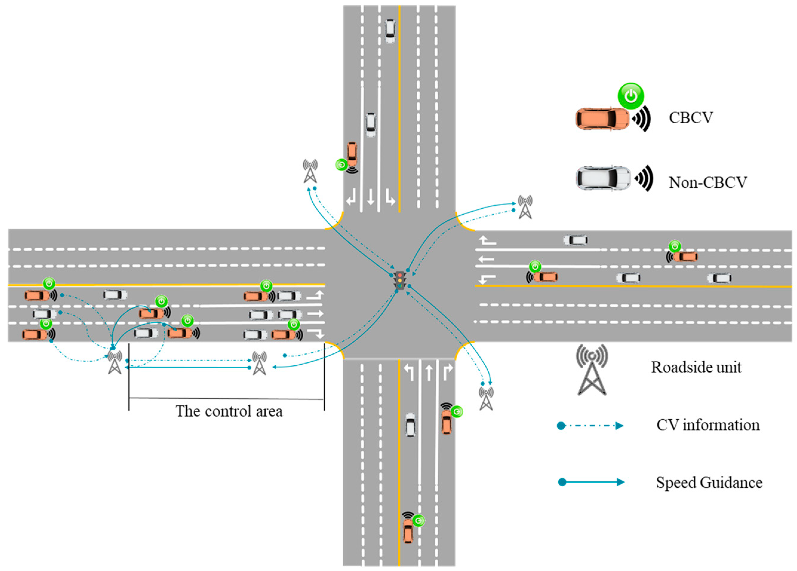
2. Control Mechanism

This section provides the rationale for how the features are achieved.

Higher ceiling of carbon emissions reduction at signal control intersection: The carbon emissions reduction is achieved by the coordinated optimization of signal control and vehicle speed guidance. The optimization of signal control aims to minimize vehicle speed fluctuations within intersection areas, as higher speed fluctuations result in increased emissions. The optimization of signal timing will determine the optimal allocation of green time for each phase. The optimization of vehicle speed guidance aims to track the green time phases provided by signal control, designing optimal speed recommendations for vehicles so that the maximum number of vehicles can pass through during the green phase. This approach reduces the frequency of vehicle stops and starts, lowering carbon emissions. This coordinated optimization could significantly enhance carbon emission reduction.

Ensured higher compliance rate of vehicles by taking advantage of carbon economic incentives: To enhance vehicle compliance, this research proposes a CIM integrated with signal control. Before entering the control area, CVs can preview the estimated carbon reward value for the current intersection, which is based on the actual reward amounts distributed to vehicles in the previous period. By demonstrating potential economic benefits, drivers can be encouraged to follow speed guidance. CVs that follow the speed guidance become carbon-benefit connected vehicles (CBCVs). The control center would monitor the driving behavior of CBCVs within the control area to determine their economic rewards. The level of compliance with speed guidance directly influences their carbon rewards, further incentivizing effective adherence to speed guidance.

Provided a method for calculating carbon emissions reduction at intersection: To accurately assess the carbon reduction benefits of CBCVs executing speed guidance strategies, this study proposes a comprehensive evaluation method. The method calculated the emission reduction benefits from two aspects. The first aspect is the direct emission reduction benefit of CBCVs. This assessment is based on the difference in emissions between scenarios where a CBCV receives guidance and scenarios where it does not, quantifying the reduction in emissions as the benefit. The second part evaluates the indirect carbon reduction benefits of CBCVs. This involves proposing a grouping strategy to determine the non-CBCV group influenced by CBCV guidance. The emission difference of this group before and after being influenced by CBCV guidance is calculated as the reduction benefit. All emission calculations are based on a microscopic emission calculation model, ensuring the accuracy of the computations.

3. Problem Statements

The studied scenario is an isolated signalized intersection, as depicted in Figure 1. It highlights the application scope of the proposed method. The scenario is a typical four-leg, three-lane (in each direction) signalized intersection. These three lanes have different uses: a left-turn lane, a straight-through lane, and a right-turn lane. The signal plan has a fixed number of phases and execution order. Each phase is divided into an effective green interval and a clearance time (including yellow and all-red times). The clearance time is pre-designed and fixed within the system. The proposed method optimizes the start and end times of each phase during the optimization process. The maximum and minimum green times are in line with standard signal design practices.

In this study, the scenario operates within a connected traffic environment. In this context, all vehicles can communicate in real time with roadside units through V2V and V2I technologies. The roadside control center can obtain real-time vehicle status information (position, speed). The control area extends from the upstream section to the location before the stop line, which is selected as 300 m in this study. Within the control area, the lane-changing behavior of vehicles is not considered. The control center provides the required speed commands to CBCVs at an update frequency of $N_{sg}∆t$.

4. Methodology

This section provides a detailed representation of the proposed method, including parameters and notations, control structure, model formulation, and solution method.

4.1. Parameters and Notations

The notations and parameters utilized hereafter are defined in

Table 1. Notations and parameters.

Notations	Explanation	Unit
TD	The total delay at the intersection	s
Y	The signal timing plan
K	The set of all phases
${\mathit{\Omega }}^{\mathit{k}}$	The vehicles set within the control area of phase k
${\mathit{\Omega }}^{{\mathit{k}}^{\mathit{c}}}$	The vehicles set based on CBCVs grouping within the control area of phase k
$k$	The phase number
${\omega }_k$	The vehicle number, indicating the ωk-th vehicle in phase k
${\omega }_k^c$	The number of CBCVs in the direction of phase k
$D_{{\omega }_k}$	The delay of vehicle ωk during passing through the intersection	s
$u_k^i$	The start time of the i-th green time for phase k
$o_k^i$	The end time of the i-th green time for phase k
$N$	The number of optimization cycles
$x^{{\omega }_k}$	The distance between vehicle ${\omega }_k$ and the stop line	m
$∆t$	The planning time interval.	s
$t_0$	The start time of the control algorithm.
$h_{{\omega }_k}$	The time when vehicle ${\omega }_k$ crosses the stop line in trajectory planning	s
$t_c^{{\omega }_k}$	The time when the vehicle ${\omega }_k$ passes the stop line under signal control	s
$t_a^{{\omega }_k}$	The time taken by the vehicle ${\omega }_k$ to accelerate from crossing the stop line to its desired speed	s
$t_{free}^{{\omega }_k}$	The time the vehicle spends in free flow to reach the point where it achieves $t_a^{{\omega }_k}$	s
$v_c$	The speed of the vehicle as it crosses the stop line	m/s
$v_l$	The speed limit on the road	m/s
$L$	The length of the control area	m
$t_{clear}$	The clearance time required during phase switching	s
$g_{min}$	The minimum green time duration	s
$g_{max}$	The maximum green time duration	s
${\tau }_{\omega }$	Execution cycle of the rolling horizon scheme	s
${\tau }_n$	The safety interval in the rolling horizon scheme	s
$\alpha$	The weight of the stop time
${\Omega }_{{\omega }_k^c}^{k^c}$	$\mathrm{The} \mathrm{set} \mathrm{of} \mathrm{vehicles} \mathrm{guided} \mathrm{by} \mathrm{CBCVs} {\omega }_k^c$
${\tau }_{cf}$	Time lag in the Newswell model	s
$d_{cf}$	Spatial lag in the Newswell model	m
$N_{sg}∆t$	The transmission interval for speed instructions	$\mathrm{g}$
$a_L^{{\omega }_k}$	Maximum deceleration of the vehicle	m/s2
$a_U^{{\omega }_k}$	Maximum acceleration of the vehicle	m/s2
$v_{sg}^{{\omega }_k^c}\left(t\right)$	$\mathrm{The} \mathrm{set} \mathrm{of} \mathrm{target} \mathrm{speed} \mathrm{for} \mathrm{vehicle} {\omega }_k^c$	m/s
$v_{at}^{{\omega }_k^c}\left(t\right)$	$\mathrm{The} \mathrm{set} \mathrm{of} \mathrm{actual} \mathrm{speed} \mathrm{of} \mathrm{vehicle} {\omega }_k^c$
$TH$	The threshold for judging whether the vehicle has complied with the speed guidance.
$R\left({\omega }_k^c\right)$	$\mathrm{The} \mathrm{carbon} \mathrm{reward} \mathrm{amount} \mathrm{allocated} \mathrm{to} {\omega }_k^c$
$CE\left({\omega }_k^c\right)$	$\mathrm{The} \mathrm{reduction} \mathrm{in} \mathrm{carbon} \mathrm{emissions} \mathrm{by} \mathrm{vehicle} {\omega }_k^c$	g
$CP$	The incentive amount per unit of carbon emission reduction
${CE}_0^{{\omega }_k^c}$	$\mathrm{The} \mathrm{emissions} \mathrm{of} \mathrm{all} \mathrm{vehicles} \mathrm{within} \mathrm{the} \mathrm{group} {\Omega }^{k^c}$	g
${CE}_{opt}^{{\omega }_k^c}$	$\mathrm{The} \mathrm{emissions} \mathrm{of} \mathrm{all} \mathrm{vehicles} \mathrm{within} \mathrm{the} \mathrm{group} {\Omega }^{k^c}$	g

.

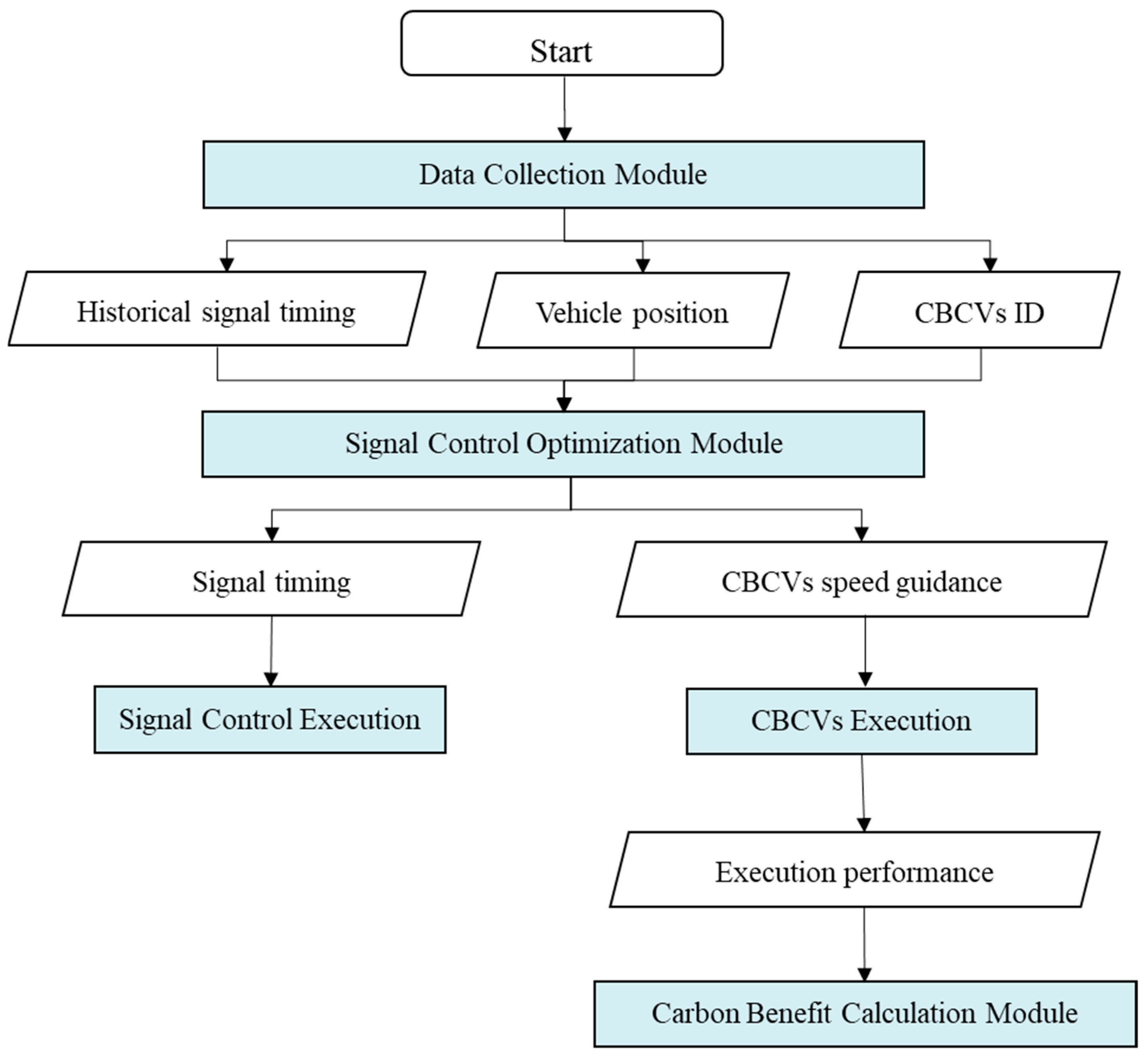
4.2. Control Structure

The control architecture is illustrated in Figure 2. The control system operates within a defined rolling time window, initiating its functions as the designated execution interval commences. It performs data acquisition and identifies CBCVs within the control zone. Following this, the traffic signal control optimization module is activated. This module dispatches command signals to both the traffic controller and CBCVs for execution. Subsequently, the carbon benefit calculation module is activated for evaluation. This control sequence is perpetuated in a rolling time window format. Below are the details of the aforementioned modules.

• Data collection module: This module collects historical signal timing, determines vehicles positions within the control area, and identifies the IDs of CBCVs.
• Signal control optimization module: This module provides the signal timing plan and speed guidance to CBCVs.
• Carbon benefit calculation module: This module evaluates the execution performance of CBCVs based on speed guidance and computes their carbon benefits.

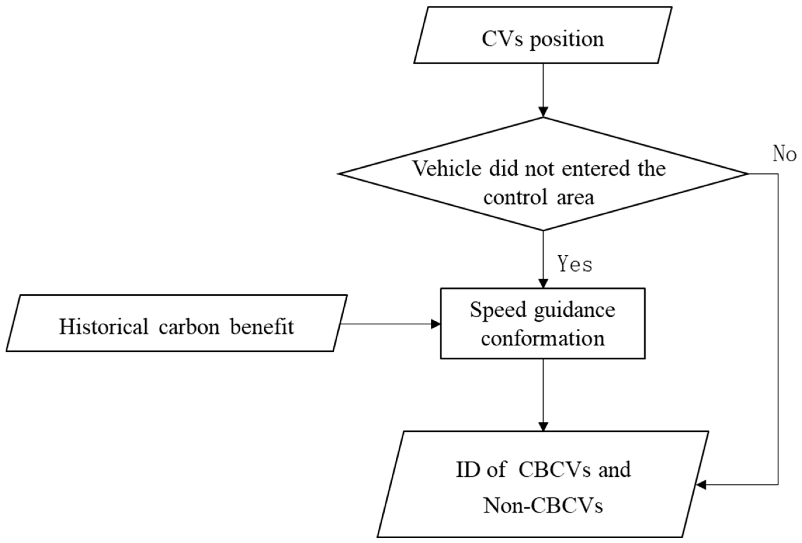
4.3. Data Collection Module

The data collection module collects three main types of information: the historical signal control strategies, the vehicles’ position information, and the IDs of CBCVs.

The historical signal control strategies are the strategies from the previous optimization cycle. These strategies are incorporated into the new optimization round to avoid traffic disruptions caused by abrupt signal changes.

The position information of vehicles is sourced through their vehicular network capabilities, which are utilized to identify which vehicles are within the control zone at the start of the optimization.

The collection of IDs for CBCVs requires identifying which vehicles qualify as CBCVs. This identification is established prior to their entry into the control zone. Outside the control zone, CVs can choose whether to adhere to the speed guidance provided within the zone. If CVs accept the speed guidance, they are designated as CBCVs. To incentivize CVs to accept speed guidance, historical carbon benefits accrued by CBCVs are showcased during the decision-making phase. The process of identifying CBCVs is shown in Figure 3.

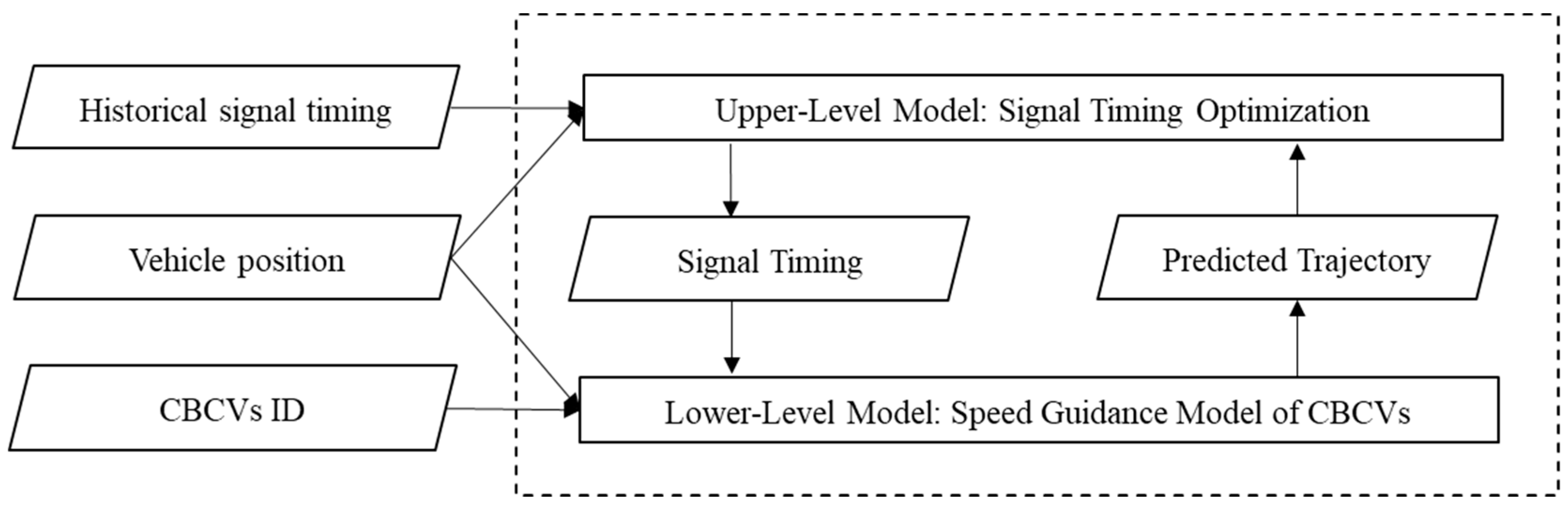
4.4. Signal Control Optimization Module

The goal of this module is to reduce carbon emissions at intersections. In this scenario, the additional emissions originate from speed alterations and stops necessitated by red lights while navigating intersections. The lower the speed of vehicles passing through an intersection, the greater the emissions produced as vehicles accelerate to regain their desired speed.

Building on this analysis, a bi-level optimization model is proposed. At the upper level, signal timing optimization aims to maximize the average speed of vehicles. For computational efficiency, minimizing the vehicles’ delay is employed as a surrogate goal for maximizing average speed, which equivalently contributes to reducing carbon emissions. The lower-level model focuses on optimizing speed recommendations for CBCVs, leveraging the guiding efficacy of CBCVs to minimize the number and duration of vehicle stops. This integrated approach, optimizing both signal timing and vehicle trajectory, significantly reduce emissions, aligning intersection control with environmental sustainability goals. Details are illustrated in Figure 4.

1. 

Upper-level model

The goal of the upper-level model is to reduce delay and indirectly maximize the average speed of vehicles. The objective function is defined as follows:

$$\mathrm{P}1: \underset{\mathit{Y}}{\min }\mathit{T}\mathit{D}$$

(1)

where $\mathit{T}\mathit{D}$ represents the total delay at the intersection. The calculation is as follows:

$$\mathit{T}\mathit{D}=\sum _k\sum _{{\omega }_k\in {\Omega }^k}{D}_{{\omega }_k}$$

(2)

$$\mathit{K}=\left\{\left[{\mathit{k}}_{\mathbf{1}},{\mathit{k}}_{\mathbf{2}},\dots ,{\mathit{k}}_{\mathit{n}}\right]\right\}$$

(3)

where $k$ denotes the phase number and $K$ is the set of all phases within the intersection, which is divided into $n$ phases. Each phase change follows a predetermined sequence. The set ${\Omega }^k$ represents the collection of vehicles within the control area corresponding to phase $k$, and ${\omega }_k$ represents the vehicle number, indicating the ${\omega }_k$-th vehicle in phase $k$. $D_{{\omega }_k}$ denotes the delay of vehicle ${\omega }_k$ during passing through the intersection.

The signal timing plan for the intersection is represented by $\mathit{Y}$.

$$\mathit{Y}=\left\{\left[{\mathit{u}}_{\mathit{k}}^{\mathit{i}},{\mathit{o}}_{\mathit{k}}^{\mathit{i}}\right]\right\},\mathbf{\forall }\mathit{k}\mathbf{\in }\mathit{K};\mathit{i}=\mathbf{1},\dots ,\mathit{N}$$

(4)

where $u_k^i$ represents the start time of the $i$-th green time for phase $k$ within the planning window, and $o_k^i$ represents the end time of the $i$-th green time for phase $k$. $N$ denotes the number of optimization cycles within the model, meaning each optimization provides the control plan for the next $N$ cycles.

a. 

Calculation of Delay

The delay experienced by vehicles is jointly influenced by their trajectory and signal timing, captured by the following formula:

$${\mathit{D}}_{{\mathit{\omega }}_{\mathit{k}}}=\mathit{f}\left({\mathit{x}}^{{\mathit{\omega }}_{\mathit{k}}},\mathit{Y}\right)={\mathit{t}}_{\mathit{c}}^{{\mathit{\omega }}_{\mathit{k}}}+{\mathit{t}}_{\mathit{a}}^{{\mathit{\omega }}_{\mathit{k}}}-{\mathit{t}}_{\mathit{f}\mathit{r}\mathit{e}\mathit{e}}^{{\mathit{\omega }}_{\mathit{k}}},\mathbf{\forall }{\mathit{\omega }}_{\mathit{k}}\mathbf{\in }{\mathit{\Omega }}^{\mathit{k}}$$

(5)

$${\mathit{x}}^{{\omega }_k}={\{x}^{{\omega }_k}\left(t\right)|t=t_0,t_0+∆t,t_0+2∆t\dots ,h_{{\omega }_k}-∆t,h_{{\omega }_k}\}$$

(6)

where ${\mathit{x}}^{{\omega }_k}$ denotes the distance between vehicle ${\omega }_k$ and the stop line, and $h_{{\omega }_k}$ indicates the time when vehicle ${\omega }_k$ crosses the stop line within this window. $t_0$ indicates the start time of the control algorithm. $∆t$ represents the planning time interval. $t_c^{{\omega }_k}$ represents the time at which the vehicle passes the stop line, its calculation taking into account the impact of the signal plan changes on the vehicle’s trajectory. $t_a^{{\omega }_k}$ is the time taken by the vehicle to accelerate from crossing the stop line to its desired speed $v_l$. $t_{free}^{{\omega }_k}$ signifies the time the vehicle spends in free flow to reach the point where it achieves $t_a^{{\omega }_k}$, which is calculated as follows:

$$t_c^{{\omega }_k}=\left\{\begin{array}{c}\mathit{max}\left(u_k^i+{\tau }_f,t_c^{{\omega }_k-1}+\delta \left(d_f\right)\right),o_k^{i-1}<h_{{\omega }_k}<u_k^i\\ \mathit{max}\left(h_{{\omega }_k},t_c^{{\omega }_k-1}+\delta \left(d_f\right)\right),u_k^i<h_{{\omega }_k}<o_k^i\end{array}\right.$$

(7)

$$t_a^{{\omega }_k}={\displaystyle \frac{v_l-v_c}{a_l}}$$

(8)

$$v_c={\displaystyle \frac{x^{{\omega }_k}\left(t_c^{{\omega }_k}\right)-x^{{\omega }_k}\left(t_c^{{\omega }_k}-∆t\right)}{2}}+{\displaystyle \frac{a_l∆t}{2}}$$

(9)

$$t_{free}^{{\omega }_k}={\displaystyle \frac{(v_l-v_c)t_a^{{\omega }_k}}{2v_l}}+{\displaystyle \frac{L}{v_l}}$$

(10)

where $v_c$ is the speed of the vehicle as it crosses the stop line, $v_l$ denotes the speed limit of the road, and $a_l$ represents the maximum acceleration capacity of the vehicle. $\delta \left(d_f\right)$ indicates the time required for the vehicle ${\omega }_k$ to travel a distance $d_f$. $L$ represents the length of the control area.

b. 

Constraints on Signal timing.

In the process of signal optimization, the constraints that must be adhered to include the minimum green time constraint, the maximum green time constraint, the phase sequence constraint, and the clearance time constraint. They are respectively represented as follows:

$$u_k^i+g_{min}\le o_k^i,\forall k\in K;i=1,\dots ,N$$

(11)

$$u_k^i+g_{max}\ge o_k^i,\forall k\in K;i=1,\dots ,N$$

(12)

$$o_k^i\le u_k^{i+1},\forall k\in K;i=1,\dots ,N$$

(13)

$$u_{k_{m+1}}^i\le o_{k_m}^i+t_{clear}$$

(14)

where $t_{clear}$ represents the clearance time required during phase switching. $g_{min}$ denotes the minimum green time duration, $g_{max}$ specifies the maximum green time duration. Equations (11) and (12) are the constraints for the minimum and maximum green time duration of a phase. Equation (13) constrains the start and end times of the signal phase. Equation (14) addresses the constraints on the phase clearance time.

c. 

Constraints on the smoothness of signal timing.

This research adopts a rolling horizon scheme [39]. It is able to continuously collect and update real-time traffic conditions during the optimization process, reducing errors caused by vehicle uncertainties.

In the process of rolling-horizon optimization, the signal timing optimization is repeated in every ${\tau }_{\omega }$. To mitigate the adverse effects of abrupt changes in signal timing updates on traffic, a portion of the timing plan from the previous optimization is retained during each optimization. Specifically, the first optimization occurs at time $t_0$, which is followed by a second optimization at $t_0+{\tau }_{\omega }$. During the second optimization, a safety interval ${\tau }_n$ is introduced to preserve the green phases planned before $t_0+{\tau }_{\omega }+{\tau }_n$. To accommodate this, the model incorporates constraints:

$$u_k^1=\underset{i}{\max }\left\{\left.{u^{\prime }}_k^1\right|{u^{\prime }}_k^1\le t_0+{\tau }_{\omega }+{\tau }_n\right\},\forall kϵK$$

(15)

$$o_k^1=\underset{i}{\max }\left\{\left.{o^{\prime }}_k^1\right|{o^{\prime }}_k^1\le t_0+{\tau }_{\omega }+{\tau }_n\right\},\forall kϵK$$

(16)

where ${u^{\prime }}_k^1$ represents the signal timing solutions from the previous optimization.

2. 

Lower-level model

The goal of the lower-level model is to reduce carbon emissions. The carbon emissions are quantified by the total number of stops and vehicles stop time. The reduction in carbon emissions is achieved by CBCVs’ speed guidance.

The lower-level model is a mixed-integer linear programming (MILP) problem. The objective of the lower-level model is as follows:

$$\mathrm{P}2: \underset{{\mathit{x}}^{{\mathit{\omega }}_{\mathit{k}}^{\mathit{c}}}}{\mathit{min}}J={\sum }_{t_C^k}{p}_f\left({\mathit{x}}^{{\mathit{\omega }}_{\mathit{k}}^{\mathit{c}}}\right)+\alpha p_t\left({\mathit{x}}^{{\mathit{\omega }}_{\mathit{k}}^{\mathit{c}}}\right)$$

(17)

The decision variables are the trajectories of CBCVs, which are denoted as ${\mathit{x}}^{{\mathit{\omega }}_{\mathit{k}}^{\mathit{c}}}$. $p_f\left({\mathit{x}}^{{\mathit{\omega }}_{\mathit{k}}^{\mathit{c}}}\right)$ represents the stop frequency, $p_t\left({\mathit{x}}^{{\mathit{\omega }}_{\mathit{k}}^{\mathit{c}}}\right)$ represents the duration of vehicle stops, and $\alpha$ is the weight of the stop time, with $\alpha \ll 1$. ${\mathit{\Omega }}^{k^c}$ is a regrouping of ${\mathit{\Omega }}^{\mathit{k}}$ based on CBCVs, as follows:

$${\mathit{\Omega }}^{\mathit{k}}=\{\underset{{\Omega }_0^k}{\underbrace{1,2,}}\underset{{\Omega }_1^k}{\underbrace{3^c,4,5,6,}}\underset{{\Omega }_2^k}{\underbrace{7^c,8,9,}}\underset{{\Omega }_3^k}{\underbrace{{10}^c,\dots ,}}\dots \underset{{\Omega }_{{\omega }_k^c}^k}{\underbrace{{{(\omega }_k-m)}^c,\dots ,{\omega }_k-1,{\omega }_k}\}}$$

(18)

$${\mathit{\Omega }}^{k^c}=\{{\Omega }_{{\omega }_k^c}^k,i=0,1,2,\dots {\omega }_k^c\}$$

(19)

where ${\Omega }_0^{k^c}$ denotes the scenario where the lead vehicle of the group is a non-CBCV, occurring only when the first vehicle at the stop line is a non-CBCV.

$p_f\left({\mathit{x}}^{{\omega }_k}\right)$ and $\alpha p_t\left({\mathit{x}}^{{\omega }_k}\right)$ can be calculated as follows:

$$p_f\left({\mathit{x}}^{{\mathit{\omega }}_{\mathit{k}}^{\mathit{c}}}\right)={\sum }_{{\omega }_k}^{{\Omega }_{{\omega }_k^c}^k}{\sum }_{t=t_0}^{h_{{\omega }_k}}{\delta }^{{\omega }_k}\left(t\right)$$

(20)

$$p_f\left({\mathit{x}}^{{\mathit{\omega }}_{\mathit{k}}^{\mathit{c}}}\right)={\sum }_{{\Omega }_{{\omega }_k^c}^k}{\sum }_{t=t_0}{\eta }^{{\omega }_k}\left(t\right)$$

(21)

where $p_f\left({\mathit{x}}^{{\mathit{\omega }}_{\mathit{k}}^{\mathit{c}}}\right)$ represents the total number of stops in the queue with vehicle ${\omega }_k^c$ as the lead vehicle. $p_f\left({\mathit{x}}^{{\mathit{\omega }}_{\mathit{k}}^{\mathit{c}}}\right)$ denotes the total stop time in the queue with vehicle ${\omega }_k^c$ as the lead vehicle. ${\delta }^{{\omega }_k}\left(t\right)$ indicates the number of stops made by vehicle ${\omega }_k$ while passing through the intersection. ${\eta }^{{\omega }_k}\left(t\right)$ represents the stop time of vehicle ${\omega }_k$. These two parameters can be obtained from ${\mathit{x}}^{{\omega }_k}$.

The calculation of $p_f\left({\mathit{x}}^{{\mathit{\omega }}_{\mathit{k}}^{\mathit{c}}}\right)$ and $p_t\left({\mathit{x}}^{{\omega }_k}\right)$ can be derived from the optimized trajectories of CBCVs and the predicted trajectories of non-CBCVs.

a.

Trajectory prediction for non-CBCVs

The trajectories of non-CBCVs can be predicted based on car-following behavior and vehicle location information, as shown below:

$${\mathit{x}}^{{\mathit{\omega }}_{\mathit{k}}}\left(t\right)=f\left({\mathit{x}}^{{\mathit{\omega }}_{\mathit{k}}-\mathbf{1}}\right(t),x^{{\omega }_k}\left(t_0\right),{\tau }_{cf},d_{cf})$$

(22)

${\tau }_{cf}$ and $d_{cf}$ are constants that satisfy the parameters of the Newell car-following model. Equation (22) demonstrates that the trajectory of vehicle ${\mathit{\omega }}_{\mathit{k}}$ is determined by vehicle $({\mathit{\omega }}_{\mathit{k}}-\mathbf{1})$, the initial position, and the parameters of the car-following model.

The prediction method is as follows:

$$x^{{\omega }_k}\left(t\right)=\left\{\begin{array}{c}{x}^{{\omega }_k}\left(t-1\right)+{\mathit{v}}^{{\omega }_k}\left(t-1\right)∆t,u_k^i\le t<o_k^{i+1}\\ 0,r_{{\omega }_k}\left(t\right)=1\end{array}\right.$$

(23)

$${\mathit{v}}^{{\omega }_k}\left(t\right)=\left\{\begin{array}{c}{v}_l,x^{{\omega }_k}\left(t\right)>x^{{\omega }_k-1}\left(t-{\displaystyle \frac{{\tau }_{cf}}{∆t}}\right)+d_{cf}\\ {\mathit{v}}^{{\omega }_k-1},{\mathit{x}}^{{\omega }_k}\left(t\right)=x^{{\omega }_k-1}\left(t-{\displaystyle \frac{{\tau }_{cf}}{∆t}}\right)+d_{cf}\\ 0,r_{{\omega }_k}\left(t\right)=1 and o_k^i\le t<u_k^{i+1}\end{array}\right.$$

(24)

$x^{{\omega }_k}\left(t\right)$ can be divided into two scenarios: when the vehicle is the lead vehicle at the stop line facing a red light on the approach lane and when it is not the lead vehicle, as shown in Equation (23). The term $r_{{\omega }_k}\left(t\right)=1$ indicates whether vehicle ${\omega }_k$ is the leading vehicle at the stop line encountering a red light on the approach. Conversely, $r_{{\omega }_k}\left(t\right)=0$ suggests the opposite scenario. ${\mathit{v}}^{{\omega }_k}\left(t\right)$ denotes the predicted speed of vehicle ${\omega }_k$ at time $t$. This prediction can be categorized into three types: free-flow state, car-following state, and the state where the vehicle is the lead vehicle at the stop line facing a red light on the approach lane, as shown in Equation (24).

The linearization forms of Equations (23) and (24) are as follows:

$$x^{{\omega }_k}\left(t\right)={[x}^{{\omega }_k}\left(t-1\right)+{\mathit{v}}^{{\omega }_k}\left(t-1\right)∆t\left]\right(1-r_{{\omega }_k}\left(t\right))$$

(25)

$${\mathit{v}}^{{\omega }_k}\left(t\right)={[v}_l(1-s_{{\omega }_k}\left(t\right))+{\mathit{v}}^{{\omega }_k-1}{s}_{{\omega }_k}\left(t\right)] (1-r_{{\omega }_k}\left(t\right))$$

(26)

Equation (26) incorporates the logical variable $s_{{\omega }_k}\left(t\right)$. The condition $s_{{\omega }_k}\left(t\right)=0$ holds when ${\mathit{x}}^{{\omega }_k}\left(t\right)=x^{{\omega }_k-1}\left(t-{\displaystyle \frac{{\tau }_{cf}}{∆t}}\right)+d_{cf}$. Otherwise, $s_{{\omega }_k}\left(t\right)=1$.

b.

Target speed optimization for CBCVs

The results of trajectory optimization in the lower-level model will be sent to the vehicle end of CBCVs for execution. However, trajectory-level commands are challenging for CBCVs to execute with precision. Consequently, it is essential to transform these trajectory commands into speed guidance instructions, as shown below:

(a)

Trajectory planning of CBCVs:

The kinematic equation for CBCVs is

$${\mathit{v}}^{{\mathit{\omega }}_{\mathit{k}}}\left(t\right)={\dot{\mathit{x}}}^{{\mathit{\omega }}_{\mathit{k}}}\left(t\right)$$

(27)

$${\mathit{a}}^{{\mathit{\omega }}_{\mathit{k}}}\left(t\right)={\dot{\mathit{v}}}^{{\mathit{\omega }}_{\mathit{k}}}\left(t\right))$$

(28)

where ${\mathit{v}}^{{\mathit{\omega }}_{\mathit{k}}}\left(t\right)$ represents the speed of vehicle ${\mathit{\omega }}_{\mathit{k}}$ at time t, and ${\mathit{a}}^{{\mathit{\omega }}_{\mathit{k}}}\left(t\right)$ represents the acceleration of vehicle ${\mathit{\omega }}_{\mathit{k}}$ at time $t$. The following constraints apply:

Speed limits constrain:

$$0\le {\mathit{v}}^{\mathit{\omega }}\le v_l$$

(29)

Acceleration limits constrain:

$$-a_L^{{\omega }_k}\le {\mathit{a}}^{{\mathit{\omega }}_{\mathit{k}}}\left(t\right)\le a_U^{{\omega }_k}$$

(30)

Vehicle following constraint:

$$x^{{\omega }_k}\left(t\right)\ge x^{{\omega }_k-1}\left(t-{\displaystyle \frac{{\tau }_{cf}}{∆t}}\right)+d_{cf},\forall {\omega }_k\in {\Omega }_k$$

(31)

The trajectory planning for CBCVs is conducted sequentially based on the distance from the vehicle’s initial position to the stop line from the nearest to the farthest vehicle. Once the trajectory of the first vehicle at the stop line is determined, the subsequent vehicle’s identity is assessed: if the following vehicle is a CBCV, its trajectory is planned to ensure compliance with constraints (29) to (31); if the following vehicle is a non-CBCV, its trajectory is predicted according to Equations (25) and (26).

(b)

Speed guidance for CBCVs:

$${\mathit{v}}_{\mathit{s}\mathit{g}}^{{\mathit{\omega }}_{\mathit{k}}^{\mathit{c}}}\left(\mathit{t}\right)=v^{{\omega }_k^c}\left(t_0+i·N_{sg}∆t\right), for i=0,1,2,\dots ,\left[{\displaystyle \frac{h_{{\omega }_k^c}-t_0}{N_{sg}∆t}}\right]$$

(32)

$$v^{{\omega }_k^c}\left(t\right)={\displaystyle \frac{x^{{\omega }_k^c}(t+N_{sg}∆t)-x^{{\omega }_k^c}\left(t\right)}{N_{sg}∆t}}$$

(33)

where $v_{sg}^{{\omega }_k^c}\left(t\right)$ represents the target speed for vehicle ${\omega }_k^c$ at time $t$. The term $N_{sg}∆t$ denotes the transmission interval for speed instructions, during which the vehicle receives a single speed guidance command. $v^{{\omega }_k^c}\left(t\right)$ provides a calculation method for speed instructions with a period of $N_{sg}∆t$.

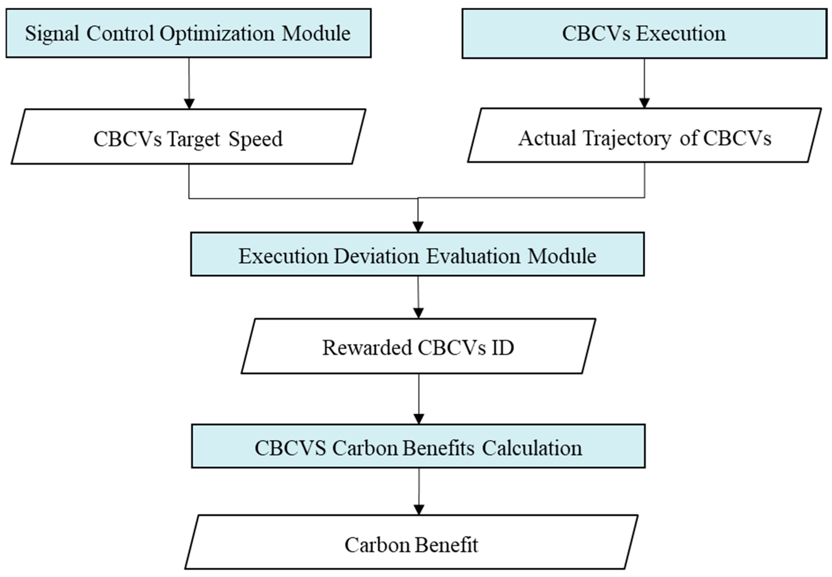
4.5. Carbon Benefit Calculation Module

This section provides a detailed explanation of the carbon emission benefit calculation for CBCVs, as illustrated in Figure 5.

a.

Data Preparation

The data required for the carbon benefit calculation module are divided into two parts. The first part consists of the target speed provided to the CBCVs by the control system, which can be obtained from Equation (32). The second part includes the actual trajectory information of CBCVs as they traverse the controlled intersection area until they pass through. The complete set of these data is obtained after the vehicle has fully passed through the intersection.

b.

Execution Deviation Evaluation Module

Based on the speed guidance from the signal control optimization module’s output for CBCVs and the actual trajectory outputted by the CBCVs execution, the execution deviation evaluation module assesses whether the CBCVs have correctly executed the speed guidance instructions. It determines the IDs of the CBCVs to be rewarded based on the execution. The evaluation is as follows:

$$t_e<TH$$

(34)

$$t_e={\displaystyle \frac{t_0}{h_{{\omega }_k^c}}}·{\sum }_{t=t_0}^{h_{{\omega }_k^c}}{\displaystyle \frac{\left|{\mathit{v}}_{\mathit{s}\mathit{g}}^{{\mathit{\omega }}_{\mathit{k}}^{\mathit{c}}}\left(\mathit{t}\right)-{\mathit{v}}_{\mathit{a}\mathit{t}}^{{\mathit{\omega }}_{\mathit{k}}^{\mathit{c}}}\left(\mathit{t}\right)\right|}{v_{sg}^{{\omega }_k^c}\left(t\right)}}$$

(35)

where $v_{at}^{{\omega }_k^c}\left(t\right)$ represents the actual speed of vehicle ${\omega }_k^c$ at time $t$. $TH$ denotes the threshold for judging whether the vehicle has complied with the speed guidance instructions.

c.

CBCVs Carbon Benefit Calculation

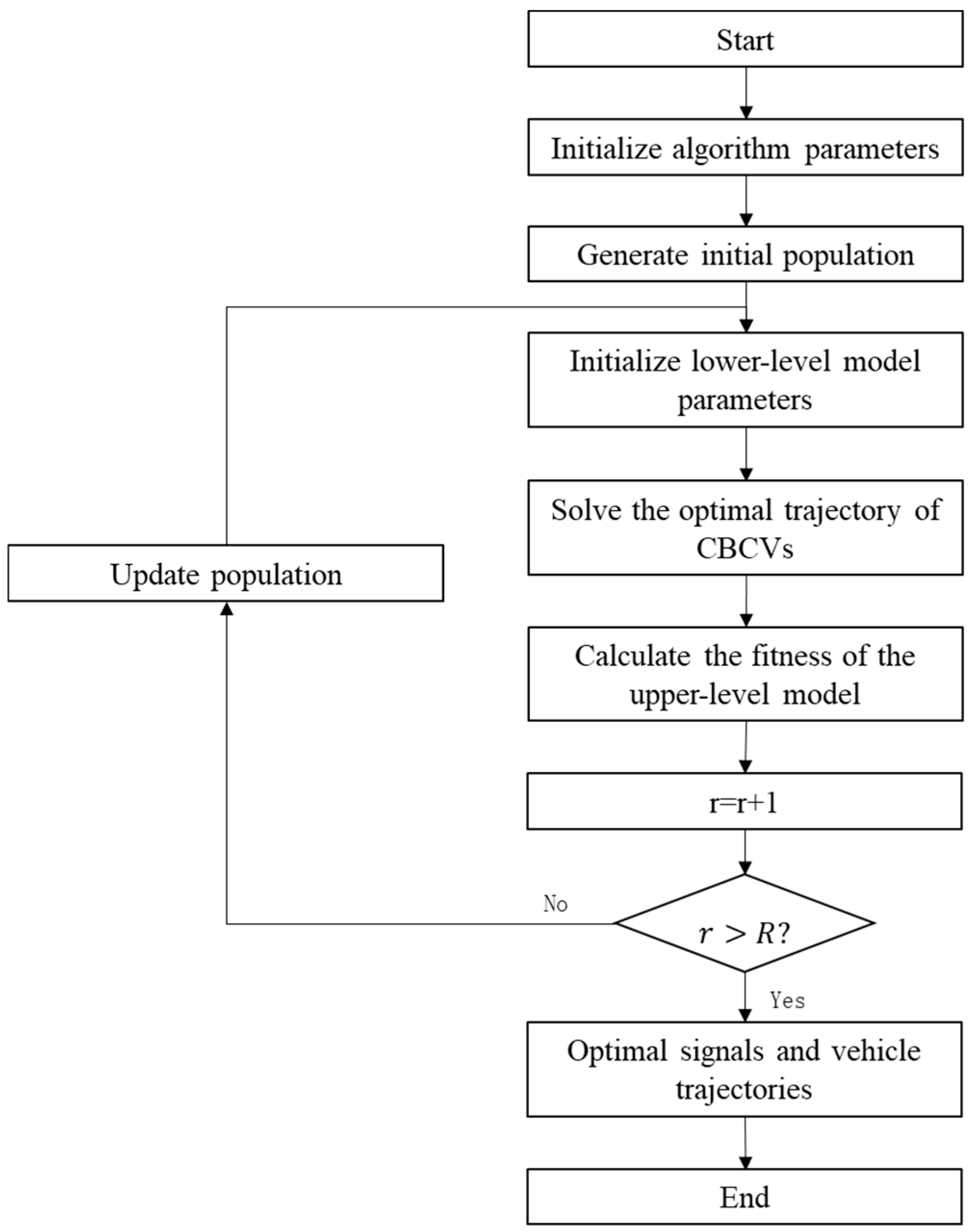
This model will calculate the corresponding carbon reward amounts based on the IDs of CBCVs. The calculation formula is as follows:

$$R\left({\omega }_k^c\right)=CE\left({\omega }_k^c\right)\times CP$$

(36)

$R\left({\omega }_k^c\right)$ represents the carbon reward amount allocated to ${\omega }_k^c$. $CE\left({\omega }_k^c\right)$ denotes the reduction in carbon emissions by vehicle ${\omega }_k^c$ at the intersection. $CP$ represents the incentive amount per unit of carbon emission reduction, which is determined by the pricing of the Chinese carbon trading market.

When quantifying the carbon benefits of CBCVs, there are two components involved. The first part pertains to the reduction in carbon emissions achieved through speed guidance applied to the CBCVs themselves. The second part concerns the emission reduction in non-CBCVs influenced by the guidance effect of the CBCVs. The proposed method determines the guidance effect of CBCVs by grouping vehicles, as shown in Equations (18) and (19). The IDs of non-CBCVs guided by each CBCV can be identified. Their corresponding trajectories can be obtained using Equations (22)–(26). Based on these vehicle trajectories, $CE\left({\omega }_k^c\right)$ can be calculated, as shown below:

$$CE({\omega }_k^c)={CE}_0^{{\omega }_k^c}-{CE}_{opt}^{{\omega }_k^c}$$

(37)

$${CE}_0^{{\omega }_k^c}={\sum }_{{\mathit{\Omega }}^{k^c}}{f}_{ce}\left({\mathit{x}}_{\mathbf{0}}^{{\mathit{\omega }}_{\mathit{k}}}\right)$$

(38)

$${CE}_{opt}^{{\omega }_k^c}={\sum }_{{\mathit{\Omega }}^{k^c}}{f}_{ce}\left({\mathit{x}}^{{\mathit{\omega }}_{\mathit{k}}}\right)$$

(39)

where ${CE}_0^{{\omega }_k^c}$ represents the emissions of all vehicles within the group ${\Omega }^{k^c}$ when vehicle ${\omega }_k^c$ did not implement the speed guidance strategy. ${CE}_{opt}^{{\omega }_k^c}$ denotes the emissions of all vehicles within the group ${\Omega }^{k^c}$ when vehicle ${\omega }_k^c$ had executed the speed guidance strategy. The function $f_{ce}\left(x_0^{{\omega }_k}\right)$ is used to calculate the emissions produced by vehicle ${\omega }_k$ as it passes through an intersection, typically employing a microsimulation model to accurately estimate emissions.

4.6. Solution

In this section, a GA-PSO algorithm is designed to solve the proposed bi-level optimization model, optimizing the signal timing and the optimal trajectories of CBCVs. The methodology proceeds as follows:

Step 1: Initialization. Initialize parameters for the GA-PSO, encompassing population size $N_p$, crossover rate $CR$, mutation rate $MR$, inertia weight $W_i$, cognitive constant $c_1$, social constant $c_2$, and the maximum number of iterations $R$.

Step 2: Generation. Generate $N_p$ initial populations of signal plans, ensuring compliance with signal control constraints Equations (11)–(16).

Step 3: Solution. For each population, solve the standard MILP model P2 to optimize the trajectories ${\mathit{x}}^{{\mathit{\omega }}_{\mathit{k}}^{\mathit{c}}}$ of CBCVs using common solvers and subsequently predict the trajectories of non-CBCVs ${\mathit{x}}^{{\mathit{\omega }}^{\mathit{k}}}$.

Step 4: Fitness Calculation. Evaluate the fitness of each upper-level model configuration using the predicted trajectories and corresponding signal plans.

Step 5: Iteration Check. Assess whether the optimization iteration limit R has been reached. If so, output the optimal result. If not, advance to step 6.

Step 6: Selection and Update. Select individuals with high fitness scores and update the GA-PSO population. This includes selection, crossover, and mutation processes (GA components) as well as updates to velocity and position (PSO components). Subsequently, cycle back to Step 3.

The algorithm flow chart is depicted in Figure 6.

5. Evaluation

This section evaluates the proposed method through microscopic simulation.

5.1. Experiment Design

5.1.1. Testbed

The test scenario for evaluation is presented in Figure 7. It is based on a real intersection located in Yizhuang, Beijing, and is modeled as a 1:1 digital twin in the simulation.

5.1.2. Simulation Platform

To ensure more realistic simulations of real-world traffic scenarios, the simulation platform was developed based on VISSIM and has been enhanced to be applicable to connected traffic environments. This work has undergone peer review and was published in Transportation Research Part C [40]. The simulation environment is a digital twin replication of real-world traffic scenarios. The driving behavior model for connected vehicles is calibrated using naturalistic driving data collected from Yizhuang, Beijing, provided by Amap. Traffic flow changes are calibrated based on roadside detector data from Yizhuang provided by the Beijing Traffic Control Center.

The parameters in the simulation experiment are shown in

Table 2. Simulation settings.

Parameter	Value
Length of the segment under control (m)	300
Simulation duration (s)	1200
The update time interval of signal control (s)	1
Duration of the clearance time (s)	3
Minimum green time interval (s)	15
Maximum green time interval (s)	50
Saturation flow rate (veh/h)	1440
Maximum acceleration (m/s2)	3.5
Minimum acceleration (m/s2)	−4
Time lag in the Newswell model (s)	1.6
Spatial lag in the Newswell model (m)	6
Speed limit of the road (km/h)	60
The average length of vehicles (m)	4.5
The transmission interval for CBCVs speed guidance (s)	3
Execution cycle of the rolling horizon scheme (s)	15
The safety interval in the rolling horizon scheme (s)	5
The gradient of the road segment	0

.

5.1.3. Tested Model

This study conducted tests on two signal control methods: the fixed signal control method and the proposed method. Details are as follows.

Fixed Signal Control Method (Base): In this scenario, the signal control scheme operates on fixed, predetermined signal timings. This method serves as a baseline to illustrate the necessity of optimization.

The Proposed Method: In this scenario, the traffic consists of a mix of CBCVs and non-CBCVs. CBCVs are guided in coordination with the traffic signals. When the proportion of CBCVs is 0, the proposed method is equivalent to an adaptive signal control method.

5.1.4. Sensitivity Analysis

This study conducted a sensitivity analysis on control methods across various traffic demands, different CRs of CBCVs, and unbalanced traffic demand.

The traffic demand level is quantified through the Volume-to-Capacity (V/C) ratio. In the balanced traffic flow scenario, the specific demand levels analyzed are 0.2, 0.5, and 0.8.

The CR of CBCVs are set to 10%, 30%, 50%, and 70%. Sensitivity testing for imbalance traffic demand was conducted with a CBCV CR of 30%. The imbalance in traffic demand reflects the combination of traffic flows in different directions, which can be categorized into the following four types:

(i)

Balanced traffic demand in all directions.

(ii)

Uneven straight-through traffic demand on arteries.

(iii)

Uneven left-turn traffic demand on main arteries.

(iv)

Uneven traffic demand of both straight-through and left-turn traffic on main arteries.

The details are shown in

Table 3. Four unbalanced traffic demand patterns.

Traffic Demand Structure	Traffic Demand (V/C)
	s-n	s-w	e-w	e-s	n-s	n-e	w-e	w-n
I	0.5	0.5	0.5	0.5	0.5	0.5	0.5	0.5
II	0.5	0.5	0.8	0.5	0.5	0.5	0.2	0.5
III	0.5	0.5	0.5	0.8	0.5	0.5	0.5	0.2
IV	0.5	0.5	0.8	0.8	0.5	0.5	0.2	0.2

.

5.1.5. Measurement of Effectiveness

To investigate the effectiveness of the proposed method, three measures of effectiveness (MOE) were adopted: carbon emission, stop frequency, and delay. These measures are used to quantify the performance of the proposed strategies in terms of carbon reduction and transportation efficiency.

Carbon emission and stop frequency are used to assess the degree of ecological improvement. Carbon emissions are calculated using the VSP model. Stop frequency is defined as the average number of stops made by all vehicles and is also used to illustrate the principles behind the control mechanism. The proposed controller achieves carbon reduction by reducing the number of stops.

Delay is used to measure the overall efficiency improvement of intersections. It is defined as the average delay experienced by vehicles passing through the intersection over the entire control period.

5.2. Results

This section presents the simulation results.

5.2.1. Carbon Emission

Figure 8 depicts the carbon emissions and benefits under different demand levels and CRs using the proposed method. The proposed method demonstrates significant benefits across various demand levels, achieving emission reductions ranging from 5.24% to 17.60%. When the penetration rate of CBCVs is zero, the method degrades into an adaptive approach, utilizing only the signal control optimization from the upper-level model yet still achieving benefits ranging from 5.24% to 6.70%. This indicates that despite the method optimizing signal control to minimize delay, it still delivers emission reduction benefits.

Upon introducing CBCVs, the emission reduction benefits increase from 6.62% to 17.60%, demonstrating the advantage of the coordinated optimization framework between signal control and vehicle trajectories within the method. This also validates the effectiveness of the lower-level model, which optimizes based on stopping frequencies and durations, in significantly reducing intersection emissions.

Table 4. Average carbon emissions (g) under different transportation demand structures.

Traffic Demand Structure	Fixed Signal Control Method	Adaptive Signal Control Method	The Proposed Method	Compared to the Fixed Signal Control Method	Compared to the Adaptive Signal Control Method
I	152.3	142.1	130.2	14.51%	8.37%
II	167.1	162.4	147.8	11.55%	8.99%
III	161.2	154.3	140.1	13.09%	9.20%
IV	169.3	161.2	154.2	8.92%	4.34%

displays the average carbon emissions for three control methods under the non-uniform traffic demand. The results indicate that the proposed method exhibits significantly greater advantages under non-uniform traffic conditions. Compared to fixed-timing control, it achieves emission reductions ranging from 8.92% to 14.51%, and compared to adaptive control, it achieves reductions from 4.34% to 9.20%. This is attributed to the study’s ability to optimize the trajectories of CBCVs, influencing other vehicles to adopt more efficient trajectories and maximizing green phase utilization at each intersection. This mitigates the negative impacts of uneven traffic demands effectively.

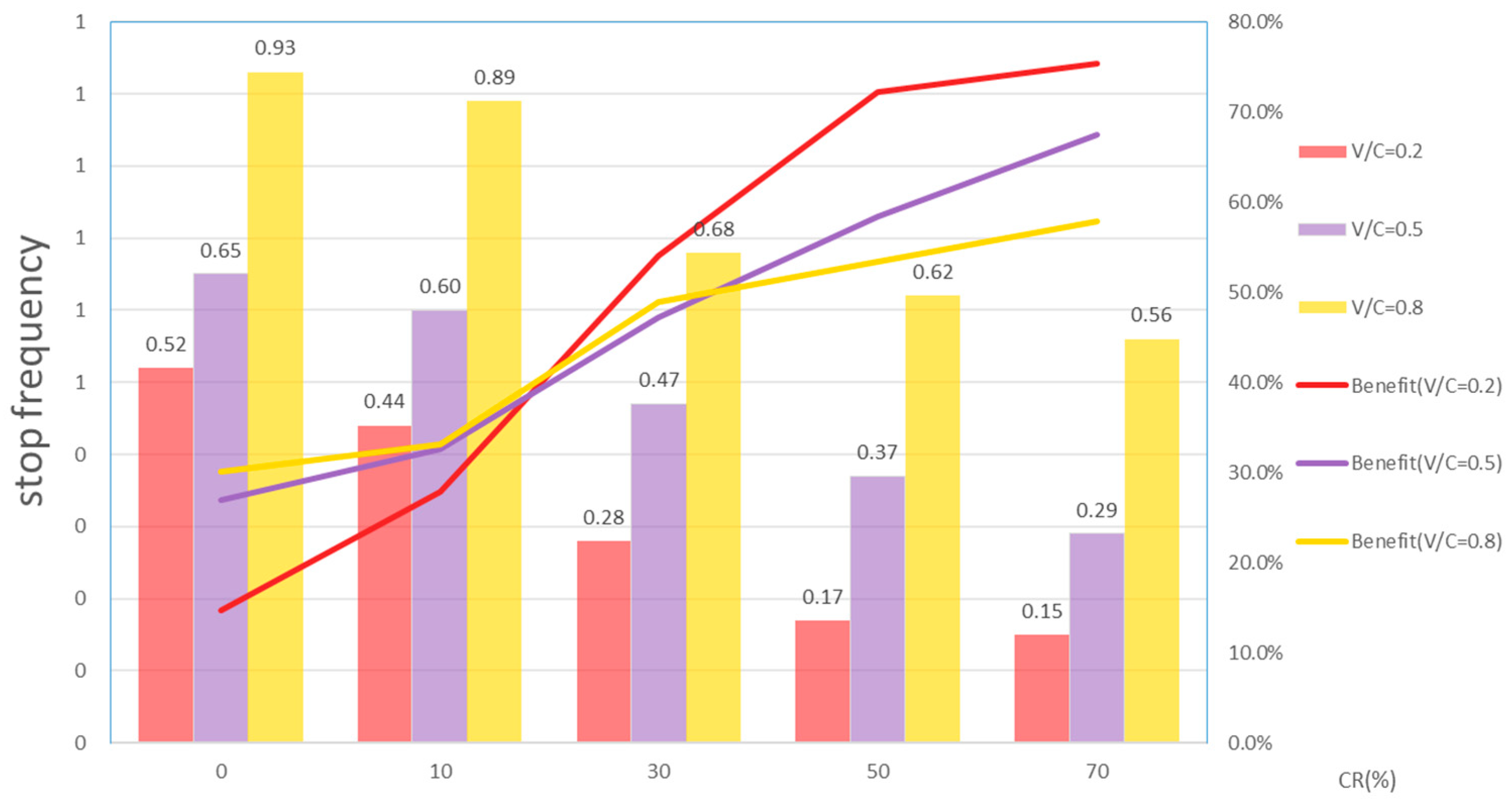
5.2.2. Stop Frequency

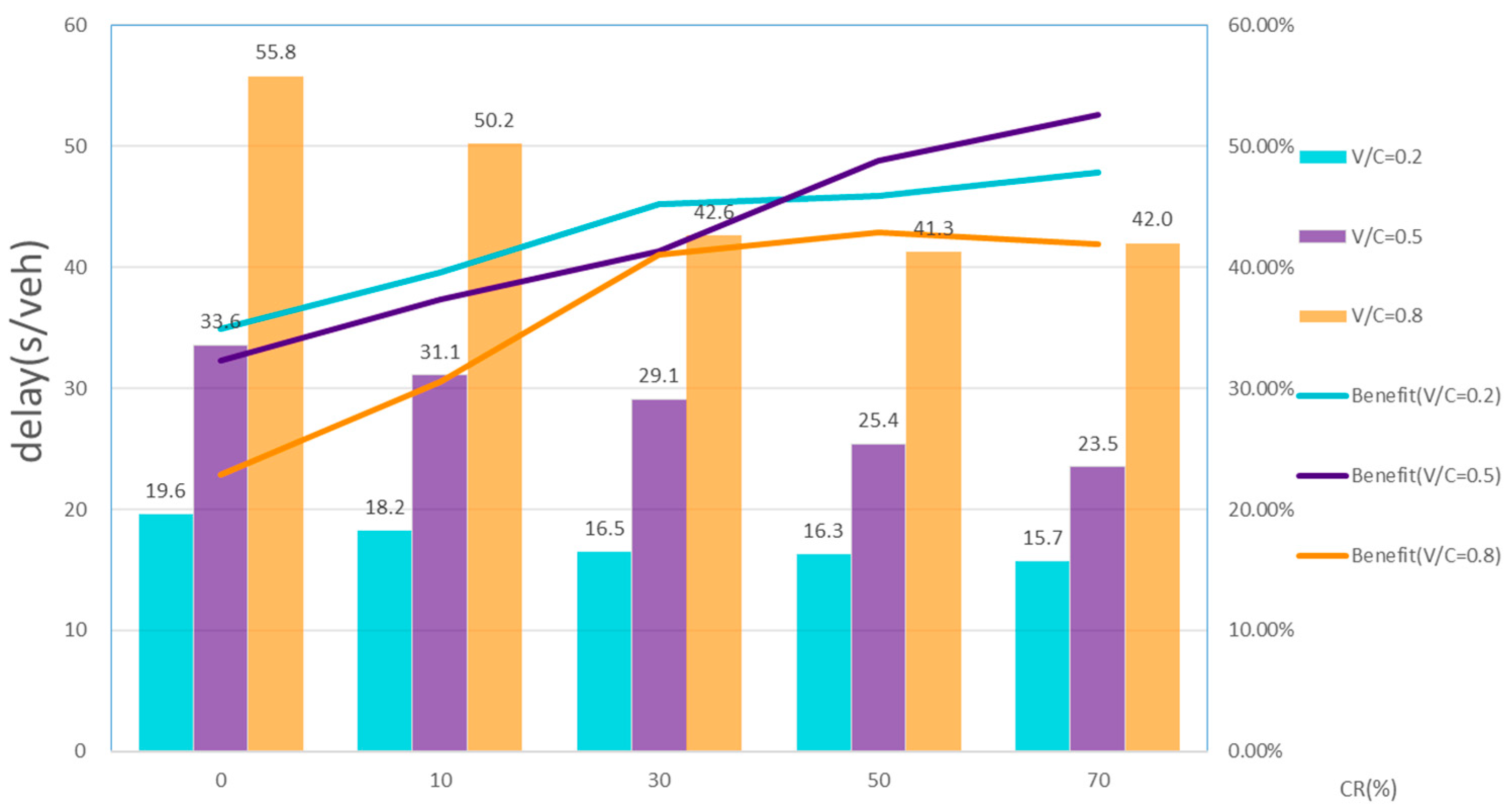
Figure 9 illustrates the stop frequency and benefits under different demand levels and CR using the proposed method. The proposed method demonstrates significant benefits across various demand levels, achieving reductions in average vehicle stops ranging from 14.8% to 75.4%. Optimization benefits of the adaptive control method range from 14.8% to 30.1%, whereas this method achieves benefits ranging from 27.9% to 75.4% with the introduction of CBCVs. Moreover, as the number of CBCVs increases, the benefits of reduced stops become more pronounced. This is because more CBCVs facilitate a smoother passage of vehicles through intersections without stopping. As traffic demand increases, the optimization performance in reducing stops gradually diminishes. This is due to limited optimization opportunities for vehicle trajectory control under higher traffic demands.

Table 5. Stop frequency under different transportation demand structures.

Traffic Demand Structure	Fixed Signal Control Method	Adaptive Signal Control Method	The Proposed Method	Compared to the Fixed Signal Control Method	Compared to the Adaptive Signal Control Method
I	0.89	0.65	0.47	47.19%	27.69%
II	0.97	0.78	0.58	40.21%	25.64%
III	0.93	0.69	0.54	41.94%	21.74%
IV	1.01	0.82	0.59	41.58%	28.05%

displays the stop frequency for three control methods under the unbalanced traffic demand. Compared to fixed-timing control, the proposed method achieves emission reduction benefits ranging from 41.58% to 47.19%. Compared to adaptive control, it achieves benefits ranging from 21.74% to 28.05%. These results indicate that the proposed method exhibits more stable performance under non-uniform traffic flows. This stability arises because the lower-level model targets minimizing stopping frequencies, utilizing coordinated optimization with signals to maximize the method’s potential in reducing stoppages.

5.2.3. Delay

Figure 10 illustrates the delay and benefits under different demand levels and CR using the proposed method. The proposed method demonstrates significant benefits across various demand levels, achieving reductions in delay ranging from 22.82% to 52.62%. Optimization benefits of the adaptive control method range from 22.82% to 34.88%, whereas with the inclusion of CBCVs, reductions in delay range from 30.57% to 52.62%. This proves that the proposed method can improve the ceiling of travel efficiency at intersections.

At V/C ratios of 0.2 and 0.5, the increase in CBCVs yields positive but not significant benefits. At a V/C ratio of 0.8, a 30% penetration of CBCVs achieves maximum optimization benefits but thereafter shows a declining trend. This is because under high traffic demand, the optimization space for CBCVs is limited. In this method, signal control optimization significantly influences delay reduction, especially at high V/C ratios, whereas vehicle control focuses more on emission reduction, potentially causing conflicts and compromising delay reduction benefits.

Table 6. Average delay (s) under different transportation demand structures.

Traffic Demand Structure	Fixed Signal Control Method (s)	Adaptive Signal Control Method (s)	The Proposed Method (s)	Compared to the Fixed Signal Control Method	Compared to the Adaptive Signal Control Method
I	49.6	33.6	29.1	41.33%	13.39%
II	52.1	33.9	29.5	43.38%	12.98%
III	51.1	34.1	30.1	41.10%	11.73%
IV	52.9	35.1	30.2	42.91%	13.96%

presents the delay results for three control methods under the unbalanced traffic demand. The results indicate significant optimization of the proposed method under non-uniform traffic flows. Compared to fixed-timing control, the proposed method achieves emission reduction benefits ranging from 41.10% to 43.38%. This is due to the rolling optimization framework adopted in signal optimization, which effectively captures and predicts vehicle arrivals within each optimization cycle to implement the most optimal control strategy. Compared to adaptive control, the inclusion of CBCVs provides an additional optimization space of 11.73% to 13.96%. This is because vehicle arrivals are optimized by the trajectory control in the lower-level model, further enhancing the ceiling of intersection control efficiency.

5.2.4. Carbon Benefits

Figure 11 illustrates the carbon benefits of CBCVs. The carbon reduction rewards are benchmarked against the current price in China’s carbon trading market, which is valued at RMB 90 per ton of carbon dioxide reduced. At this pricing, the average reward per CBCV ranges between RMB 0.0015 and 0.0165, exhibiting a certain regularity.

As the CR of CBCVs increases, the average carbon revenue per CBCV declines. This is because when the proportion of CBCVs in the traffic flow is relatively low, the actions of each CBCV can influence more non-CBCVs, thus improving the carbon benefits from the perspective of individual vehicles. Conversely, as the proportion of CBCVs in the traffic flow increases, fewer non-CBCVs can be influenced. For instance, at a 70% CR, only 30% of the vehicles are non-CBCVs, meaning that on average, only one out of every two CBCVs will influence a non-CBCV. In high CR environments, the guidance role of CBCVs is shared among many vehicles, reducing the number of non-CBCVs that each CBCV can influence, lowering the carbon reward per CBCV. Although the collective carbon reduction capacity of CBCVs remains, the contribution of each CBCV is diluted, leading to reduced individual carbon rewards.

With increasing traffic demand, the average carbon revenue per CBCV shows an upward trend, indicating that CBCVs can achieve higher carbon reduction rewards under busy traffic conditions. When the v/c is 0.2, the average rewards per vehicle range from RMB 0.0015 to 0.0021. When the v/c ratio is 0.5, the average rewards per vehicle range from RMB 0.0047 to 0.0057. When the v/c ratio is 0.8, the average rewards per vehicle range from RMB 0.0085 to 0.0165. This is because increased traffic demand leads to denser traffic flow, allowing CBCVs to influence more non-CBCVs through their speed strategies. Additionally, the increase in traffic volume generally results in higher per-vehicle carbon emissions, providing more room for emission reduction through the guiding effectiveness of each CBCV.

6. Discussion

6.1. Summary and Analysis of the Results

The comparison between the proposed method and the baseline confirms the significant advantages of the proposed approach. Under varying traffic demands, the benefits of the proposed method include a reduction in carbon emissions by 5.24% to 17.60%, a decrease in stop frequency by 14.8% to 75.4%, and a reduction in delay by 22.82% to 52.62%. Moreover, under conditions of unbalanced traffic demand, the proposed method achieves a reduction in carbon emissions by 8.92% to 14.51%, a decrease in stop frequency by 41.58% to 47.19%, and a reduction in delay by 41.10% to 43.38%.

A notable highlight of the proposed method is the integration of CIM with traffic control. Specifically, the approach leverages carbon pricing from the carbon trading market to calculate the emission reductions achieved by CBCVs that follow intersection speed guidance instructions and subsequently provide financial rewards. This study represents the first exploration of such a method. Figure 12 provides a comprehensive illustration of the carbon reduction costs associated with the proposed method at intersections: the rewards provided to CBCVs for each ton of carbon emission reduction at the intersection range from RMB 7.5 to 31.5. This cost is lower than the carbon trading market price of 90 RMB/t of carbon dioxide, indicating that the trading price in the carbon market can fully cover the financial rewards given to CBCVs. The difference arises because the emission reductions at the intersection are due to both signal control and vehicle speed guidance. The emission reduction benefits from signal optimization are not used for reward distribution. In practical applications, this portion of funds could be allocated to cover the costs of signal optimization. Another viable approach could be to increase the financial rewards given to CBCVs, enhancing economic incentives for drivers to adopt eco-driving habits.

6.2. Advantages and Limitations

The primary advantage of the proposed method lies in its ability to achieve emission reductions through the coordination of signal control and vehicle guidance when compared to the existing literature.

Reference [12] proposed an eco-oriented signal control method that reduces ecological costs by 13.57% but requires a 4.84% increase in vehicle delay. The method proposed in this paper, when applied in scenarios with zero CBCVs, functions as a purely signal-based adaptive control approach that can reduce emissions by 5.24% to 6.70% without compromising vehicle delay benefits. Compared to reference [11], the proposed method ensures a balanced multi-objective optimization at intersections by considering delay reduction as part of the optimization goals.

Reference [29] developed a multi-vehicle cooperative eco-driving system for signalized intersections under partial CAV environments, achieving a 10.95% reduction in carbon emissions in scenarios with fixed-timed signals. The proposed method, by utilizing the coordinated optimization of signals and vehicles, achieved a maximum emission reduction of 17.60% in experiments, outperforming the results of reference [29], thus demonstrating the necessity of coordination.

Despite the significant advantages of the proposed method in achieving emission reductions at intersections, there are certain limitations. It was observed that under highly congested traffic conditions (v/c > 0.8), the proposed controller could not significantly reduce the number of stops, leading to the failure of the emission reduction function. This is because under extremely congested conditions, the low-speed movement of CBCVs on road segments can cause traffic collapse—a phenomenon described as “phantom jams” on urban roads in reference [4]. Vehicles obstructed by such jams will stop on the road segment and disrupt the flow of subsequent traffic. Furthermore, the proposed control method tends to allow vehicles within the controlled area to stop at most once while passing through the intersection, leading to longer cycle lengths. This may result in optimal phase cycles exceeding the maximum cycle limit, making it difficult to handle highly congested intersections. In fact, congested intersections should not sacrifice delay and maximum throughput in pursuit of overall emission reduction, as this may lead to overflow at the intersection.

6.3. Prospects for Application

The issue of carbon emission reduction is a global concern. The proposed method addresses the need for vehicles at intersections to follow speed guidance to achieve carbon reduction goals by proposing a framework that integrates CIM, carbon trading markets, and intelligent transportation systems. On the one hand, the method achieves eco-driving guidance at intersections by providing financial incentives to drivers. On the other hand, it optimizes both signal control and vehicle guidance in a coordinated manner, raising the upper limit of emission reduction efficiency at intersections. The proposed method’s implementation requires only a connected environment, which significantly enhances its potential for widespread application.

The application of the proposed method involves several key areas. First, it is essential to establish an accurate carbon emission accounting mechanism that can be applied to various traffic control demands. This effort requires government involvement in setting relevant policies. Second, the development of a system or application to transmit intersection speed guidance instructions to vehicles is necessary. This system should be widely accessible with navigation apps on smartphones being a potential solution. Third, the influence of the financial reward amount on driver motivation warrants further exploration, potentially involving research in economics and behavioral science.

7. Conclusions

This study introduces a novel carbon benefits-based signal control method within a connected vehicle (CV) environment. The proposed method uniquely integrates a carbon incentive mechanism with signal control to enhance vehicle compliance with speed guidance, aiming to reduce carbon emissions at signalized intersections. By optimizing signal timing and vehicle speed guidance in a coordinated manner, the method effectively minimizes vehicle speed fluctuations, significantly contributing to emission reduction.

The performance of the proposed method was evaluated using a microscopic simulation platform, demonstrating its effectiveness across various traffic demand scenarios and different penetration rates of connected and automated vehicles (CBCVs). The results indicate that the proposed method achieves substantial reductions in carbon emissions, stop frequencies, and vehicle delays compared to both fixed-timing and adaptive signal control methods. Specifically, carbon emissions were reduced by 5.24% to 17.60%, stop frequencies decreased by 14.8% to 75.4%, and delays were reduced by 22.82% to 52.62%. Under non-uniform traffic conditions, the emission reductions ranged from 8.92% to 14.51% compared to fixed-timing control and from 4.34% to 9.20% compared to adaptive control (when CR is zero in the proposed method).

Furthermore, the proposed method provides a comprehensive framework for calculating carbon emission reductions and corresponding economic incentives for vehicles adhering to speed guidance. According to the carbon incentive framework, the average reward per CBCV ranges between RMB 0.0015 and 0.0165. Correspondingly, the rewards provided to CBCVs for each ton of carbon emission reduction at the intersection range from RMB 7.5 to 31.5. While the carbon rewards based solely on emission reductions may be modest for individual vehicles, they offer a new perspective. Traffic managers can provide additional rewards to encourage vehicle participation in carbon-incentive traffic control methods. These additional rewards can be proportionally distributed based on actual emission reductions, potentially achieving better incentive effects.

Future research could focus on both theoretical and practical advancements in this study. On the theoretical side, it is important to examine how the proposed incentive amounts influence drivers’ motivation to participate. Additionally, integrating CIM with broader traffic management systems, such as multi-intersection signal control or route-based traffic control, could further enhance its environmental and operational benefits. On the practical side, the priority should be to establish an accurate carbon emission pricing mechanism that aligns with both government policies and consumer demands.

References

1. Agency (IEA). CO2 Emissions in 2022; International Energy Agency: Paris, France, 2023. [Google Scholar]
2. Lents, J.; Nikkila, N. IVE Model User Manual (Version 1.1.1); International Sustainable Systems Research Center (ISSRC), EUA: La Habra, CA, USA, 2004. [Google Scholar]
3. Liu, H.; He, K.; Barth, M. Traffic and emission simulation in China based on statistical methodology. Atmos. Environ. 2011, 45, 1154–1161. [Google Scholar] [CrossRef]
4. Kang, Z.; An, L.; Lai, J.; Yang, X.; Sun, W. Eco-Speed Harmonization with Partially Connected and Automated Traffic at an Isolated Intersection. J. Adv. Transp. 2023, 2023, 9948462. [Google Scholar] [CrossRef]
5. Zhong, S.; Zhao, Y.; Ge, L.; Shan, Z.; Ma, F. Vehicle State and Bias Estimation Based on Unscented Kalman Filter with Vehicle Hybrid Kinematics and Dynamics Models. Automot. Innov. 2023, 6, 571–585. [Google Scholar] [CrossRef]
6. Feng, Y.; Head, K.L.; Khoshmagham, S.; Zamanipour, M. A real-time adaptive signal control in a connected vehicle environment. Transp. Res. Part C Emerg. Technol. 2015, 55, 460–473. [Google Scholar] [CrossRef]
7. Chen, S.; Sun, D.J. An improved adaptive signal control method for isolated signalized intersection based on dynamic programming. IEEE Intell. Transp. Syst. Mag. 2016, 8, 4–14. [Google Scholar] [CrossRef]
8. Ren, Y.; Wang, Y.; Yu, G.; Liu, H.; Xiao, L. An adaptive signal control scheme to prevent intersection traffic blockage. IEEE Trans. Intell. Transp. Syst. 2016, 18, 1519–1528. [Google Scholar] [CrossRef]
9. Yao, Z.; Jiang, Y.; Zhao, B.; Luo, X.; Peng, B. A dynamic optimization method for adaptive signal control in a connected vehicle environment. J. Intell. Transp. Syst. 2020, 24, 184–200. [Google Scholar] [CrossRef]
10. Zheng, L.; Li, X. Simulation-based optimization method for arterial signal control considering traffic safety and efficiency under uncertainties. Comput.-Aided Civ. Infrastruct. Eng. 2023, 38, 640–659. [Google Scholar] [CrossRef]
11. Koch, L.; Brinkmann, T.; Wegener, M.; Badalian, K.; Andert, J. Adaptive Traffic Light Control with Deep Reinforcement Learning: An Evaluation of Traffic Flow and Energy Consumption. IEEE Trans. Intell. Transp. Syst. 2023, 24, 15066–15076. [Google Scholar] [CrossRef]
12. Lin, Y.; Guan, H.; Lu, K.; Ma, Y.; Zhao, S. Eco-oriented signal control of intersections with vehicle type considerations using integrated estimation of driving behavior. J. Clean. Prod. 2022, 375, 133986. [Google Scholar] [CrossRef]
13. Tang, T.-Q.; Zhang, J.; Liu, K. A speed guidance model accounting for the driver’s bounded rationality at a signalized intersection. Phys. A Stat. Mech. Its Appl. 2017, 473, 45–52. [Google Scholar] [CrossRef]
14. Almannaa, M.H.; Chen, H.; Rakha, H.A.; Loulizi, A.; El-Shawarby, I. Field implementation and testing of an automated eco-cooperative adaptive cruise control system in the vicinity of signalized intersections. Transp. Res. Part D Transp. Environ. 2019, 67, 244–262. [Google Scholar] [CrossRef]
15. Li, D.; Zhang, K.; Dong, H.; Wang, Q.; Li, Z.; Song, Z. Physics-augmented data-enabled predictive control for eco-driving of mixed traffic considering diverse human behaviors. IEEE Trans. Control. Syst. Technol. 2024, 32, 1479–1486. [Google Scholar] [CrossRef]
16. Naeem, H.M.Y.; Butt, Y.A.; Ahmed, Q.; Bhatti, A.I. Optimal-Control-Based Eco-Driving Solution for Connected Battery Electric Vehicle on a Signalized Route. Automot. Innov. 2023, 6, 586–596. [Google Scholar] [CrossRef]
17. Chen, P.; Yan, C.; Sun, J.; Wang, Y.; Chen, S.; Li, K. Dynamic eco-driving speed guidance at signalized intersections: Multi vehicle driving simulator based experimental study. J. Adv. Transp. 2018, 2018, 6031764. [Google Scholar] [CrossRef]
18. Yu, S.; Fu, R.; Guo, Y.; Xin, Q.; Shi, Z. Consensus and optimal speed advisory model for mixed traffic at an isolated signalized intersection. Phys. A Stat. Mech. Its Appl. 2019, 531, 121789. [Google Scholar] [CrossRef]
19. Zhang, Z.; Zou, Y.; Zhang, X.; Zhang, T. Green light optimal speed advisory system designed for electric vehicles considering queuing effect and driver’s speed tracking error. IEEE Access 2020, 8, 208796–208808. [Google Scholar] [CrossRef]
20. Rabinowitz, A.I.; Ang, C.C.; Mahmoud, Y.H.; Araghi, F.M.; Meyer, R.T.; Kolmanovsky, I.; Asher, Z.D.; Bradley, T.H. Real-time implementation comparison of urban eco-driving controls. IEEE Trans. Control. Syst. Technol. 2023, 32, 143–157. [Google Scholar] [CrossRef]
21. Tajalli, M.; Hajbabaie, A. Traffic signal timing and trajectory optimization in a mixed autonomy traffic stream. IEEE Trans. Intell. Transp. Syst. 2021, 23, 6525–6538. [Google Scholar] [CrossRef]
22. Liu, H.; Lu, X.-Y.; Shladover, S.E. Traffic signal control by leveraging cooperative adaptive cruise control (CACC) vehicle platooning capabilities. Transp. Res. Part C Emerg. Technol. 2019, 104, 390–407. [Google Scholar] [CrossRef]
23. Yao, Z.; Zhao, B.; Yuan, T.; Jiang, H.; Jiang, Y. Reducing gasoline consumption in mixed connected automated vehicles environment: A joint optimization framework for traffic signals and vehicle trajectory. J. Clean. Prod. 2020, 265, 121836. [Google Scholar] [CrossRef]
24. Pourmehrab, M.; Elefteriadou, L.; Ranka, S.; Martin-Gasulla, M. Optimizing signalized intersections performance under conventional and automated vehicles traffic. IEEE Trans. Intell. Transp. Syst. 2019, 21, 2864–2873. [Google Scholar] [CrossRef]
25. Niroumand, R.; Tajalli, M.; Hajibabai, L.; Hajbabaie, A. Joint optimization of vehicle-group trajectory and signal timing: Introducing the white phase for mixed-autonomy traffic stream. Transp. Res. Part C Emerg. Technol. 2020, 116, 102659. [Google Scholar] [CrossRef]
26. Guo, Y.; Ma, J. DRL-TP3: A learning and control framework for signalized intersections with mixed connected automated traffic. Transp. Res. Part C Emerg. Technol. 2021, 132, 103416. [Google Scholar] [CrossRef]
27. Hu, J.; Li, S.; Wang, H.; Wang, Z.; Barth, M.J. Eco-approach at an isolated actuated signalized intersection: Aware of the passing time window. J. Clean. Prod. 2024, 435, 140493. [Google Scholar] [CrossRef]
28. Hu, Y.; Yang, P.; Zhao, M.; Li, D.; Zhang, L.; Hu, S.; Hua, W.; Ji, W.; Wang, Y.; Guo, J. A generic approach to eco-driving of connected automated vehicles in mixed urban traffic and heterogeneous power conditions. IEEE Trans. Intell. Transp. Syst. 2023, 24, 11963–11980. [Google Scholar] [CrossRef]
29. Wang, Z.; Wu, G.; Hao, P.; Barth, M.J. Cluster-wise cooperative eco-approach and departure application for connected and automated vehicles along signalized arterials. IEEE Trans. Intell. Veh. 2018, 3, 404–413. [Google Scholar] [CrossRef]
30. Hill, C.J.; Garrett, J.K. AASHTO Connected Vehicle Infrastructure Deployment Analysis; Joint Program Office for Intelligent Transportation Systems: Washington, DC, USA, 2011. [Google Scholar]
31. Shukla, P.R.; Skea, J.; Slade, R.; Al Khourdajie, A.; Van Diemen, R.; McCollum, D.; Pathak, M.; Some, S.; Vyas, P.; Fradera, R. Climate change 2022: Mitigation of climate change. Contrib. Work. Group III Sixth Assess. Rep. Intergov. Panel Clim. Change 2022, 10, 9781009157926. [Google Scholar]
32. Shahbaz, M.; Li, J.; Dong, X.; Dong, K. How financial inclusion affects the collaborative reduction of pollutant and carbon emissions: The case of China. Energy Econ. 2022, 107, 105847. [Google Scholar] [CrossRef]
33. Chen, Z.; Du, H.; Li, J.; Southworth, F.; Ma, S. Achieving low-carbon urban passenger transport in China: Insights from the heterogeneous rebound effect. Energy Econ. 2019, 81, 1029–1041. [Google Scholar] [CrossRef]
34. Ghate, A.T.; Qamar, S. Carbon footprint of urban public transport systems in Indian cities. Case Stud. Transp. Policy 2020, 8, 245–251. [Google Scholar] [CrossRef]
35. Li, X.; Tan, X.; Wu, R.; Xu, H.; Zhong, Z. Paths for Carbon Peak and Carbon Neutrality in Transport Sector in China. Strateg. Study CAE 2021, 23, 15–21. [Google Scholar] [CrossRef]
36. Ghosh, A. Possibilities and challenges for the inclusion of the electric vehicle (EV) to reduce the carbon footprint in the transport sector: A review. Energies 2020, 13, 2602. [Google Scholar] [CrossRef]
37. Li, R.; Fang, D.; Xu, J. Does China’s carbon inclusion policy promote household carbon emissions reduction? Theoretical mechanisms and empirical evidence. Energy Econ. 2024, 132, 107462. [Google Scholar] [CrossRef]
38. Yu, L.; Liu, Y.; Cheng, Y.; Zhou, Y. Carbon Inclusion for Green Travel and Practices in Beijing. Urban Transp. China 2024, 22, 67–73. [Google Scholar]
39. Ma, C.; Yu, C.; Zhang, C.; Yang, X. Signal timing at an isolated intersection under mixed traffic environment with self-organizing connected and automated vehicles. Comput.-Aided Civ. Infrastruct. Eng. 2023, 38, 1955–1972. [Google Scholar] [CrossRef]
40. Lai, J.; Hu, J.; Cui, L.; Chen, Z.; Yang, X. A generic simulation platform for cooperative adaptive cruise control under partially connected and automated environment. Transp. Res. Part C Emerg. Technol. 2020, 121, 102874. [Google Scholar] [CrossRef]
Figure 1. Illustration of the scenario.
Applsci 14 07638 g001
Figure 2. Control structure.
Applsci 14 07638 g002
Figure 3. The process of identifying CBCVs and non-CBCVs.
Applsci 14 07638 g003
Figure 4. The signal control optimization module.
Applsci 14 07638 g004
Figure 5. Carbon benefit calculation module.
Applsci 14 07638 g005
Figure 6. Algorithm flow chart.
Applsci 14 07638 g006
Figure 7. Tested scenario. (a) Bird view of the intersection. (b) Intersection built in simulation.
Applsci 14 07638 g007
Figure 8. Average carbon emissions (g) and benefits (%) compared with the baseline.
Applsci 14 07638 g008
Figure 9. Stop frequency and benefits (%) compared with the baseline.
Applsci 14 07638 g009
Figure 10. Average delay (s) and benefits (%) compared with the baseline.
Applsci 14 07638 g010
Figure 11. Carbon benefits of CBCVs under different v/c. (a) v/c = 0.2; (b) v/c = 0.5; (c) v/c = 0.8.
Applsci 14 07638 g011
Figure 12. Cost of carbon reduction at intersections.
Applsci 14 07638 g012