Abstract
One technique that is widely used in various fields, including nonlinear target tracking, is the extended Kalman filter (EKF). The well-known minimum mean square error (MMSE) criterion, which performs magnificently under the assumption of Gaussian noise, is the optimization criterion that is frequently employed in EKF. Further, if the noises are loud (or heavy-tailed), its performance can drastically suffer. To overcome the problem, this paper suggests a new technique for maximum correntropy EKF with nonlinear regression (MCCEKF-NR) by using the maximum correntropy criterion (MCC) instead of the MMSE criterion to calculate the effectiveness and vitality. The preliminary estimates of the state and covariance matrix in MCKF are provided via the state mean vector and covariance matrix propagation equations, just like in the conventional Kalman filter. In addition, a newly designed fixed-point technique is used to update the posterior estimates of each filter in a regression model. To show the practicality of the proposed strategy, we propose an effective implementation for positioning enhancement in GPS navigation and radar measurement systems.
1. Introduction
Due to the extensive variety of significant uses in technology, including target tracking, navigation, posture determination, automation, and telecommunications, the filtering approaches for estimating states in dynamical models with state space have gained a lot of interest in the past few decades [1,2,3,4]. It is well known that the best estimations for a linear Gaussian system are Kalman filters (KFs). On the other hand, the optimum or analytical solutions of the posterior probability density functions (PDFs) are typically not accessible for a nonlinear Gaussian system. Thus, the extended Kalman filter (EKF) [5] is a common nonlinear Kalman-type filter that uses first-order linearization to give an estimate of the nonlinear equation before completing the operation of filtering using the traditional KF approach. Additionally, the unscented Kalman filter (UKF) [6], the cubature Kalman filter (CKF) [7], and the Gaussian–Hermite Kalman filter [8] are a few examples of nonlinear filters with less optimality that have been paid more attention for several years.
Furthermore, the above-mentioned nonlinear filters result inappropriately when they are implemented in a situation coupled with non-Gaussian noise. There is the possibility that estimation accuracy will be affected, which may be due to third-party interference or inaccurate sensors from the state and the measurement outliers [9]. Later, several kinds of robust nonlinear filters were designed by integrating the design principles of the Gaussian approximation KF with the robustness cost function developed from Huber’s M-estimation [10]. Another commonly used approach for describing non-Gaussian noise is by employing Student’s t distribution along with the polynomial decay property [11]. This method takes into account the heavy-tailed nature of non-Gaussian noise. On the basis of these ideas, several researchers have introduced the variational Bayes nonlinear filter (VBNF) and the Student’s t-based robust nonlinear filter (RSTNF) [12]. The PDF with the posterior state vector is still a Student’s t PDF having the fixed-point iterations in the RSTNF, where the non-Gaussian processing and the measured noises are considered as Student’s t PDFs having the same degree of freedom (DoF) criteria [13]. VBNFs consider the process noise which has a Gaussian distribution that incurs the danger of worse estimation performance when it is used with non-Gaussian process noise [14].
To overcome the problems associated with the non-Gaussian noises, correntropy has been used for the process [15]. For the linear non-Gaussian frameworks, the maximum correntropy-based Kalman filters were initially suggested in [16]. Beside this, researchers have also focused on the optimization criteria in information theoretic learning (ITL) [17] in recent years. By incorporating the ITL values, the estimation can be calculated straight from the source. Correntropy is one of the information-theoretic quantities; it has been used recently as a reliable cost to deliver notable performance improvements in various sectors for different applications [17,18]. It is capable of capturing higher-order statistics of losses. The novel maximum correntropy extended Kalman filter (MCEKF) has been provided as a solution to this issue [19]. More precisely, the maximal correntropy criterion (MCC) in ITL refers to the optimization criterion for correntropy [20,21]. Many investigations have been carried out on filters against heavy-tailed non-Gaussian noises with robustness adaptivity for GPS navigations with effective performance [22,23]. Further, EKF, multiple-model filters, and modelling noise followed by a Gaussian distribution are used to increase resilience against the outliers, but computational complexity and effort will always be a limiting factor.
On the other hand, iterative techniques are frequently utilized to reach an MCC solution. The straightforward and simple-to-understand gradient-based algorithms are the most widely utilized approaches [24,25]. Nevertheless, they have a slow convergence rate and require a free parameter, namely the step size. The fixed-point iteration technique has a smaller step size and comparatively quick speed of convergence for obtaining system performance estimation in noisy environments [26]. In this regard, Ma et al. [27] provided a necessary condition for the fixed-point MCC algorithm’s convergence properties. The recurrence of covariance matrices is ignored by maximum correntropy-based KFs, which can affect the precision of their estimation. The maximum correntropy Kalman filter (MCCKF) for linear non-Gaussian systems was proposed by Liu et al. [5] as a solution for redesigning the KF while implementing the linear regression issues. The MCKF was then expanded to include nonlinear non-Gaussian systems and several MCKF distinctions have since been developed [28,29]. Further, the studies based on robust filters show the computation complexity for a large noise environment. There are numerous real-world uses for heavy-tailed noises, such as GPS and radar measuring systems, among others [30].
In this present study, we have proposed a new nonlinear Kalman filter technique based on the maximum correntropy criterion known as MCCEKF. The MCCEKF also uses the state mean and covariance matrix dispersion equations to estimate the state and covariance matrix before updating its subsequent estimates based on a fixed-point algorithm [31,32]. The primary benefits of EKF over UKF are its theoretical and analytical simplification. As a result, extensive use in the field of applied engineering has been achieved in recent years [33]. We present a new type of maximum correntropy EKF for GPS navigation, i.e., maximum correntropy EKF based on nonlinear regression (MCCEKF-NR). In this work, we studied the nonlinear extension of the maximum correntropy-based KF to improve the estimation accuracy by the iterated EKF (IEKF). Further, the well-known fixed-point recursive procedure is applied for updating the posterior estimations. The recently developed filters are calculated in real time, and also include iterative resolutions for the estimated state. It is worth noting that for a basic form of MCCEKF, it only took the linear measurement equation into account [34]. However, we studied the nonlinear measurement with nonlinear regression and a mixture of linear regression calculations. Because of its ease of use along with the minimal computational expense, the approach presented in this paper is the refinement of the linear KFs and can be implemented in nonlinear estimated state systems.
2. Methodologies
2.1. Maximum Correntropy Criterion
The similarity metric for signals that are nonlinearly projected into a feature space is called correntropy. Correntropy, in its simplest form, extends the autocorrelation function to nonlinear spaces. The two random variables X and Y with their joint distribution function can be expressed as
where , a positive definite kernel function that accomplishes the Mercer theory, is the joint distribution of , is the joint probability density function, and denotes the expectation operator. The kernel function uses the Gaussian kernel unless otherwise specified; that is,
where , is an expression for kernel bandwidth. We could obtain very little data in most real situations, and the combined distribution for is typically unavailable. The joint distribution is typically unknown because there is only a limited amount of data available in most real-world scenarios. In these situations, the correntropy can be calculated as follows using a sample mean estimator:
where is the N number of data drawn from the joint distribution function. The sample mean square can be used to estimate the correntropy and solve this problem. Using the Taylor series expansion method for Gaussian kernel, we obtain
Therefore, it could be observed that the correntropy of the two random variables is the weighted sum of their moments in even order. A parameter that weights the second-order and higher-order moments is the kernel bandwidth. The second-order moment will dominate the correntropy when it is relatively large (the higher dynamic range of data), and the maximum correntropy criterion will then roughly align with the least mean square error criterion.
2.2. Extended Kalman Filter
The basic methodology for the proposed novel nonlinear Kalman filter is discussed in this section. The state model and the measurement model for this study are
where the state and system noise vectors are and , measurement vector and measurement noise vectors are and , the system noise and the measurement noise covariance matrices are and , respectively. The nonlinear measurement function is represented by h (·) and the continuously differentiable nonlinear state function by f (·). The noise vectors and in Equations (5) and (6) are mutually uncorrelated with zero means and the covariance matrices are
where E [·] represents expectation, and the matrix transpose is denoted by superscript “T”.
There are two steps involved in EKF.
Step 1: Prediction for state vector and covariance matrix.
(i) Prediction of state vector
(ii) Prediction of state covariance matrix
where is the Jacobian matrix and is given by
Step 2: Updating.
(i) Calculation for the Kalman gain is
where is the Jacobian matrix and is given by
(ii) The updated posterior state vector and the corresponding covariance matrix for this case are
where the n × n identity matrix is denoted by I.
2.3. Maximum Correntropy Extended Kalman Filter
Next, we use the MCC to develop two unique EKFs since correntropy greatly improves the accuracy of the filters for situations with non-Gaussian noise. As we have the approximate measurement equation as (6), then
By combining Equations (4) and (5) with (7) and (8), we obtain
Then the nonlinear form of covariance matrix can be written as
where .
The covariance matrix is composed of and matrices, and its covariance matrix can be calculated from the Cholesky decomposition method.
Multiplying at both sides of the Equation (12) by, we will obtain the nonlinear regression model as
where we have
Next, the cost function based on MCC, , can be expressed as
where the ith elements of , are and , respectively. The dimension of , . Then the corresponding MCC-based optimal estimation state can be obtained as
where
Therefore, the optimal solution of can be written as
By performing the linearization of around the estimation derived from the fixed-point algorithm at each iteration step, we obtain
where
Further,
Then,
From Equations (22) and (23), we obtain
Let us consider the matrix inversion lemma
We calculate
Furthermore, from Equations (22)–(28), we derive
Finally, combining Equations (21), (26) and (27), we obtain
Again
Moreover, the updated posterior covariance matrix is
From the above calculation, we obtained that is nearly singular.
2.4. Maximum Correntropy Criterion-Based Extended Kalman Filter with Nonlinear Regression
MCCEKF-NR is an approach for additional performance improvement. The flow diagram for a single cycle of the extended Kalman filter using the maximum correntropy criterion is shown in Figure 1 with nonlinear regression (MCCEKF-NR), which involves the nonlinear regression-based computation procedure for MCCEKF.
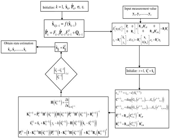
Figure 1.
Flow diagram for the MCCEKF-NR.
In order to improve the shortcomings of the KF and estimate the noise covariance matrices, an extended KF can be employed as the filter with noise-adaptivity technique. The adaptive approach has the advantage of maintaining covariance in line with actual performance. The covariance-matching and correlation methods use the innovation sequences to estimate the noise covariances. Making the residual’s real covariance value compatible with its theoretical value is the fundamental tenet of the covariance-matching strategy.
It is assumed that the mean of the process and measurement noise terms is zero, at which point the anticipated state estimate and measurement residual are assessed. Other than that, the non-additive noise formulation is applied using the same methodology as the additive noise EKF. By repeatedly changing the Taylor expansion’s center point, the iterated extended Kalman filter enhances the extended Kalman filter’s linearization [35]. At the expense of higher processing demands, this lowers the linearization error. The designer can adjust the scalar that parameterizes the extra term to balance the mean-square-error and peak error performance criterion.
The procedures involved in computing the EKF based on the maximum correntropy criterion with nonlinear regression (MCCEKF-NR) is presented below:
- (1)
- Let us first consider a kernel bandwidth , and with small positive value for the error tolerance. Then initialize , ;
- (2)
- Then predict, ,
- (3)
- Updating,If thenOtherwise
- (4)
- Iteration loop: Calculation of using the following steps:
- i.
- ii.
- iii.
- iv.
- v.
- vi.
- vii.
- viii.
- (5)
- If then go to step 6; otherwise, set , and go back to step 4.
- (6)
- Then, set , and go back to step 2.
It is worth noting that the above algorithm for MCCEKF-NR supports a nonlinear regression concept for improving the estimated accuracy.
3. Results and Discussion
Figure 1 represents the flow diagram of the MCCEKF with a nonlinear regression process and the algorithm is summerized above. The simulation analyses aim to verify the suggested strategy’s efficacy in dealing with the effects of a time-varying satellite signal quality by comparing its performance to that of the traditional GPS navigation procedure. The commercially available software programs, Satellite Navigation (SatNav) Toolbox [36] and Inertial Navigation System (INS) Toolbox [37] with MATLAB® codes are used for this study. The INS Toolbox is utilized to generate the vehicle’s trajectory, while the SatNav Toolbox is employed to generate the satellite orbits and pseudoranges. To investigate the estimation performance of different types of filters for navigation, filters are designed, including EKF, MCCEKF, MCCEKF-NR, and Mixture-LRMCCEKF, among others.
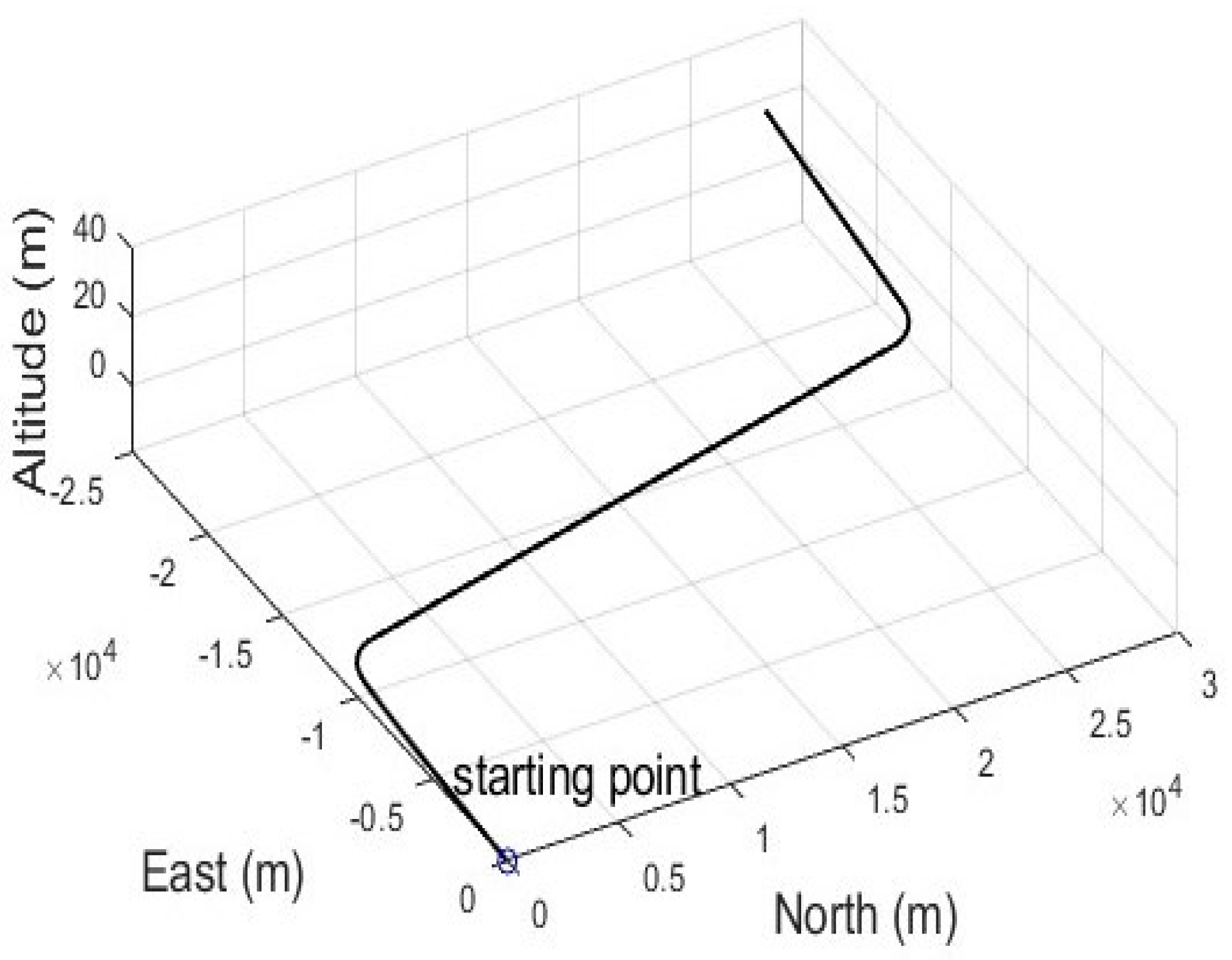
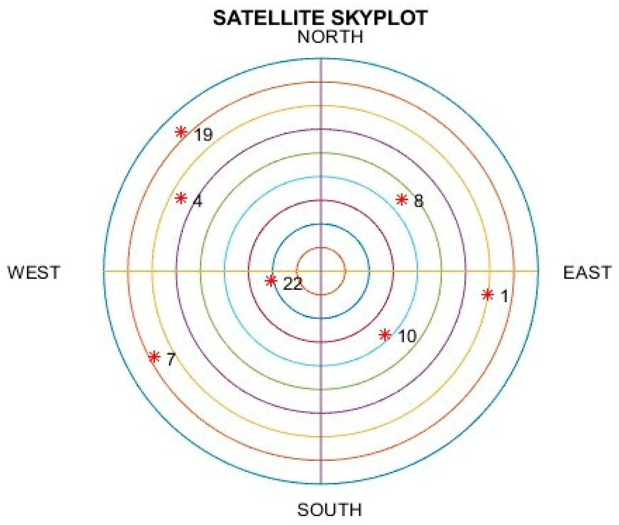
Figure 2 exhibits the test trajectory from the simulation. Seven GPS satellites (marked in red color dots) with the GPS ID number may be reached, as shown in Figure 3. The related Geometry Dilution of Precision (GDOP) is approximately 2.4, which ensures that the positional measurement precision is accurate due to the proper navigation satellite geometry. We concentrated on examining the location errors brought about by pseudorange entities, and these represent the caliber of the measurement model within the filters. The simulated vehicle is situated nearly 100 m above the earth’s surface.

Figure 2.
The test trajectory for the simulated vehicle.
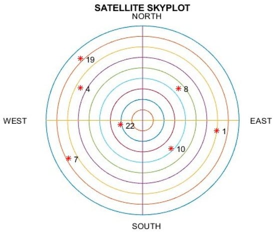
Figure 3.
The skyplot for satellite location.
To evaluate the functionality concerning the outlier level of multipath interruptions, the randomly generated inaccuracies are purposely included in the GPS pseudorange observation data while the vehicle is moving. The ionospheric delay, tropospheric delay, multipath, and receiver noise were the error factors that distorted the GPS observables. Furthermore, most errors were avoided by assuming that the differential GPS (DGPS) mode was used. A Gaussian sequence with a zero median and unity variance was assumed to represent the error caused by the thermal noise in the receiver. In addition, some additional deliberately created and randomly generated situations were used to assess the effectiveness of the outlier kind of multipath interference. These events introduce inaccurate data that interfere with the GPS sensor’s ability to precisely position as a whole. In this study, different types of error calculations were carried out to obtain an error-free signal for GPS navigation; for example, the general error, mean error (ME), mean square error (MSE), root mean square error (RMSE), root mean square error (RMSE), and the average root mean square error (ARMSE) at each time step are all measured statistically during the 100 Monte Carlo simulations. The following are the calculation formulas:
where M and K denote the total number of Monte Carlo runs and total time steps in a single Monte Carlo run, respectively.
In the current scenario, the position–velocity (PV) model suitable for low/medium dynamic motion is adopted from [37]. With a sampling period of ∆T, the model is obtained using the rectangle integral, and data are recorded from the radar every 1 s.
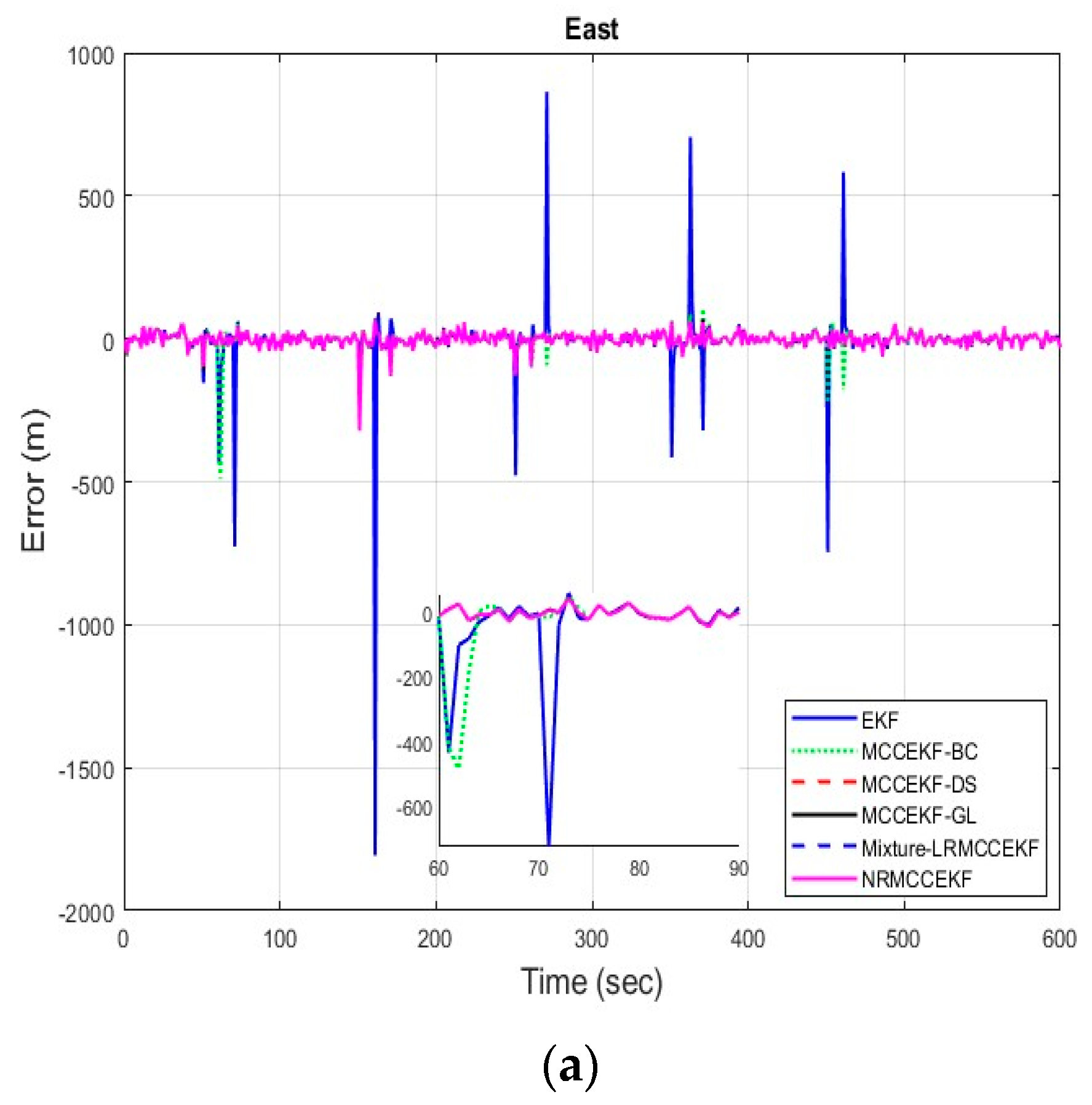
The six different filtering approaches’ precision in terms of errors for different positioning comparisons, such as EKF, MCCEKF-BC, MCCEKF-DS, MCCEKF-GL, MCCEKF-NR, and Mixture-LRMCCEKF, are presented in Figure 4a–c. It is worth mentioning that the MCC is considered for all the EKF-based approaches in this study; however, nonlinear regression with MCC is considered for MCCEKF-NR, and MCC with a mixture of Gaussian noises is considered for Mixture-LRMCCEKF. The noise strength changes with respect to time appeared more in the case of EKF as compared to other filters. However, the EKF can enhance performance even further by considering the MCC. According to a different perspective, the MCC mechanism helped the EKF’s noise variance adaptability performance. The MCC-based nonlinear regression method offers superior computational efficiency along with comparable positioning accuracy when compared to MCC-based EKFs. Moreover, with only a slight increase in execution time over Mixture-LRMCCEKF, the MCCEKF-NR method offers the best positioning accuracy among the approaches.

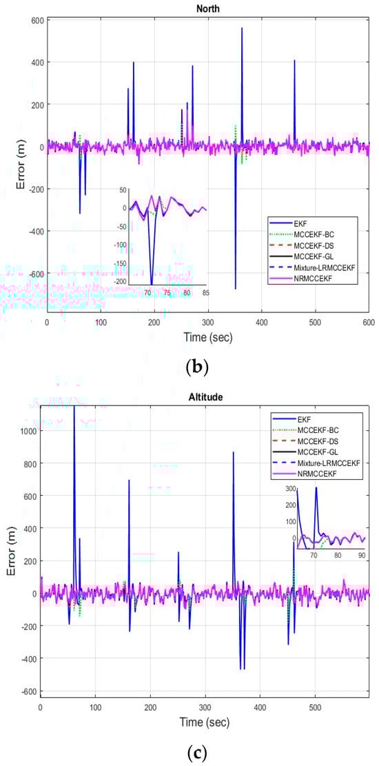
Figure 4.
The error for different MCCEKF with respect to different positions: (a) east, (b) north, and (c) altitude.
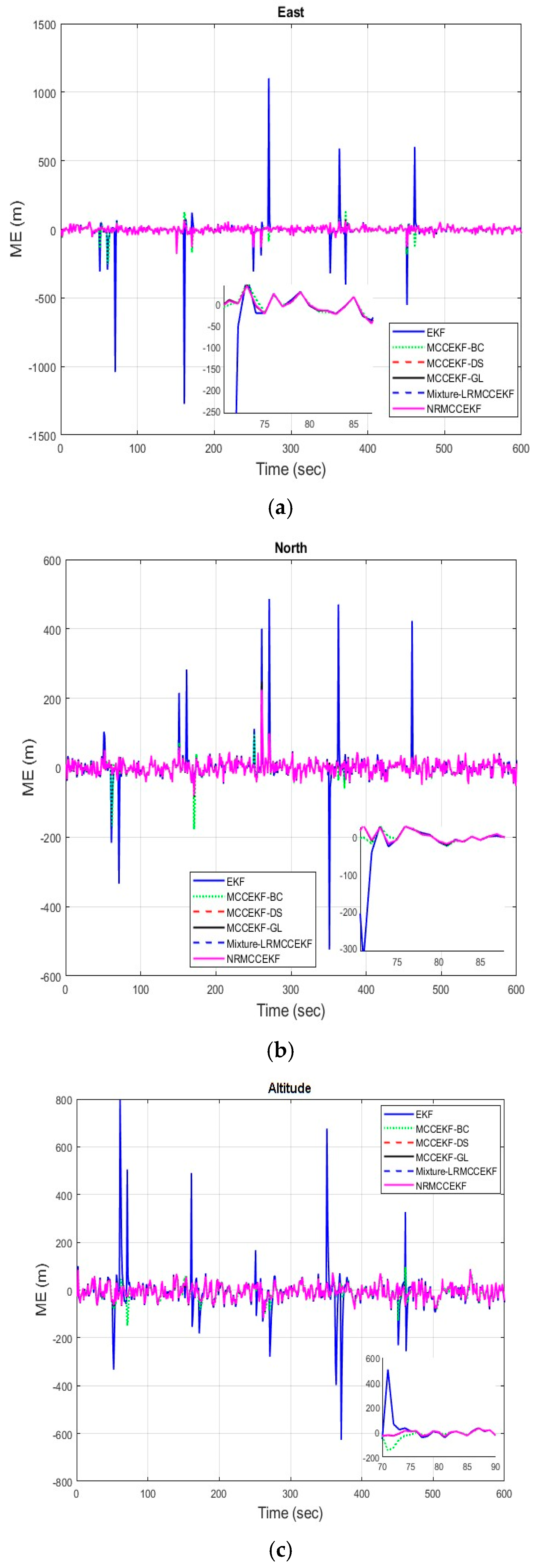
The six different filtering approaches’ precision in terms of mean errors for different positioning comparisons, such as EKF, MCCEKF-BC, MCCEKF-DS, MCCEKF-GL, MCCEKF-NR, and Mixture-LRMCCEKF are presented in Figure 5a–c. The performance comparisons for different algorithms are shown in Table 1 for different positions in terms of MEs, which reveals that Mixture-LRMCCEKF and MCCEKF-NR offer the best positioning accuracy among the approaches.
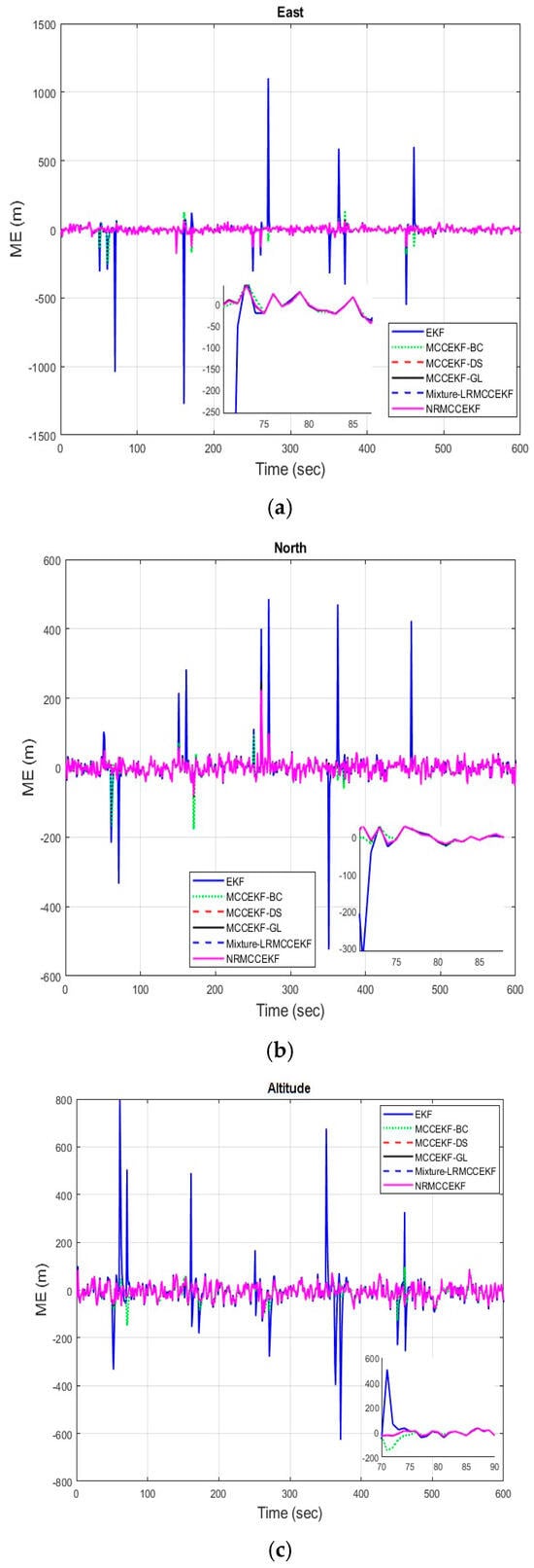
Figure 5.
The minimum error (ME) for different MCCEKF with respect to different positions: (a) east, (b) north, and (c) altitude.

Table 1.
The performance comparison in terms of mean errors (MEs) for different filters with respect to different positions.
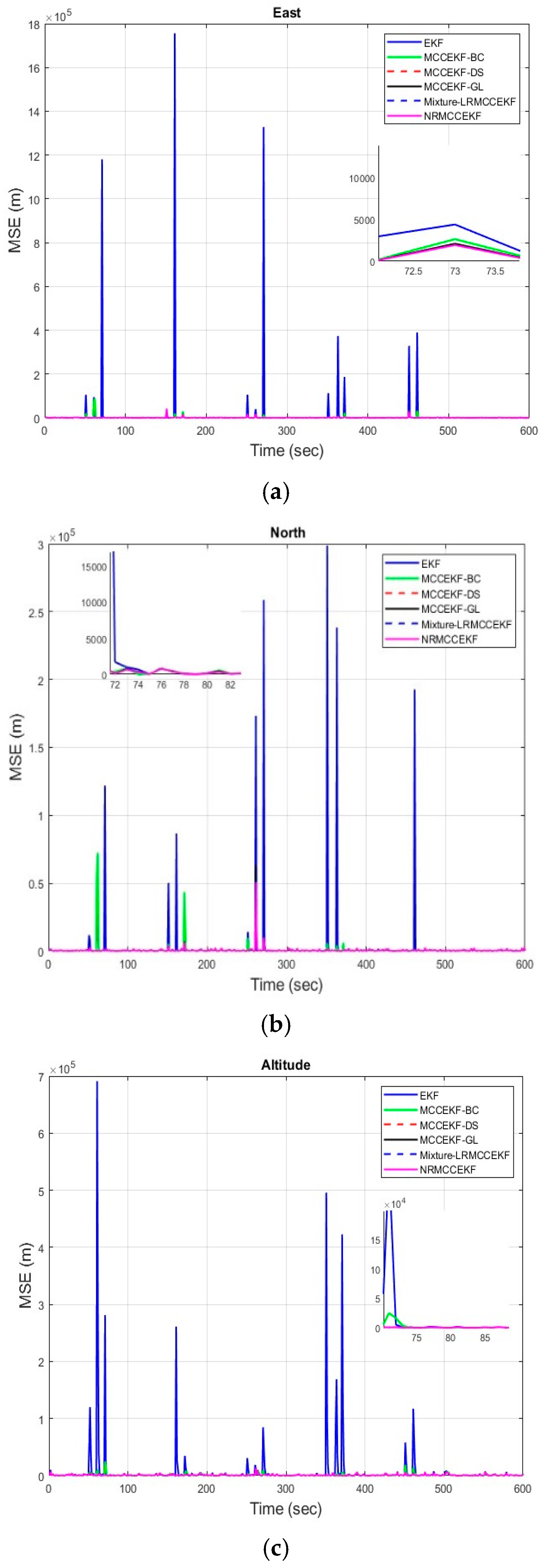
The six different filtering approaches’ precision in terms of mean square errors for different positioning comparisons, such as EKF, MCCEKF-BC, MCCEKF-DS, MCCEKF-GL, MCCEKF-NR, and Mixture-LRMCCEKF are presented in Figure 6a–c. The performance comparison for different algorithms is shown in Table 2, which reveals that Mixture-LRMCCEKF and MCCEKF-NR offer the best positioning accuracy among the approaches in terms of MSE.
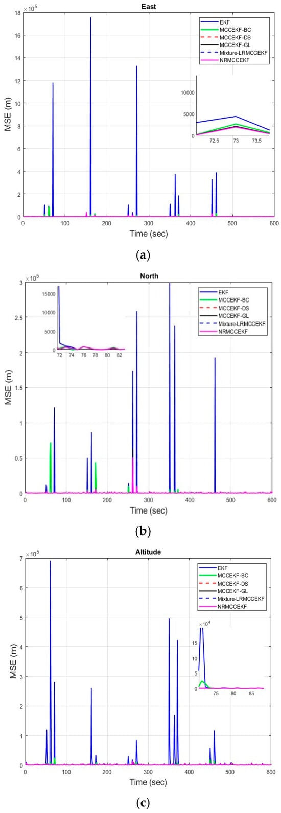
Figure 6.
The mean square error (MSE) for different MCCEKF with respect to different positions: (a) east, (b) north, and (c) altitude.
Table 2.
The performance comparison in terms of mean square errors (MSEs) for different filters with respect to different positions.
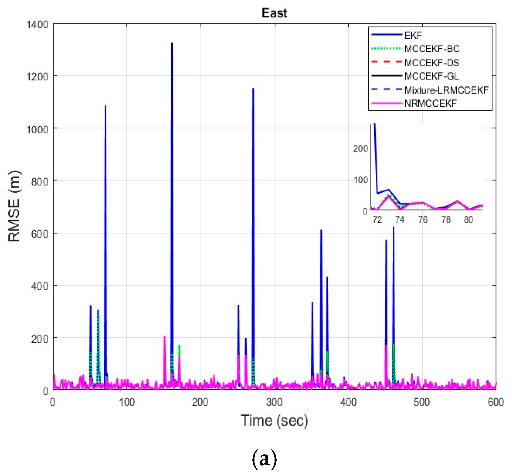
The six different filtering approaches’ precision in terms of root mean square errors for different positioning comparisons, such as EKF, MCCEKF-BC, MCCEKF-DS, MCCEKF-GL, MCCEKF-NR, and Mixture-LRMCCEKF, are presented in Figure 7a–c. The performance comparison for different algorithms is shown in Table 3, which reveals that Mixture-LRMCCEKF and NRMCCEKF offer the best positioning accuracy among the approaches in terms of RMSEs. In the meantime, MCCEKF-NR performs better than the EKF and the other MCCEKFs studied here, and estimates more accurately than the Mixture-LRMCCEKF. Furthermore, it is worth noting that the fixed-point algorithms in Mixture-LRMCCEKF and MCCEKF-NR are based on the iterative EKF converging to the most ideal result for the application in the GPS satellite navigations.
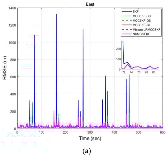
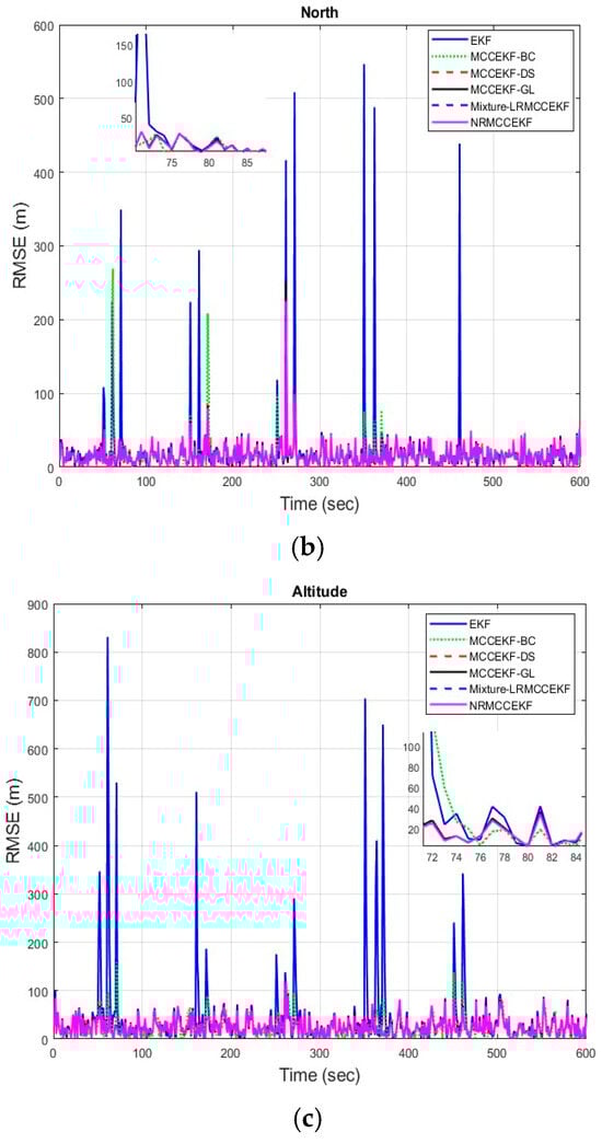
Figure 7.
The root mean square error (RMSE) for different MCCEKF with respect to different positions: (a) east, (b) north, and (c) altitude.
Table 3.
The performance comparison in terms of root mean square errors (RMSEs) for different filters with respect to different positions.
4. Conclusions
This paper introduces an extended Kalman filter based on the maximum mixture correntropy criterion with nonlinear regression (MCCEKF-NR) for GPS navigation and positioning applications. The mixture correntropy was extended with the original correntropy by combining the kernel functions with EKF, and integrating them into a nonlinear regression-based filtering algorithm technique. The resulting filter was designed from the corresponding cost function, which offers better robustness and filtering performance than typical correntropy-based filters and also other types of EKF-based filters. By repeatedly altering the Taylor expansion’s center point, the iterated extended Kalman filter enhances the extended Kalman filter’s linearization. Although more processing power is needed, the linearization error is decreased.
Although there is no set standard for choosing the kernel width in the original correntropy, it has a big influence on the system as a whole. Thus, more flexibility is possible when employing the MCC, which integrates the kernel bandwidth, including distinct algorithm techniques. Using the fixed-point iteration for Gaussian and mixed-Gaussian noises ensures effective performance in the presence of outliers. This method avoids problems such as divergence resulting from extremely large or very small kernel bandwidth when the outliers are present. The effect of the ratio between the kernel bandwidth and the filter performance also plays a vital role in choosing an appropriate kernel bandwidth. The proposed MCCEKF-NR and Mixture-LRMCCEKF can achieve better performance as compared to the different MCCEKF techniques for a suitable kernel bandwidth; this has been verified from the simulation results. Additionally, we implemented the linear and nonlinear regression-based algorithms for the MCCEKF to improve the estimation accuracy by considering the iterated EKF (IEKF) for the GPS navigation.
Further, the simulation tests for GPS navigation were included to demonstrate the efficiency. The findings indicate that the adaptive regression filtering algorithm based on the kernel entropy principle exhibits a discernible enhancement in navigation accuracy when interconnecting with the traditional techniques. Consequently, it shows promising potential as a substitute for the GPS navigation processor, particularly when dealing with observables that exhibit mixed-Gaussian errors. We demonstrate our findings in four different methods of error calculation for Gaussian and mixed-Gaussian noise environments. Performance comparisons were conducted for a number of techniques, such as EKF, MCCEKF-BC, MCCEKF-DS, MCCEKF-GL, MCCEKF-NR, and Mixture-LRMCCEKF. The kernel entropy-based MCCEKF with nonlinear regression algorithm showed encouraging results in terms of improving navigational accuracy. Moreover, this work can be extended to design MCCEKF-based filters for state-constrained processes, and systems with continuous networks.
Author Contributions
Conceptualization, A.B.; methodology, A.B.; software, A.B.; validation, A.B.; writing original draft preparation, A.B.; writing review and editing, A.B. and D.-J.J.; supervision, D.-J.J. All authors have read and agreed to the published version of the manuscript.
Funding
The author gratefully acknowledges the support of the National Science and Technology Council, Taiwan under grant numbers NSTC 112-2221-E-019-030 and NSTC 112- 2811-E-019-004.
Institutional Review Board Statement
Not applicable.
Informed Consent Statement
Not applicable.
Data Availability Statement
Data are contained within the article.
Conflicts of Interest
The authors declare no conflicts of interest.
References
- Anderson, B.D.; Moore, J.B. Optimal Filtering; Courier Corporation: North Chelmsford, MA, USA, 2005. [Google Scholar]
- Bar-Shalom, Y.B.; Li, X.R.; Kirubarajan, T. Estimation, Tracking and Navigation: Theory, Algorithms and Software; Wiley: Hoboken, NJ, USA, 2001. [Google Scholar]
- Huang, Y.; Zhang, Y.; Shi, P.; Wu, Z.; Qian, J.; Chambers, J.A. Robust Kalman filters based on Gaussian scale mixture distributions with application to target tracking. IEEE Trans. Syst. Man Cybern. Syst. 2017, 49, 2082–2096. [Google Scholar] [CrossRef]
- Abdelrahman, M.; Park, S.Y. Sigma-point Kalman filtering for spacecraft attitude and rate estimation using magnetometer measurements. IEEE Trans. Aerosp. Electron. Syst. 2011, 47, 1401–1415. [Google Scholar] [CrossRef]
- Liu, X.; Ren, Z.; Lyu, H.; Jiang, Z.; Ren, P.; Chen, B. Linear and nonlinear regression-based maximum correntropy extended Kalman filtering. IEEE Trans. Syst. Man Cybern. Syst. 2019, 51, 3093–3102. [Google Scholar] [CrossRef]
- Wan, E.A.; Van Der Merwe, R. The unscented Kalman filter. In Kalman Filtering and Neural Networks; Wiley: Hoboken, NJ, USA, 2001; pp. 221–280. [Google Scholar]
- Arasaratnam, I.; Haykin, S. Cubature kalman filters. IEEE Trans. Autom. Control 2009, 54, 1254–1269. [Google Scholar] [CrossRef]
- Ito, K.; Xiong, K. Gaussian filters for nonlinear filtering problems. IEEE Trans. Autom. Control 2000, 45, 910–927. [Google Scholar] [CrossRef]
- Huang, Y.; Zhang, Y.; Zhao, Y.; Shi, P.; Chambers, J.A. A novel outlier-robust Kalman filtering framework based on statistical similarity measure. IEEE Trans. Autom. Control 2020, 66, 2677–2692. [Google Scholar] [CrossRef]
- Karlgaard, C.D. Nonlinear regression Huber–Kalman filtering and fixed-interval smoothing. J. Guid. Control Dyn. 2015, 38, 322–330. [Google Scholar] [CrossRef]
- Huang, Y.; Zhang, Y.; Li, N.; Wu, Z.; Chambers, J.A. A novel robust student’s t-based Kalman filter. IEEE Trans. Aerosp. Electron. Syst. 2017, 53, 1545–1554. [Google Scholar] [CrossRef]
- Roth, M.; Özkan, E.; Gustafsson, F.A. Student’s t filter for heavy tailed process and measurement noise. In Proceedings of the 2013 IEEE International Conference on Acoustics, Speech and Signal Processing, Vancouver, BC, Canada, 26–31 May 2013; pp. 5770–5774. [Google Scholar]
- Huang, H.; Zhang, H. Student’s t-Kernel-Based Maximum Correntropy Kalman Filter. Sensors 2022, 22, 1683. [Google Scholar] [CrossRef]
- Chen, W.; Li, Z.; Chen, Z.; Sun, Y.; Liu, Y. Multiple similarity measure-based maximum correntropy criterion Kalman filter with adaptive kernel width for GPS/INS integration navigation. Measurement 2023, 222, 113666. [Google Scholar] [CrossRef]
- Lu, C.; Zhang, Y.; Ge, Q. Kalman filter based on multiple scaled multivariate skew normal variance mean mixture distributions with application to target tracking. IEEE Trans. Circuits Syst. II Express Briefs 2020, 68, 802–806. [Google Scholar] [CrossRef]
- Liu, W.; Pokharel, P.P.; Principe, J.C. Correntropy: Properties and applications in non-Gaussian signal processing. IEEE Trans. Signal Process. 2007, 55, 5286–5298. [Google Scholar] [CrossRef]
- Principe, J.C. Information Theoretic Learning: Renyi’s Entropy and Kernel Perspectives; Springer Science & Business Media: New York, NY, USA, 2010. [Google Scholar]
- Chen, X.; Yang, J.; Liang, J.; Ye, Q. Recursive robust least squares support vector regression based on maximum correntropy criterion. Neurocomputing 2012, 97, 63–73. [Google Scholar] [CrossRef]
- Wang, D.; Zhang, H.; Huang, H.; Ge, B. A redundant measurement-based maximum correntropy extended Kalman filter for the noise covariance estimation in INS/GNSS integration. Remote Sens. 2023, 15, 2430. [Google Scholar] [CrossRef]
- Shi, L.; Lin, Y. Convex combination of adaptive filters under the maximum correntropy criterion in impulsive interference. IEEE Signal Process. Lett. 2014, 21, 1385–1388. [Google Scholar] [CrossRef]
- Ogunfunmi, T.; Paul, T. The quarternion maximum correntropy algorithm. IEEE Trans. Circuits Syst. II Express Briefs 2015, 62, 598–602. [Google Scholar] [CrossRef]
- Wang, G.; Li, N.; Zhang, Y. Maximum correntropy unscented Kalman and information filters for non-Gaussian measurement noise. J. Frankl. Inst. 2017, 354, 8659–8677. [Google Scholar] [CrossRef]
- He, R.; Hu, B.; Yuan, X.; Wang, L. Robust Recognition via Information Theoretic Learning; Springer International Publishing: Berlin/Heidelberg, Germany, 2014. [Google Scholar]
- Zhao, S.; Chen, B.; Principe, J.C. Kernel adaptive filtering with maximum correntropy criterion. In Proceedings of the 2011 International Joint Conference on Neural Networks, San Jose, CA, USA, 31 July–5 August 2011; pp. 2012–2017. [Google Scholar]
- Wu, Z.; Shi, J.; Zhang, X.; Ma, W.; Chen, B. Senior Member, IEEE. Kernel recursive maximum correntropy. Signal Process. 2015, 117, 11–16. [Google Scholar] [CrossRef]
- Bao, R.J.; Rong, H.J.; Angelov, P.P.; Chen, B.; Wong, P.K. Correntropy-based evolving fuzzy neural system. IEEE Trans. Fuzzy Syst. 2017, 26, 1324–1338. [Google Scholar] [CrossRef]
- Ma, W.; Zheng, D.; Li, Y.; Zhang, Z.; Chen, B. Bias-compensated normalized maximum correntropy criterion algorithm for system identification with noisy input. Signal Process. 2018, 152, 160–164. [Google Scholar] [CrossRef]
- Cinar, G.T.; Príncipe, J.C. Hidden state estimation using the correntropy filter with fixed point update and adaptive kernel size. In Proceedings of the 2012 International Joint Conference on Neural Networks (IJCNN), Brisbane, QLD, Australia, 10–15 June 2012; pp. 1–6. [Google Scholar]
- Chen, B.; Liu, X.; Zhao, H.; Principe, J.C. Maximum correntropy Kalman filter. Automatica 2017, 76, 70–77. [Google Scholar] [CrossRef]
- Jing, H.; Gao, Y.; Shahbeigi, S.; Dianati, M. Integrity monitoring of GNSS/INS based positioning systems for autonomous vehicles: State-of-the-art and open challenges. IEEE Trans. Intell. Transp. Syst. 2022, 23, 14166–14187. [Google Scholar] [CrossRef]
- Liu, X.; Qu, H.; Zhao, J.; Chen, B. Extended Kalman filter under maximum correntropy criterion. In Proceedings of the 2016 International Joint Conference on Neural Networks (IJCNN), Vancouver, BC, Canada, 24–29 July 2016; pp. 1733–1737. [Google Scholar]
- Dang, L.; Huang, Y.; Zhang, Y.; Chen, B. Multi-kernel correntropy based extended Kalman filtering for state-of-charge estimation. ISA Trans. 2022, 129, 271–283. [Google Scholar] [CrossRef] [PubMed]
- Jwo, D.J.; Cho, T.S.; Biswal, A. Geometric Insights into the Multivariate Gaussian Distribution and Its Entropy and Mutual Information. Entropy 2023, 25, 1177. [Google Scholar] [CrossRef] [PubMed]
- Simon, D. Optimal State Estimation: Kalman, H Infinity, and Nonlinear Approaches; John Wiley & Sons: Hoboken, NJ, USA, 2006. [Google Scholar]
- Brown, R.G.; Hwang, P.Y.C. Introduction to Random Signals and Applied Kalman Filtering; John Wiley & Sons: New York, NY, USA, 1997. [Google Scholar]
- GPSoft LLC. Satellite Navigation Toolbox 3.0 User’s Guide; GPSoft LLC: Athens, OH, USA, 2003. [Google Scholar]
- GPSoft LLC. Inertial Navigation System Toolbox 3.0 User’s Guide; GPSoft LLC: Athens, OH, USA, 2007. [Google Scholar]


Disclaimer/Publisher’s Note: The statements, opinions and data contained in all publications are solely those of the individual author(s) and contributor(s) and not of MDPI and/or the editor(s). MDPI and/or the editor(s) disclaim responsibility for any injury to people or property resulting from any ideas, methods, instructions or products referred to in the content. |
© 2024 by the authors. Licensee MDPI, Basel, Switzerland. This article is an open access article distributed under the terms and conditions of the Creative Commons Attribution (CC BY) license (https://creativecommons.org/licenses/by/4.0/).