MILP-Based Approach for High-Altitude Region Pavement Maintenance Decision Optimization

Abstract

Affected by climatic factors (e.g., low temperature and intense ultraviolet radiation), high-altitude regions experience numerous pavement diseases, which compromise driving safety and negatively impact user travel experience. Timely planning and execution of pavement maintenance are particularly critical. In this paper, considering the characteristics of pavement maintenance in high-altitude regions (e.g., volatility of traffic volume, seasonality of maintenance timing, and fragility of the ecological environment), we aim to derive optimal monthly maintenance plans. We develop a multi-objective nonlinear optimization model that comprehensively accounts for minimizing maintenance costs, affected traffic volume and carbon emissions, and maximizing pavement maintenance effectiveness. Utilizing linearization methods, the model is reconstructed into a typical mixed-integer linear programming (MILP) model, enabling it to be solved directly using conventional solvers. We consider five types of decision strategies to reflect the preferences of different decision-makers. Given the uncertainty of maintenance costs, we also utilize the robust optimization method based on the acceptable objective variation range (AOVR) to construct a robust optimization model and discuss the characteristics of optimistic, robust, and pessimistic solutions. The results suggest that different decision strategies show differences in the indicators of maintenance costs, affected traffic volume, carbon emissions, and pavement performance. When multiple decision objectives are comprehensively considered, the indicators are between the maximum and minimum values, which can effectively balance the decision needs of maintenance effectiveness, maintenance timing, and environmental protection. The number of maintenance workers, the requirement of the minimum pavement condition index (PCI), and the annual budget influence the maintenance planning. The obtained robust solution can somewhat overcome the conservative nature of the pessimistic solution. The method proposed in this paper helps address the complexities of pavement maintenance decisions in high-altitude regions and provides guidance for pavement maintenance decisions in such areas.

1. Introduction

Transportation plays a crucial role in people’s work and life, influencing the development of society and economy. Roads serve as the foundation for road traffic vehicles, with pavements being a critical component of road infrastructure. Therefore, it is essential to ensure that their performance meets usage requirements, guaranteeing the safety of vehicle operation and the travel experience of users. Due to the limitations of the full life cycle, pavement performance degrades during use. Road maintenance is the primary method to improve pavement performance [1,2,3], and timely and effective maintenance is of significant importance in maintaining good pavement conditions. Road maintenance planning involves numerous issues, including maintenance targets, maintenance timing, maintenance approaches, costs, impacts of maintenance, and expected maintenance effectiveness. In fact, road maintenance decision-making is not only a focus for researchers but also of interest to road management authorities.

The climatic characteristics of high-altitude areas, such as low temperatures, frequent rain and snow, and intense ultraviolet radiation, accelerate pavement aging and induce various pavement diseases, severely affecting pavement lifespan [4,5]. Additionally, the climate in high-altitude regions influences pavement maintenance, particularly the planning of preventive pavement maintenance. For example, some road segments may be challenging to maintain due to accumulated snow. Therefore, studying pavement maintenance decisions in the areas and determining scientifically reasonable maintenance plans can not only help extend the pavement lifespan but also contribute to ensuring road service levels, thereby providing robust support for social and economic activities in such regions.

1.1. Literature Review

In the previous literature, He et al. [1], Pourgholamali et al. [3], and Xu et al. [6] have reviewed some work on pavement maintenance decisions. This paper further reviews these two perspectives, project-level and network-level [7], and Table 1 intuitively summarizes the characteristics described in some related literature.

Project-level pavement maintenance decision-making primarily focuses on developing maintenance plans, optimizing budgets, and evaluating maintenance effects for a specific road segment. Detailed data are used to formulate a specific maintenance plan, emphasizing maximizing service levels and lifespan of the segment under limited resources. Yu et al. [8] discussed the multi-objective optimization of project-level pavement maintenance plans, constructing an optimization model integrating pavement performance, costs, and environmental impacts, and designing the corresponding genetic algorithm (GA). Wang et al. [9] focused on the integrated optimization of timing and strategies for preventive maintenance of asphalt pavements based on periods, constructing an integrated optimization approach for preventive maintenance timing and strategies based on the reconstructed data envelopment analysis (DEA). Li et al. [10] proposed a preventive maintenance decision method for asphalt pavements considering multiple damage characteristics by constructing a BP neural network model that combines dominant damage and overall damage. Zhang et al. [11] addressed the optimization of pavement maintenance decisions under dual constraints of funding and effectiveness, proposing a multi-annual project-level maintenance planning decision process.

The project-level pavement maintenance decision-making is relatively meticulous, but this approach cannot carry out a comprehensive decision at the network level, which is a practical demand. Network-level pavement maintenance decisions can compensate for this shortcoming, involving multiple road systems within a region. The primary goal of the network-level maintenance decision is to determine the road segments within the network that need maintenance and allocate appropriate maintenance methods and timings. Mahmood et al. [12] discussed the optimization of multi-objective pavement maintenance decision plans, proposing a parameter-free discrete particle swarm algorithm. He et al. [1] constructed an optimization model considering the needs of the government, highway agencies, contractors, and common users for pavement maintenance and rehabilitation management systems. Sun et al. [13] discussed the multi-objective optimization problem of network-level pavement maintenance and rehabilitation programming, constructing an integer programming model to optimize road conditions, user disruption costs, and agency costs, and proposing a Pareto-based optimal trade-off method. Chen et al. [14] combined the generalized differential evolution 3 (GDE3) algorithm, life cycle assessment (LCA), and life cycle cost analysis (LCCA) to construct a multi-objective decision model for highway network maintenance. Lee et al. [15] discussed the optimal pavement management strategy to reduce greenhouse gas emissions under budget constraints, constructed an optimization model considering budget constraints and minimizing greenhouse gas emissions, and designed a solution algorithm based on Lagrangian relaxation and dynamic programming. Elhadidy et al. [16] constructed a performance prediction model based on the Markov chain model, focusing on maximizing the overall condition of the road network while minimizing maintenance and renovation costs. Fani et al. [17] discussed the optimization of pavement maintenance and rehabilitation planning under budget and pavement deterioration uncertainties and constructed a multi-stage stochastic mixed-integer programming model. Lee et al. [18] constructed a multi-dimensional pavement segment status and a heterogeneous management activities model considering greenhouse gas emissions, aiming to minimize life cycle costs for pavement maintenance. Li et al. [19] proposed a multi-stage dynamic programming optimal decision model based on network traffic flow equilibrium to minimize maintenance and user costs. Meng et al. [20] discussed a multi-objective optimization model for multi-annual network-level pavement maintenance planning based on user travel time costs and vehicle operating costs and designed the non-dominated sorting genetic algorithm (i.e., NSGA-III) with a wide reference point. Fan et al. [21] proposed an optimization method for managing pavement maintenance and rehabilitation projects under budget uncertainty.

1.2. The Focus of This Study

Pavement maintenance in high-altitude regions has some unique characteristics that make the maintenance work more complex and challenging compared with other regions. First, taking the Tibet Autonomous Region of China (Tibet, for short) as an example, the traffic flow in Tibet has obvious seasonal characteristics. During the peak tourist seasons, such as summer and autumn, the number of tourists is high, resulting in heavy traffic flow. In winter and early spring, due to cold and extreme weather conditions, the number of tourists is low, leading to reduced traffic flow [22]. This seasonal variation in traffic flow needs to be fully considered in maintenance planning to ensure that roads can withstand high traffic pressure during peak tourist seasons while minimizing disruption to traffic services. Second, the climatic conditions in high-altitude regions determine the seasonality of road maintenance work. Due to the low temperatures in winter, some road segments experience ice and snow, leading to harsh conditions that are unsuitable for large-scale maintenance activities. Therefore, it is more appropriate to carry out pavement maintenance work in warmer seasons, particularly summer and autumn [23]. This requires reasonable planning of maintenance work to minimize the impact of adverse weather on pavement maintenance and ensure maintenance quality and pavement technical condition. Furthermore, the ecological environment in Tibet is fragile, requiring environmental considerations in maintenance planning to minimize the impact on the ecosystem [24]. Additionally, due to the location of Tibet, the prices of maintenance materials are uncertain, and maintenance costs are generally high [25].

Some previous studies have considered reducing costs and carbon emissions during pavement maintenance, while others have considered budget uncertainties. However, previous methods did not fully address the maintenance decision needs of high-altitude regions and cannot be directly applied to such areas. To the best of our knowledge, previous studies have focused on annual maintenance plans without considering monthly maintenance plans. Additionally, most studies did not consider the duration of the maintenance process or manpower constraints. Moreover, no research has focused on the impact of unit area maintenance cost variations on maintenance plans, especially the corresponding robust maintenance plans. Inspired by the above background, this paper uses constraints such as manpower, maintenance months, budget, maintenance frequency, and maintenance approaches to analyze optimization objectives from multiple perspectives and propose methods for obtaining maintenance plans and robust maintenance plans. Specifically, the contributions of this paper are as follows:

Table 1. Summary of the literature studies on pavement maintenance.

Literature	Object Characteristic	Optimization Objective	Model Type	Solution Approach
Yu et al. [8]	Project-level; considering greenhouse gas emissions and budget constraints; meeting pavement condition requirements	Greenhouse gas emissions, maintenance costs, pavement condition	Multi-objective nonlinear optimization	Genetic algorithm
Zhang et al. [11]	Project-level; constrained budget; meeting pavement condition requirements	Pavement condition	Flowchart	Heuristic algorithm
Mahmood et al. [12]	Project-level; meeting pavement condition requirements	Maintenance costs, pavement condition	Multi-objective nonlinear optimization	Improved particle swarm algorithm
He and Sun [1]	Network-level; different decision-makers	Benefits for different decision-makers	Mixed-integer programming	Lingo
Sun et al. [13]	Network-level; different decision-makers; Pareto optimal solution	Maintenance costs, pavement condition, and environmental impact	Mixed-integer linear programming	Cplex
Chen and Wang [14]	Network-level; multiple pavement condition indicators	Maintenance costs, carbon emissions, and energy consumption	Multi-objective optimization	Generalized differential evolution algorithm
Lee and Madanat [15]	Network-level; single or multiple budget constraints	Greenhouse gas emission	Single-objective optimization	Lagrangian relaxation
Elhadidy et al. [16]	Network-level; Pareto optimal solution	Maintenance costs, pavement condition	Markov-chain, multi-objective optimization	Genetic algorithm-based procedure
Fani et al. [17]	Network-level; considering the uncertainty of pavement deterioration and budget deterioration and budget	Pavement condition	Multi-stage stochastic mixed-integer programming	GAMS
Lee et al. [18]	Network-level; constrained greenhouse gas emissions	Maintenance costs	Single-objective nonlinear	Two-stage algorithm
Li et al. [19]	Network-level; considering dynamic traffic distribution	Maintenance costs, user costs, pavement residual asset value	Multi-stage dynamic programming	Heuristic iterative algorithm
FAN and Feng [21]	Network-level; budget uncertainty	Maintenance effectiveness	Stochastic linear programming	Scenario tree-based heuristic algorithm
This paper	Network-level; high-altitude region pavement maintenance; monthly maintenance plans; robust solution	Maintenance costs, affected traffic volume, carbon emissions, comfort level, maintenance effectiveness	Mixed-integer linear programming	Gurobi

Table 1. Summary of the literature studies on pavement maintenance.

Literature	Object Characteristic	Optimization Objective	Model Type	Solution Approach
Yu et al. [8]	Project-level; considering greenhouse gas emissions and budget constraints; meeting pavement condition requirements	Greenhouse gas emissions, maintenance costs, pavement condition	Multi-objective nonlinear optimization	Genetic algorithm
Zhang et al. [11]	Project-level; constrained budget; meeting pavement condition requirements	Pavement condition	Flowchart	Heuristic algorithm
Mahmood et al. [12]	Project-level; meeting pavement condition requirements	Maintenance costs, pavement condition	Multi-objective nonlinear optimization	Improved particle swarm algorithm
He and Sun [1]	Network-level; different decision-makers	Benefits for different decision-makers	Mixed-integer programming	Lingo
Sun et al. [13]	Network-level; different decision-makers; Pareto optimal solution	Maintenance costs, pavement condition, and environmental impact	Mixed-integer linear programming	Cplex
Chen and Wang [14]	Network-level; multiple pavement condition indicators	Maintenance costs, carbon emissions, and energy consumption	Multi-objective optimization	Generalized differential evolution algorithm
Lee and Madanat [15]	Network-level; single or multiple budget constraints	Greenhouse gas emission	Single-objective optimization	Lagrangian relaxation
Elhadidy et al. [16]	Network-level; Pareto optimal solution	Maintenance costs, pavement condition	Markov-chain, multi-objective optimization	Genetic algorithm-based procedure
Fani et al. [17]	Network-level; considering the uncertainty of pavement deterioration and budget deterioration and budget	Pavement condition	Multi-stage stochastic mixed-integer programming	GAMS
Lee et al. [18]	Network-level; constrained greenhouse gas emissions	Maintenance costs	Single-objective nonlinear	Two-stage algorithm
Li et al. [19]	Network-level; considering dynamic traffic distribution	Maintenance costs, user costs, pavement residual asset value	Multi-stage dynamic programming	Heuristic iterative algorithm
FAN and Feng [21]	Network-level; budget uncertainty	Maintenance effectiveness	Stochastic linear programming	Scenario tree-based heuristic algorithm
This paper	Network-level; high-altitude region pavement maintenance; monthly maintenance plans; robust solution	Maintenance costs, affected traffic volume, carbon emissions, comfort level, maintenance effectiveness	Mixed-integer linear programming	Gurobi

(1)

For the pavement maintenance decision problem in high-altitude regions, this paper proposes an optimization method for pavement maintenance plans. The initial optimization model constructed considers the typical characteristics of pavement maintenance in high-altitude regions (see Section 2) intending to obtain monthly maintenance plans. By combining the proposed linearization method, the initial nonlinear model is reconstructed into a mixed-integer linear programming (MILP) problem. The composition of the model under five types of decision strategies is discussed (see Section 4.2), responding to the decision- makers’ preferences.

(2)

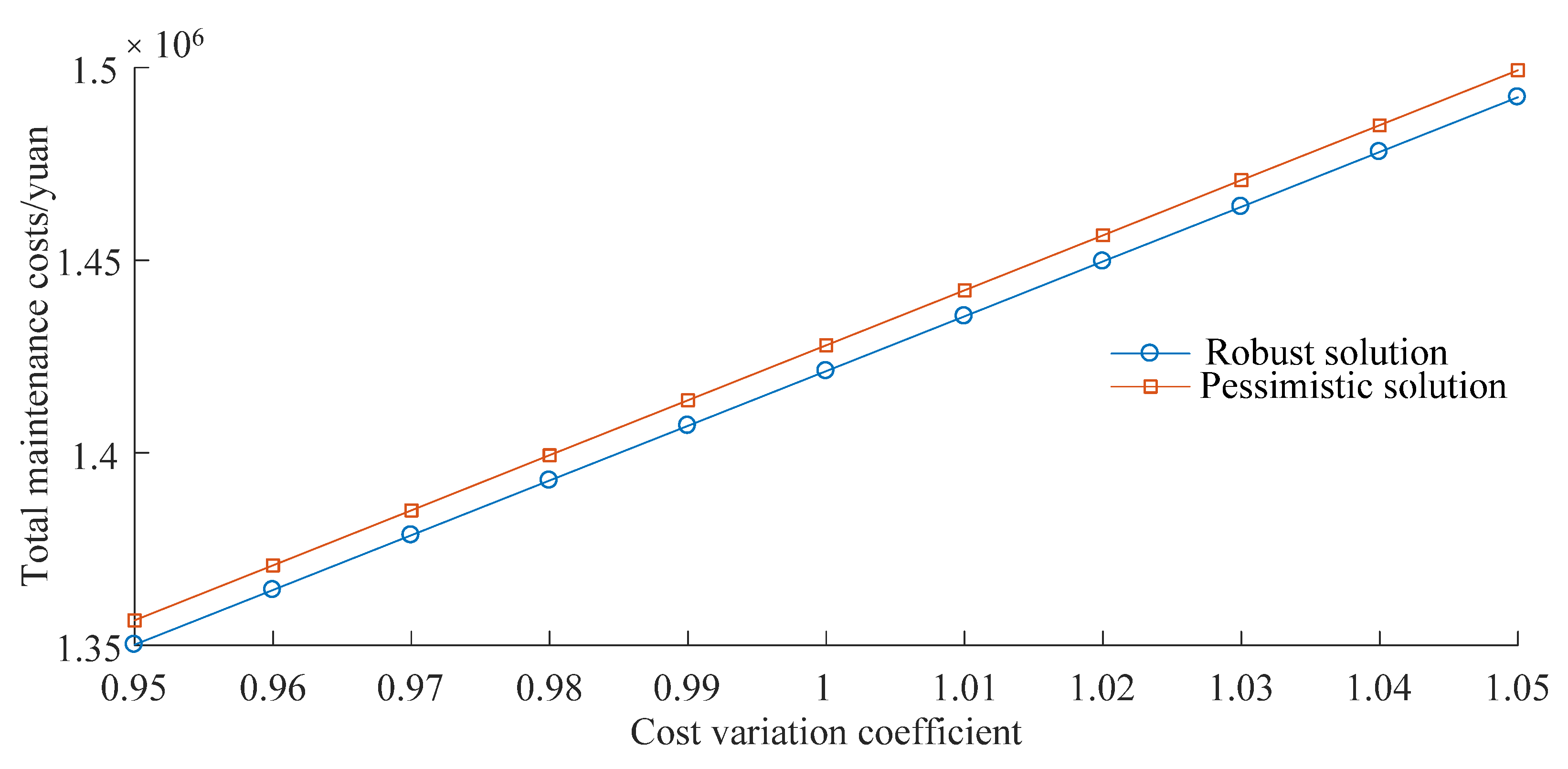
To address the uncertainty of unit maintenance costs, this paper proposes a robust maintenance plan calculation method using a robust optimization method based on the acceptable objective variation range (AOVR). By setting the unit maintenance cost as an interval number, the corresponding optimistic sub-model and pessimistic sub-model are analyzed, and the construction process of the robust optimization model and the process of obtaining robust maintenance plans are discussed.

(3)

Combining a specific network-level pavement maintenance decision problem, a case study analysis is conducted. A maintenance decision problem involving 30 road segments is used to discuss the characteristics of different decision strategies; analyze the impact of the number of maintenance workers, annual budget, and minimum pavement condition index (PCI) requirements on decision plans; and discuss the differences among the robust, pessimistic, and optimistic solutions.

The remainder is given as follows. Section 2 describes the problem addressed in this paper, including the characteristics of pavement maintenance in high-altitude regions. Section 3 details the construction process of the initial pavement maintenance decision model, a nonlinear optimization model, including the definition of symbols, constraints, and the description of the objective function. Section 4 covers the process of reconstructing the initial model into a MILP problem, including five lemmas for converting nonlinear terms to linear terms, methods for converting the multi-objective optimization problem to a single-objective optimization problem, and settings for five types of decision strategies. Section 5 presents a case study for a specific network-level maintenance problem and discusses the different decision strategies and the sensitivity of model parameters. Section 6 focuses on the uncertainty of unit maintenance costs, discussing methods for obtaining robust maintenance plans. Section 7 concludes this paper.

2. Problem Formulation

For roads, high-altitude regions experience harsher climates compared with lower-altitude regions, including factors such as temperature, rain, snow, and ultraviolet radiation. Pavement diseases impact driving safety and user experience, necessitating targeted maintenance. Maintenance decision-making based on inspection data is one method where the pavement condition index (PCI) is a widely used indicator [2,3,10,12,16]. As shown in

Table 2. PCI value range-based classification of pavement distress.

Road Type	Excellent	Good	Qualified	Unqualified
Expressway	[90, 100]	[75, 90)	[65, 75)	[0, 65)
Main/secondary roads	[85, 100]	[70, 85)	[60, 70)	[0, 60)
Branch roads	[80, 100]	[65, 80)	[60, 65)	[0, 60)

, a Chinese standard named “Technical Code of Maintenance for Urban Road (CJJ 36-2016)” [26] classifies pavement distress levels based on the PCI range.

Implementing appropriate pavement maintenance can effectively overcome pavement distress, thereby enhancing the pavement condition [8]. As shown in Figure 1, at time t₀, the PCI value of a certain road segment is at an ideal level. If no maintenance is carried out, this index will drop to the minimum requirement at time t₀₁. If maintenance is performed at time t₁ (t₁ is greater than t₀ and less than t₀₁), the maintenance can improve the PCI value at time t₁ with a certain level of effectiveness and extend the acceptable PCI value from t₀₁ to t₁₁.

When implementing pavement maintenance, it is necessary to consider the corresponding constraints, especially when there are many segments to be maintained. Common constraints include maintenance approaches, budget, and pavement condition indicators [3,8,13]. For high-altitude areas, there are typical characteristics, which include the following:

(1)

Seasonality characteristics of maintenance work: The duration of cold seasons with low temperatures is long, and some pavements may even be covered with snow for extended periods. To ensure maintenance quality, pavement maintenance should preferably not be conducted in such seasons or months.

(2)

Seasonality characteristics of traffic flow: Traffic flow on roads in high-altitude areas is fluctuant. For example, in Lhasa city, Tibet, tourism traffic significantly contributes to overall traffic, with many tourists visiting the city during warmer seasons, especially for self-driving tours. Considering the impact of pavement maintenance on traffic, maintenance should be minimized during high-traffic flow periods.

(3)

Fragility characteristics of the ecological environment: High-altitude regions have less vegetation and a more fragile ecological environment compared with lower-altitude areas. Substantial evidence shows that the carbon emission factor is more significant in high-altitude areas compared with other regions [26,27,28,29]. Therefore, the environmental impact of maintenance work needs to be considered.

(4)

High-cost characteristics of maintenance work: Due to climate, environment, industrial development, and resource conditions, high-altitude areas are more reliant on maintenance equipment and materials produced in other regions, leading to higher maintenance costs. Manpower costs exhibit similar characteristics.

The problem of interest in this paper is how to formulate a feasible maintenance plan while considering factors or constraints such as cost, budget, seasonal impact, fluctuation of traffic flow, environmental impact, maintenance approaches, and pavement condition requirements. Specifically, we consider multiple road segments rather than a single segment, focusing on monthly maintenance plans rather than only annual ones, and use optimization theory to study the pavement maintenance decision problem in high-altitude areas, that is, the network-level optimization of pavement maintenance decisions in high-altitude regions.

Furthermore, to better define the problem background and facilitate model construction, the following basic assumptions are proposed:

Assumption 1:

The total traffic demand within a road network is not affected by maintenance work. Multiple roads exist within a road network, and users can choose other roads when maintenance is conducted on a particular road. Although traffic flow on the segment is affected, the traffic demand within the road network does not change, and the potential traffic demand on the segment is relatively fixed.

Assumption 2:

The maintenance work on a single segment can be completed within one month. To ensure the controllability of the maintenance period, this assumption is proposed. In practice, the segments to be maintained after segmentation are usually short (e.g., less than 1 km), resulting in shorter working periods.

Assumption 3:

During the study period, a single segment can only choose one maintenance approach. For ease of decision-making, segments are usually divided based on distress characteristics. Therefore, a single segment can only adopt one maintenance approach, especially when the decision period is short.

Assumption 4:

During the study period, each segment undergoes, at most, one type of maintenance work. This assumption is similar to the previous one, considering the characteristics of segment division, and is suitable for problems with shorter decision periods.

3. Mathematical Model

In this chapter, we first define a series of symbols and then discuss the constraints and objective functions, forming a nonlinear optimization model with multiple objective functions. It should be noted that the model constructed in this chapter is not a robust optimization model.

3.1. Definition of Symbols

In the study, for the optimization of pavement maintenance decisions in high-altitude regions, the following sets, parameters, and variables are defined, and the details can be found in Appendix A 

Table A1. Sets, parameters, and variables in this study.

Symbols		Meaning
Sets	$I$	Segments requiring maintenance (indexed by $i$)
	$J$	Optional maintenance approaches (indexed by $j$)
	$U$	Years included in the maintenance cycle (indexed by $u$)
	$M$	Months in a year (indexed by $m$)
	$M_s$	Months suitable for maintenance
	$M_u$	Months unsuitable for maintenance
Parameters	$V_{i,u,m}$	Average daily traffic volume (pcu) for segment $i$ in month $m$ of year $u$
	$T_{u,m}$	The number of days in month $m$ of year $u$
	$P_j$	Carbon emissions per square meter (kg/m2) produced by maintenance approach $j$
	$D_j$	The number of protection days required for segment $i$ after using maintenance approach $j$
	$C_j$	Cost per square meter (CNY/m2) of using maintenance approach $j$
	$C_{u,\max }$	Annual maintenance budget (CNY) for year $u$
	$C_{\max }$	Total budget (CNY) for the maintenance cycle
	$E_j$	Maintenance effectiveness (measured in terms of PCI improvement) produced by maintenance approach $j$
	$G_j$	Working hours per square meter (hours/m2) required by maintenance approach $j$
	$S_{i,0}$	Initial state (measured in PCI) of segment $i$ when making a maintenance decision
	$S_{ave}$	Average PCI required at the network level
	$S_{\min }$, $S_{\max }$	The minimum and maximum PCI required at the segment level
	${\alpha }_{i,1}$, ${\beta }_{i,1}$	Used to calculate the PCI state change for segment $i$
	${\alpha }_{i,2}$, ${\beta }_{i,2}$	Used to calculate the IRI state change for segment $i$
	$L_i$	The length $L_i$ (meter) of segment $i$ requiring maintenance
	$B_i$	The width $B_i$ (meter) of segment $i$ requiring maintenance
	$Q$	The total number of workers involved in maintenance work
	$O$	The maximum daily working hours (hours) for workers
Variables	$x_{i,j}$	Whether segment $i$ chooses maintenance approach $j$ (1 if chosen, 0 otherwise)
	$y_{i,u,m}$	Whether maintenance is carried out on segment $i$ in month $m$ of year $u$ (1 if chosen, 0 otherwise)
	$s_{i,u}$	The PCI value of segment $i$ in year $u$, which is affected by the above two decision variables in the model
	$r_{i,u}$	International roughness index (IRI) value of segment $i$ in year $u$, which is influenced by $s_{i,u}$
Auxiliary symbols	$f_k$	The kth sub-objective
	$w_k$	The weight of the kth sub-objective
	$f_{k,\min }$, $f_{k,\max }$	The minimum and maximum values of the kth sub-objective

.

3.2. Constraints

For pavement maintenance decisions, the optimization is carried out under certain constraints and decision objectives. Based on previous research and the context of pavement maintenance in high-altitude regions, the constraints considered in this paper are as follows.

(1)

Calculation of the pavement condition index (PCI): The value of PCI is dynamic and influenced by factors such as time, pavement loads, and maintenance work. It ranges from 0 to 100, with higher values indicating better pavement conditions [13]. Let $u*$ represent the year in which maintenance may be performed, and its calculation formula can be expressed as a piecewise function, that is:

$$s_{i,u}=\left\{\begin{array}{l}{S}_{i,0}\times e^{{\alpha }_{i,1}\times u+{\beta }_{i,1}}+{\displaystyle \sum _{m\in M}{\displaystyle \sum _{u*\in \{u*|u*\le u\}}{\displaystyle \sum _{j\in J}{x}_{i,j}\times E_j\times y_{i,u*,m}\times e^{{\alpha }_{i,1}\times (u-u*)+{\beta }_{i,1}}}}}, s_{i,u}\le S_{\max }\\ S_{\max }, s_{i,u}>S_{\max }\end{array}\right.,\forall i\in I,u\in U$$

(1)

(2)

Requirement for PCI value: For pavement technical conditions, different decision-makers have similar requirements, especially desiring that the PCI values of each segment meet the requirement of the minimum value, which can be expressed as:

$$s_{i,u}\ge S_{\min },\forall i\in I,u\in U$$

(2)

Furthermore, certain standards impose requirements on pavement conditions at the network level. For instance, the “Technical Standard of Highway Maintenance (JTG 5110-2023)” issued by the Ministry of Transport of China stipulates that the segments meeting certain pavement quality index (PQI) requirements should account for a corresponding proportion in a road network [30]. Based on this, this paper further imposes requirements on PCI at the network level to ensure the overall performance of a network, thereby guaranteeing overall service levels and user experience. Specifically, it is required that the average PCI value of all segments in the network should not be lower than a certain threshold, which can be expressed by:

$${\displaystyle \sum _{i\in I}{s}_{i,u}\times L_i}\ge S_{ave}\times {\displaystyle \sum _{i\in I}{L}_i},\forall u\in U$$

(3)

(3)

Calculation of the international roughness index (IRI): IRI is an index used to standardize the evaluation of pavement smoothness, reflecting the level of vibration and bumpiness when traveling on a road [31,32]. Clearly, the better the smoothness, the smaller the IRI, resulting in a better driving experience and a positive impact on traffic safety. Previous studies have shown that IRI is closely related to PCI, indicating that pavement condition affects smoothness. Based on Ref. [31], the relationship between the two can be expressed as:

$$r_{i,u}={\alpha }_{i,2}\times e^{{\beta }_{i,2}\times s_{i,u}}$$

(4)

(4)

Requirement for working time: In high-altitude regions, maintenance conditions are generally unfavorable during cold seasons, which tend to last relatively long. Therefore, this paper considers the impact of seasons on maintenance work. Based on this, some months are set as non-maintenance periods, and the corresponding constraint can be expressed as:

$$y_{i,u,m}\ge 0,\forall i\in I,u\in U,m\in M_s$$

(5)

$$y_{i,u,m}=0,\forall i\in I,u\in U,m\in M_u$$

(6)

(5)

Restricted monthly maintenance task: When the number of maintenance workers is limited, the maintenance task that can be completed within a unit of time is also restricted. When scheduling maintenance projects, it is necessary to consider manpower and time requirements. Combining the ceiling function ⌈ ⌉, the man-hours for any segment, and the total number of maintenance workers, the monthly maintenance task can be expressed as:

$${\displaystyle \sum _{j\in J}{\displaystyle \sum _{i\in I}\left(⌈\frac{G_j\times x_{i,j}\times L_i\times B_i}{Q\times O}⌉\times y_{i,u,m}\right)}}\le T_{u,m},\forall u\in U,m\in M$$

(7)

Based on the above constraints, we also restrict any single maintenance task to be completed within one month. This not only improves the certainty of the maintenance work (e.g., preventing the period from extending into unsuitable months) but also adheres to the second assumption of this paper.

(6)

Limited budget for maintenance: For any given year, decision-makers typically do not want maintenance costs to exceed the annual budget, ensuring that the maintenance plan for each year is carried out within a reasonable funding range. The costs can be calculated based on the maintenance approaches and the maintenance area. The constraint can be expressed as:

$${\displaystyle \sum _{m\in M}{\displaystyle \sum _{j\in J}{\displaystyle \sum _{i\in I}{C}_j\times L_i\times B_i\times x_{i,j}\times y_{i,u,m}}}}\le C_{u,\max },\forall u\in U$$

(8)

Additionally, we can further require that the total expenditure does not exceed the overall budget to ensure that the budget funds are reasonably allocated under limited conditions, and this constraint can be expressed as:

$${\displaystyle \sum _{m\in M}{\displaystyle \sum _{u\in U}{\displaystyle \sum _{j\in J}{\displaystyle \sum _{i\in I}{C}_j\times L_i\times B_i\times x_{i,j}\times y_{i,u,m}}}}}\le C_{\max }$$

(9)

(7)

Restricted maintenance approaches: The maintenance approach refers to the specific techniques and processes used during pavement maintenance. Based on Assumption 3, each segment can only select one or fewer maintenance approaches within the study period to avoid repeated maintenance and resource wastage. This constraint can be expressed as:

$${\displaystyle \sum _{j\in J}{x}_{i,j}}\le 1,\forall i\in I$$

(10)

(8)

Restricted maintenance frequency: Based on Assumption 4, each segment can undergo maintenance no more than once within the study period to ensure the quality of single-time maintenance and to mitigate the impact on traffic. This constraint can be expressed as:

$${\displaystyle \sum _{m\in M}{\displaystyle \sum _{u\in U}{y}_{i,u,m}}}\le 1,\forall i\in I$$

(11)

(9)

Coupling of maintenance approach and maintenance frequency: If a segment is not undergoing maintenance, then no maintenance approach is selected for it. This constraint can be expressed as:

$${\displaystyle \sum _{j\in J}{x}_{i,j}}\le {\displaystyle \sum _{m\in M}{\displaystyle \sum _{u\in U}{y}_{i,u,m}}},\forall i\in I$$

(12)

(10)

Attribute of decision variable: For the attributes of the decision variables in this paper, we further set the following constraints:

$$x_{i,j}\in \left\{0,1\right\},\forall i\in I,j\in J$$

(13)

$$y_{i,u,m}\in \left\{0,1\right\},\forall i\in I,u\in U,m\in M$$

(14)

3.3. Objective Function

Based on previous research, it can be found that most studies adopt multi-objective optimization methods [3,13], which means there are multiple objective functions. Therefore, we first construct different objective functions from various perspectives.

(1)

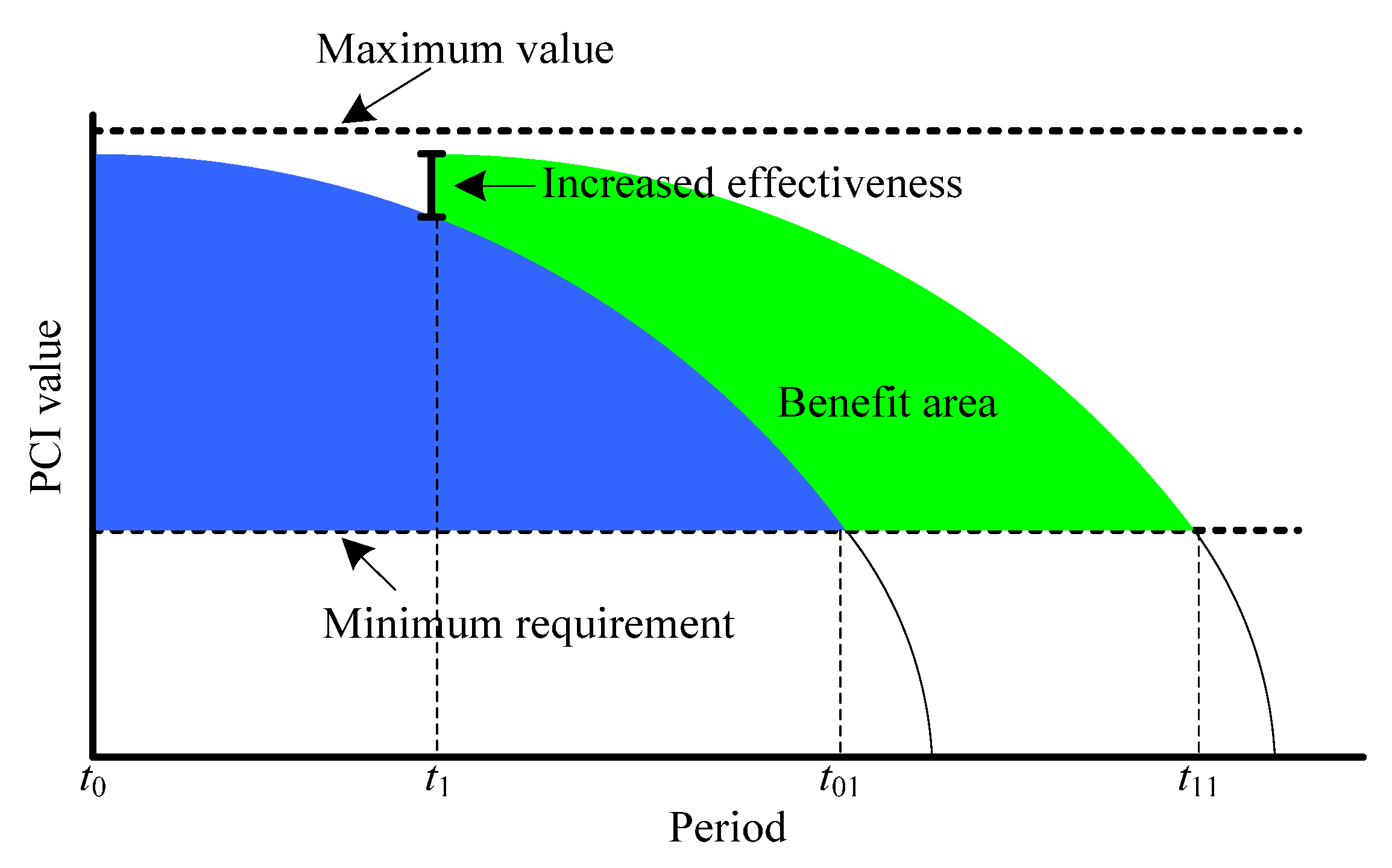
Maximize maintenance effectiveness: The primary goal of pavement maintenance is to provide better driving conditions for as many users as possible. This means that the decision should consider not only the immediate effects of maintenance (i.e., how is the pavement after maintenance?) but also the overall effectiveness (i.e., how many users can use roads in better condition?). Therefore, this paper uses the product of traffic flow and pavement condition as a decision objective to make maintenance decisions more scientific. Multiplying pavement condition by traffic flow considers that segments with higher traffic flow contribute more to overall effectiveness and, thus, are worth focusing on. This can be expressed as:

$$\max f_1={\displaystyle \sum _{m\in M}{\displaystyle \sum _{u\in U}{\displaystyle \sum _{i\in I}{s}_{i,u}\times V_{i,u,m}\times T_{u,m}}}}$$

(15)

(2)

Minimize carbon emissions: For pavement maintenance, while improving pavement conditions, there may be environmental impacts, including greenhouse gases, noise, dust, etc. Compared with low-altitude regions, the ecological environment in high-altitude regions is more fragile. Therefore, when formulating pavement maintenance plans for high-altitude regions, these adverse impacts should be given greater consideration. Hence, this paper sets minimizing carbon emissions as an optimization objective, which can be expressed as:

$$\min f_2={\displaystyle \sum _{j\in J}{\displaystyle \sum _{i\in I}{P}_j\times L_i\times B_i\times x_{i,j}}}$$

(16)

(3)

Minimize the affected traffic volume: During pavement maintenance, construction activities inevitably have adverse effects on traffic, especially when traffic flow is high. To reduce the interference of pavement maintenance on traffic, it is necessary to consider traffic management during construction and to schedule maintenance time reasonably. Based on this, this paper constructs an objective function to minimize the impact on traffic, combining the predicted monthly traffic volume, the working hours required for different maintenance methods, and the protection time required after maintenance, specifically expressed as:

$$\min f_3={\displaystyle \sum _{m\in M}{\displaystyle \sum _{u\in U}{\displaystyle \sum _{j\in J}{\displaystyle \sum _{i\in I}\left[\left(⌈\frac{G_j\times x_{i,j}\times L_i\times B_i}{Q\times O}⌉+D_j\times x_{i,j}\right)\times V_{i,u,m}\times y_{i,u,m}\right]}}}}$$

(17)

(4)

Minimizing the roughness index: The international roughness index (IRI) reflects the level of vibration and bumpiness experienced by vehicles traveling on the road [30,32], indicating that roughness affects the comfort of the driving experience. Additionally, roughness has a significant impact on energy consumption, with higher IRI values corresponding to higher energy consumption [32]. Therefore, to meet comfort needs and environmental protection requirements, minimizing IRI value as much as possible can be set as an optimization objective:

$$\min f_4={\displaystyle \sum _{u\in U}{\displaystyle \sum _{i\in I}{r}_{i,u}}}$$

(18)

(5)

Minimize maintenance costs: Minimizing maintenance costs as an optimization objective is a common approach in pavement maintenance decision [3]. The calculation of maintenance costs is related to the maintenance approach and maintenance area, and the corresponding objective function can be expressed as:

$$\min f_5={\displaystyle \sum _{j\in J}{\displaystyle \sum _{i\in I}{C}_j\times L_i\times B_i\times x_{i,j}}}$$

(19)

4. Model Transformation

It can be observed that the optimization model (the initial model, for short), composed of objective functions (15) to (19) and constraints (1) to (14), is a multi-objective nonlinear programming problem with both continuous variables ($s_{i,u}$ and $r_{i,u}$) and integer variables ($x_{i,j}$ and $y_{i,u,m}$), where it is difficult to obtain an exact solution via common methods. If we replace its nonlinear terms with linear terms, then it is transformed into a mixed-integer linear programming (MILP) problem. MILP problems are popular because of their mature solving techniques. Therefore, this paper further reconstructs it into a MILP problem by transforming the nonlinear terms.

4.1. Transformation of Nonlinear Terms

The presence of nonlinear terms increases the complexity of solving the model, and linearizing them aids in solving the model. Many scholars also often adopt exact algorithms or solvers to solve linear programming problems. For the initial model, five lemmas are proposed.

Lemma 1.

For Constraint (1), which is in the form of a piecewise function, it can be equivalently transformed by introducing an auxiliary variable  $v_{i,u}$ and a sufficiently large positive number  $\mathrm{M}$ as follows:

$$\left\{\begin{array}{l}{s}_{i,u}\le S_{i,0}\times e^{{\alpha }_{i,1}\times u+{\beta }_{i,1}}+{\displaystyle \sum _{m\in M}{\displaystyle \sum _{u*\in \{u*|u*\le u\}}{\displaystyle \sum _{j\in J}{x}_{i,j}\times E_j\times y_{i,u*,m}\times e^{{\alpha }_{i,1}\times (u-u*)+{\beta }_{i,1}}}}},\forall i\in I,u\in U\\ s_{i,u}\le S_{\max },\forall i\in I,u\in U\\ s_{i,u}\ge S_{\max }-\mathrm{M}\times (1-v_{i,u}),\forall i\in I,u\in U\\ s_{i,u}\ge S_{i,0}\times e^{{\alpha }_{i,1}\times u+{\beta }_{i,1}}+{\displaystyle \sum _{m\in M}{\displaystyle \sum _{u*\in \{u*|u*\le u\}}{\displaystyle \sum _{j\in J}{x}_{i,j}\times E_j\times y_{i,u*,m}\times e^{{\alpha }_{i,1}\times (u-u*)+{\beta }_{i,1}}}}}-\mathrm{M}\times v_{i,u},\forall i\in I,u\in U\\ v_{i,u}\in \{0,1\}\end{array}\right.$$

(20)

Lemma 2.

For Constraint (4), which includes logarithmic terms, both sides can be transformed into a linear form by taking their logarithms (i.e.,  $\ln (r_{i,u})=\ln ({\alpha }_{i,2})+{\beta }_{i,2}\times s_{i,u}$). Further, let  $r_{i,u}^{\prime }=\ln (r_{i,u})$, then we have:

$$r_{i,u}^{\prime }=\ln ({\alpha }_{i,2})+{\beta }_{i,2}\times s_{i,u}$$

(21)

Lemma 3.

For Objective function (18), combining Lemma 2 and the characteristics of the objective function, it can be transformed into the form of Equation (22).

$$\min f_4^{\prime }={\displaystyle \sum _{u\in U}{\displaystyle \sum _{i\in I}{r}_{i,u}^{\prime }}}$$

(22)

Lemma 4.

For the quadratic terms involving multiple decision variables (i.e.,$x_{i,j}\times y_{i,u,m}$), based on the properties of the decision variables, both types of variables are 0–1 variables. Therefore, as shown in

Table 3. Analysis of the value of $z_{i,j,u,m}$.

Case	${\mathit{x}}_{\mathit{i},\mathit{j}}$	${\mathit{y}}_{\mathit{i},\mathit{u},\mathit{m}}$	${\mathit{z}}_{\mathit{i},\mathit{j},\mathit{u},\mathit{m}}$
1	0	0	0
2	0	1	0
3	1	0	0
4	1	1	1

, if we let  $z_{i,j,u,m}=x_{i,j}\times y_{i,u,m}$, then the value of  $z_{i,j,u,m}$ can be determined accordingly.

Based on the contents in Table 3, the linear expression, $z_{i,j,u,m}=x_{i,j}\times y_{i,u,m}$, can be obtained as follows:

$$\left\{\begin{array}{l}{z}_{i,j,u,m}\le x_{i,j},\forall i\in I,j\in J,u\in U,m\in M\\ z_{i,j,u,m}\le y_{i,u,m},\forall i\in I,j\in J,u\in U,m\in M\\ z_{i,j,u,m}\ge x_{i,j}+y_{i,u,m}-1,\forall i\in I,j\in J,u\in U,m\in M\\ x_{i,j},y_{i,u,m},z_{i,j,u,m}\in \left\{0,1\right\},\forall i\in I,j\in J,u\in U,m\in M\end{array}\right.$$

(23)

Lemma 5.

For the model Objective function (17) and the integer signs involved in Constraint (7), the auxiliary variable  $h_{i,j}$  is introduced to replace  $⌈{\displaystyle \frac{G_j\times x_{i,j}\times L_i\times B_i}{Q\times O}}⌉$  within higher precision. In this case, the additional constraints are:

$$\left\{\begin{array}{l}{h}_{i,j}\ge {\displaystyle \frac{G_j\times x_{i,j}\times L_i\times B_i}{Q\times O}},\forall i\in I,j\in J\\ h_{i,j}\le {\displaystyle \frac{G_j\times x_{i,j}\times L_i\times B_i}{Q\times O}}+0.999,999,\forall i\in I,j\in J\end{array}\right.$$

(24)

Due to the introduction of  $h_{i,j}$, this paper introduces another situation of the product of decision variables. Based on the properties of the decision variables, $h_{i,j}$ is an integer variable in the range $\left[0,h_{\max }\right]$ ($h_{\max }$ is its maximum value), and $y_{i,u,m}$ is a 0–1 variable. Therefore, as shown in

Table 4. Analysis of the value of $n_{i,j,u,m}$.

Case	${\mathit{h}}_{\mathit{i},\mathit{j}}$	${\mathit{y}}_{\mathit{i},\mathit{u},\mathit{m}}$	${\mathit{n}}_{\mathit{i},\mathit{j},\mathit{u},\mathit{m}}$
1	$\left[0,h_{\max }\right]$	0	0
2	$\left[0,h_{\max }\right]$	1	$h_{i,j}$

, if we let $n_{i,j,u,m}=h_{i,j}\times y_{i,u,m}$, the value of the variable $n_{i,j,u,m}$ can be determined.

By organizing the value of $n_{i,j,u,m}$, the corresponding constraint can be obtained as follows:

$$\left\{\begin{array}{l}{n}_{i,j,u,m}\le h_{i,j},\forall i\in I,j\in J,u\in U,m\in M\\ n_{i,j,u,m}\ge h_{i,j}-h_{\max }\times \left(1-y_{i,u,m}\right),\forall i\in I,j\in J,u\in U,m\in M\\ n_{i,j,u,m}\le h_{\max }\times y_{i,u,m},\forall i\in I,j\in J,u\in U,m\in M\\ n_{i,j,u,m}\ge 0,\forall i\in I,j\in J,u\in U,m\in M\\ y_{i,u,m}\in \left\{0,1\right\},\forall i\in I,u\in U,m\in M\end{array}\right.$$

(25)

By incorporating the above transformation methods for nonlinear terms into the initial model, we obtain a multi-objective optimization model with linear characteristics, which belongs to a MILP problem (Equation (26)).

$$\begin{array}{l}\max f_1={\displaystyle \sum _{m\in M}{\displaystyle \sum _{u\in U}{\displaystyle \sum _{i\in I}{s}_{i,u}\times V_{i,u,m}\times T_{u,m}}}}\\ \min f_2={\displaystyle \sum _{j\in J}{\displaystyle \sum _{i\in I}{P}_j\times L_i\times B_i\times x_{i,j}}}\\ \min f_3^{\prime }={\displaystyle \sum _{m\in M}{\displaystyle \sum _{u\in U}{\displaystyle \sum _{j\in J}{\displaystyle \sum _{i\in I}(n_{i,j,u,m}\times V_{i,u,m}+D_j\times z_{i,j,u,m}\times V_{i,u,m})}}}}\\ \min f_4^{\prime }={\displaystyle \sum _{u\in U}{\displaystyle \sum _{i\in I}{r}_{i,u}^{\prime }}}\\ \min f_5={\displaystyle \sum _{j\in J}{\displaystyle \sum _{i\in I}{C}_j\times L_i\times B_i\times x_{i,j}}}\\ \begin{array}{l}s.t.\\ \\ \\ \\ \\ \\ \\ \\ \\ \\ \\ \\ \\ \\ \\ \\ \\ \\ \\ \\ \\ \\ \\ \\ \\ \\ \\ \\ \\ \\ \\ \\ \end{array}\{\begin{array}{l}{s}_{i,u}\le S_{i,0}\times e^{{\alpha }_{i,1}\times u+{\beta }_{i,1}}+{\displaystyle \sum _{m\in M}{\displaystyle \sum _{u*\in \{u*|u*\le u\}}{\displaystyle \sum _{j\in J}{z}_{i,j,u*,m}\times E_j\times e^{{\alpha }_{i,1}\times (u-u*)+{\beta }_{i,1}}}}},\forall i\in I,u\in U\\ s_{i,u}\ge S_{i,0}\times e^{{\alpha }_{i,1}\times u+{\beta }_{i,1}}+{\displaystyle \sum _{m\in M}{\displaystyle \sum _{u*\in \{u*|u*\le u\}}{\displaystyle \sum _{j\in J}{z}_{i,j,u*,m}\times E_j\times e^{{\alpha }_{i,1}\times (u-u*)+{\beta }_{i,1}}}}}-M\times v_{i,u},\forall i\in I,u\in U\\ s_{i,u}\ge S_{\max }-M\times (1-v_{i,u}),\forall i\in I,u\in U\\ s_{i,u}\le S_{\max },\forall i\in I,u\in U\\ r_{i,u}^{\prime }=\ln ({\alpha }_{i,2})+{\beta }_{i,2}\times s_{i,u},\forall i\in I,u\in U\\ {\displaystyle \sum _{j\in J}{\displaystyle \sum _{i\in I}{n}_{i,j,u,m}}}\le T_{u,m},\forall u\in U,m\in M\\ {\displaystyle \sum _{m\in M}{\displaystyle \sum _{u\in U}{\displaystyle \sum _{j\in J}{\displaystyle \sum _{i\in I}{C}_j\times L_i\times B_i\times z_{i,j,u,m}}}}}\le C_{\max }\\ {\displaystyle \sum _{m\in M}{\displaystyle \sum _{j\in J}{\displaystyle \sum _{i\in I}{C}_j\times L_i\times B_i\times z_{i,j,u,m}}}}\le C_{u,\max },\forall u\in U\\ h_{i,j}\ge {\displaystyle \frac{G_j\times x_{i,j}\times L_i\times B_i}{Q\times O}},\forall i\in I,j\in J\\ h_{i,j}\le {\displaystyle \frac{G_j\times x_{i,j}\times L_i\times B_i}{Q\times O}}+0.99999,\forall i\in I,j\in J\\ y_{i,u,m}\ge 0,\forall i\in I,u\in U,m\in M_s\\ y_{i,u,m}=0,\forall i\in I,u\in U,m\in M_u\\ z_{i,j,u,m}\ge x_{i,j}+y_{i,u,m}-1,\forall i\in I,j\in J,u\in U,m\in M\\ z_{i,j,u,m}\le x_{i,j},\forall i\in I,j\in J,u\in U,m\in M\\ z_{i,j,u,m}\le y_{i,u,m},\forall i\in I,j\in J,u\in U,m\in M\\ n_{i,j,u,m}\le h_{i,j},\forall i\in I,j\in J,u\in U,m\in M\\ n_{i,j,u,m}\ge h_{i,j}-h_{\max }\times \left(1-y_{i,u,m}\right),\forall i\in I,j\in J,u\in U,m\in M\\ n_{i,j,u,m}\le h_{\max }\times y_{i,u,m},\forall i\in I,j\in J,u\in U,m\in M\\ n_{i,j,u,m}\ge 0,\forall i\in I,j\in J,u\in U,m\in M\\ \mathrm{Constraints}(2),(3),(5),(6),(10)-(12)\\ x_{i,j}\in \left\{0,1\right\},\forall i\in I,j\in J\\ v_{i,u}\in \left\{0,1\right\},\forall i\in I,u\in U\\ y_{i,u,m}\in \left\{0,1\right\},\forall i\in I,u\in U,m\in M\\ z_{i,j,u,m}\in \left\{0,1\right\},\forall i\in I,j\in J,u\in U,m\in M\end{array}\end{array}$$

(26)

4.2. Transformation of Multi-Objective Functions

Multi-objective optimization problems (MOPs) involve trade-offs between multiple decision objectives. A common approach is to transform an MOP problem into a single-objective optimization problem, thereby using more conventional single-objective optimization solution methods.

Specifically, we first refer to Ref. [13] to unify the magnitudes of each sub-objective, eliminating the impact of magnitude differences on results. Furthermore, we use the weighted sum method to integrate different decision objectives into one objective function, achieving the transformation from an MOP to a single-objective optimization problem, as shown in Equation (27).

$$\min F=w_1\times {\displaystyle \frac{-f_1}{f_{1,\max }}}+w_2\times {\displaystyle \frac{f_2}{f_{2,\min }}}+w_3\times {\displaystyle \frac{{f_3}^{\prime }}{{{f_3}^{\prime }}_{,\min }}}+w_4\times {\displaystyle \frac{f_4^{\prime }}{{{f_4}^{\prime }}_{,\min }}}+w_5\times {\displaystyle \frac{f_5}{f_{5,\min }}}$$

(27)

In summary, by combining Equations (26) and (27), the transformed mathematical model belongs to the typical MILP problem with one objective function. This type of problem has a wealth of solution methods, including common solvers (e.g., Cplex, Lingo, or Gurobi), making it more applicable compared with the initial model.

Additionally, considering the preferences of different decision-makers, we further focused on the tendencies of different objective functions and proposed five types of decision strategies, as shown in

Table 5. Weight ranges for sub-objectives corresponding to different decision strategies.

Strategy	Objective	Weight Ranges
		${\mathit{w}}_1$	${\mathit{w}}_2$	${\mathit{w}}_3$	${\mathit{w}}_4$	${\mathit{w}}_5$
1	Optimize maintenance effectiveness	>0	=0	=0	>0	=0
2	Optimize cost savings	=0	=0	=0	=0	>0
3	Optimize affected traffic volume	=0	=0	>0	=0	=0
4	Optimize environmental protection	=0	>0	=0	=0	=0
5	Balance all the above considerations	>0	>0	>0	>0	>0

. Obviously, the maintenance plans derived from different decision strategies are not the same, and the differences among them are discussed in Section 5.

5. Case Analysis

5.1. Case Description

To analyze the effectiveness of the pavement maintenance decision model, this paper conducted a simulation analysis using pavement maintenance data from high-altitude regions obtained through surveys. Specifically, codes were written in Python language, and the Gurobi solver was utilized to solve the optimization models, with the termination condition set to a 0.1% gap between the upper and lower bounds. The hardware used was a laptop equipped with a Win 10 system, an Intel(R) Core (TM) i7-10750H CPU (Interl, Santa Clara, CA, USA), and 32 GB of memory.

In the simulation analysis, we focused on 30 road segments, starting from their state at the end of 2023 and aiming at developing a maintenance plan for the next three years. Each year includes 12 months, with April to October being suitable for maintenance and November to March being unsuitable. Each road segment has the corresponding predicted traffic flow data and an initial PCI value, with initial PCI values ranging from 63 to 86. The annual average daily traffic (AADT) and monthly traffic volume for each road segment were recorded. Specifically, the basic information of the 30 road segments is shown in

Table 6. Statistics of basic information of road segments.

Segment	Length/m	Width/m	AADT	Initial PCI	Segment	Length/m	Width/m	AADT	Initial PCI
01	180	4.5	6000	78	16	810	3.5	3560	81
02	190	3.5	5200	80	17	220	3	12,400	82
03	400	4	7200	79	18	320	3.5	9200	75
04	260	3.5	5200	78	19	100	3	12,000	76
05	300	4	8800	81	20	80	4	9600	82
06	320	3	7200	78	21	920	3.5	7600	75
07	280	3	7200	81	22	610	3	6800	77
08	90	3.5	6400	76	23	230	3.5	6000	81
09	70	3	5600	81	24	340	4	5600	76
10	288	3	8400	78	25	550	4.5	8400	80
11	165	4.5	10,000	75	26	290	3	3840	78
12	180	3.5	6800	80	27	280	3.5	9200	80
13	580	3	8000	82	28	650	3.5	6800	77
14	620	3	7200	76	29	280	3	5200	79
15	750	4	6400	79	30	660	3	4400	81

, and the predicted monthly traffic volume of each segment in 2024 is shown in Figure 2.

Regarding the maintenance approaches, we classified them into five categories and statistically analyzed their related attributes based on survey data, as shown in

Table 7. Characteristics of different maintenance methods.

Approach	Working Hours (hours/m²)	Carbon Emissions (kg/m²)	Protection Days	Cost (CNY/m²)	Effectiveness
1	0.2	8	1	10	3
2	0.5	15	2	25	5
3	0.75	32	2	100	20
4	1	50	3	200	30
5	1.5	80	3	400	45

. The five maintenance approaches are filling cracks, patching potholes, chip seal coating or using a slurry seal, resurfacing with partial reconstruction, and complete reconstruction [1]. These approaches cover different levels from minor repairs to major maintenance. When adopting different maintenance approaches, the required working hours, protection days, and costs per unit area vary, and these model parameters are set based on the survey data. For carbon emissions, considering the impact of altitude, the settings are based on Refs. [29,30].

For other parameters, the annual budget was set to CNY 600,000, with a total budget of CNY 1,500,000. The number of available workers was 20, and the daily working hours were 8 h. Meanwhile, the average PCI value requirement for the segments was set to 76, with a minimum value of 72 and a maximum value of 100. The parameters ${\alpha }_{i,1}$ and ${\beta }_{i,1}$ for Constraint (1) were set to −0.05 and −0.02, respectively. The parameters ${\alpha }_{i,2}$ and ${\beta }_{i,2}$ for Constraint (4) were set to 16.074 and −0.026, respectively. Additionally, the sufficiently large positive number $\mathrm{M}$ was set to 200.

Regarding the objective functions, the five sub-objectives mentioned above were individually set as the model’s decision objectives. The solutions for the five models were obtained with the above parameters. The maximum value for Objective function (14) is 19,418,050,875.175, the minimum value for Objective function (15) is 650,053, the minimum value for Objective function (16) is 856,268, the minimum value for Objective function (17) is 59.186, and the minimum value for Objective function (18) is 1,383,646. Based on this, the differences in magnitude among them can be eliminated using Equation (26). For the five decision strategies, we set the corresponding weights according to

Table 8. Sub-objective weights for different decision strategies.

Strategy	Objective	Weights
		${\mathit{w}}_1$	${\mathit{w}}_2$	${\mathit{w}}_3$	${\mathit{w}}_4$	${\mathit{w}}_5$
1	Optimize maintenance effectiveness	0.5	0	0	0.5	0
2	Optimize cost savings	0	0	0	0	1
3	Optimize affected traffic volume	0	0	1	0	0
4	Optimize environmental protection	0	1	0	0	0
5	Balance all the above considerations	0.2	0.2	0.2	0.2	0.2
Baseline	Optimize effectiveness and minimize cost	0.5	0	0	0	0.5

. In the simulation analysis, these five decision strategies were all discussed. Furthermore, to analyze the model’s effectiveness, a baseline strategy was considered. This baseline strategy, commonly adopted in previous studies, aims for optimal effectiveness and minimal cost. It should be noted that, unlike other models, the baseline strategy’s maintenance decision model assumes that maintenance can occur in any month of the year, which was the default assumption in previous research.

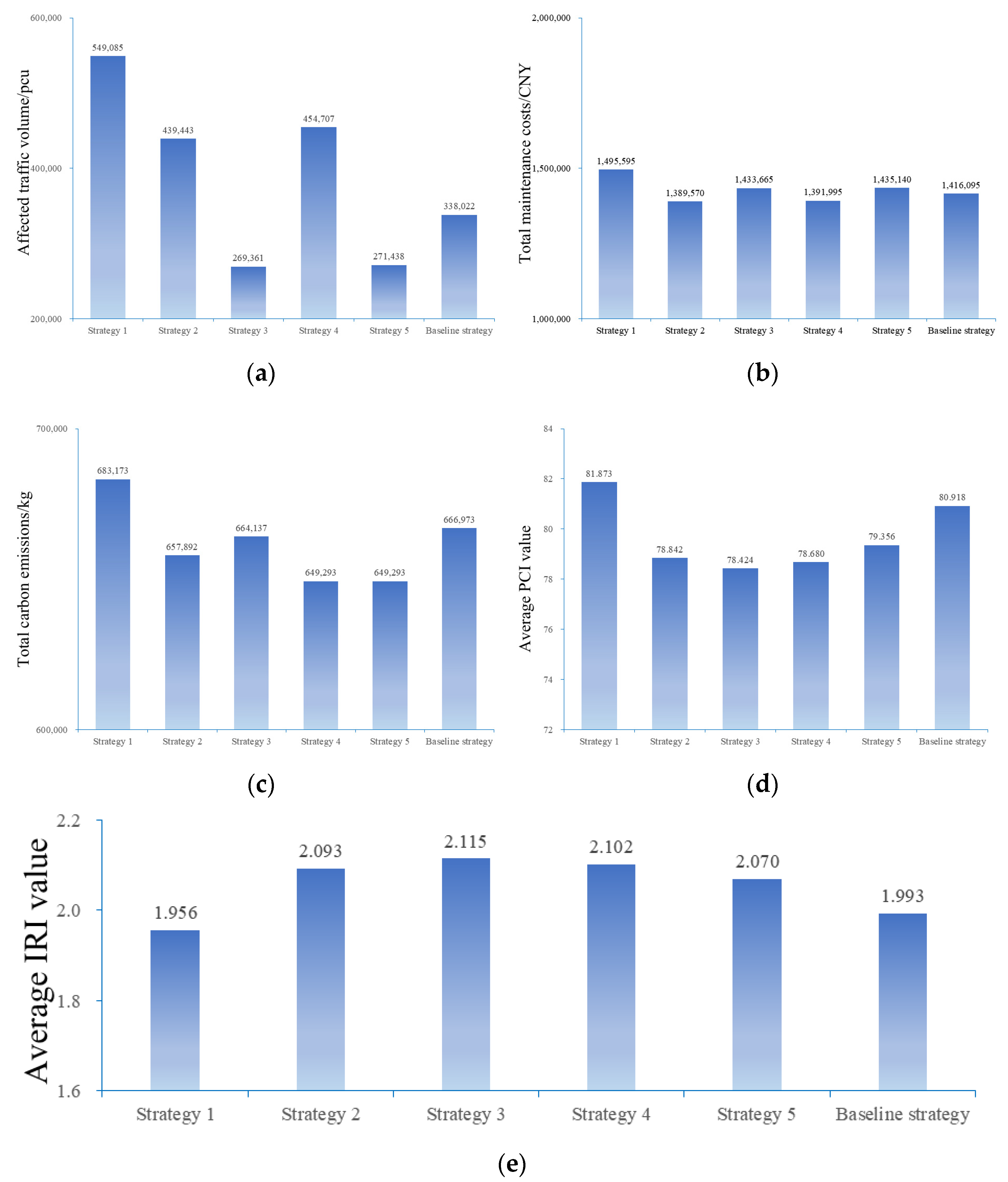
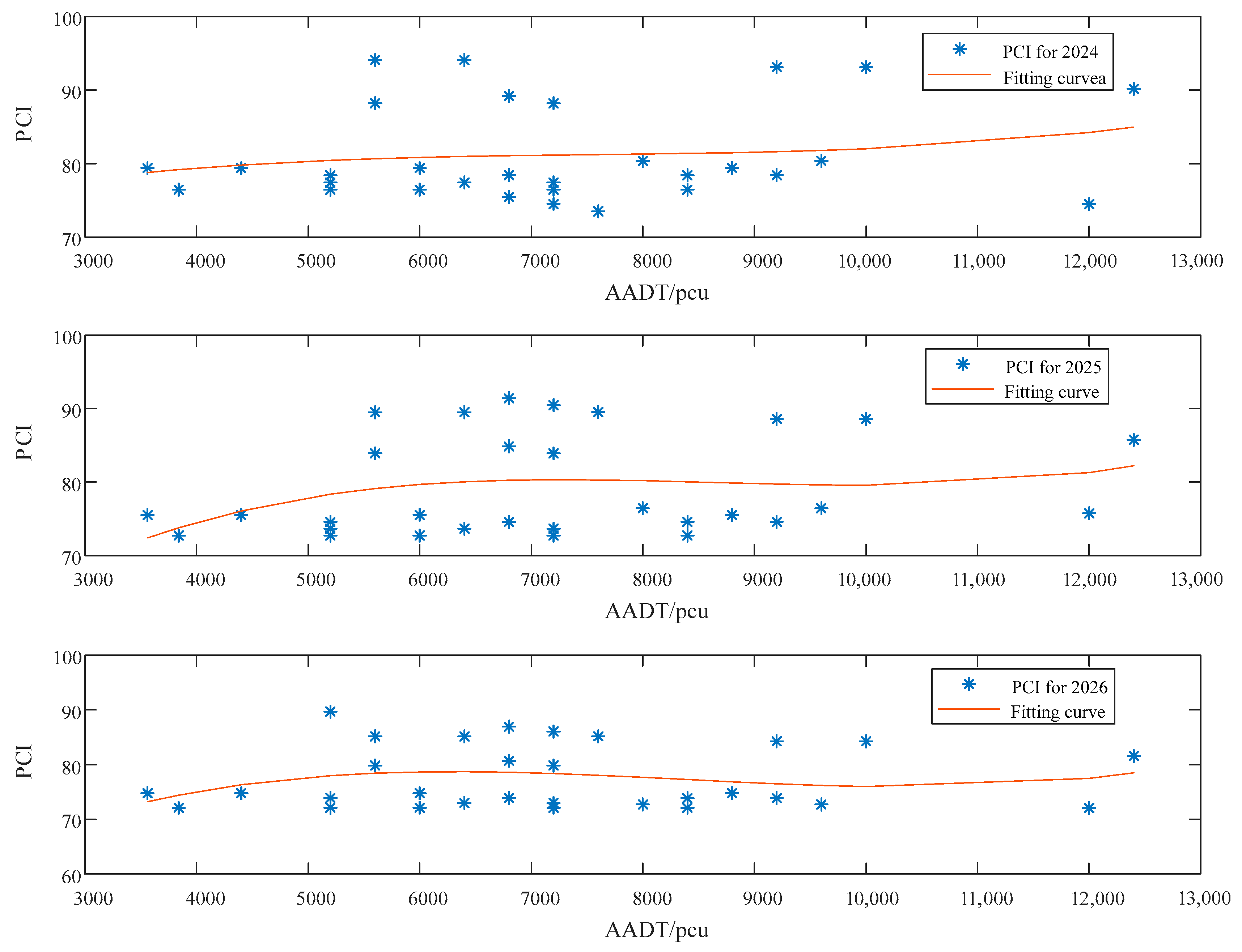
5.2. Result Analysis

Simulation calculations show that the models with different decision strategies can all be solved within seconds. Specifically, the solution time for the model with Strategy 1 is 5.19 s, Strategy 2 is 9.89 s, Strategy 3 is 7.36 s, Strategy 4 is 8.34 s, and Strategy 5 is 6.72 s. Moreover, the obtained decision plans satisfy the set constraints, indicating that the constructed models are effective and highly applicable.

Regarding the model solution results, the indexes including affected traffic volume, total maintenance costs, total carbon emissions, average PCI value, and average IRI value are discussed based on the five strategies. First, Figure 3a shows the affected traffic volume under different strategies. It can be seen that the affected traffic volume for Strategy 1 is the highest, followed by Strategies 2 and 3, while Strategies 3 and 5 have the lowest values. This is because Strategy 1 focuses more on maintenance effectiveness, tending to choose plans that significantly improve the PCI value, which also requires more working hours. Additionally, ignoring the distribution of traffic flow may also be a factor contributing to a higher affected traffic volume under this strategy. For Strategies 2 and 3, despite their tendency toward lower cost or lower carbon emission plans, as shown in Table 7, ignoring the distribution of traffic flow results in higher affected traffic volumes. For Strategies 3 and 5, both of which involve minimizing the affected traffic volume as a decision objective, the values are smaller and very close.

Figure 3b shows the maintenance costs under different decision strategies. It can be seen that the maintenance costs for Strategy 1 are the highest, followed by Strategies 3 and 5, with Strategies 2 and 4 being the lowest. This is because the objective function of Strategy 1 tends to favor solutions that significantly improve the PCI value, but these solutions also require higher costs. For Strategy 3, it focuses more on the impact of the maintenance plan on traffic flow. As for Strategy 5, although it considers maintenance costs, it also takes other decision objectives into account, so neither fully prioritizes minimizing costs. For Strategy 2, which aims solely to minimize costs, the cost-saving effect is the most ideal. Additionally, since maintenance approaches with lower costs also result in lower carbon emissions (see Table 7), the results of Strategy 4 are very close to those of Strategy 2.

Figure 3c further presents the carbon emissions of maintenance plans under different strategies. It can be seen that the carbon emissions for Strategy 1 are the highest, followed by Strategies 3 and 5, with Strategies 2 and 4 being the lowest. This result closely aligns with the conclusions in Figure 3b, primarily because maintenance plans with lower carbon emissions also tend to have relatively lower costs (see Table 7). Strategy 4 aims solely to minimize carbon emissions, thus resulting in the most ideal carbon emission values.

Figure 3d,e shows the average PCI values and average IRI values under different strategies. A higher PCI value indicates a better pavement condition, while a lower IRI value also indicates a better pavement condition. From the two figures, it can be seen that the values corresponding to Strategy 1 are the most ideal, which is related to the strategy’s primary focus on maintenance effectiveness. Meanwhile, the values corresponding to Strategies 2, 3, and 4 are relatively less ideal because their solutions tend to favor maintenance approaches that require lower costs and result in lower carbon emissions or shorter working hours. However, such maintenance approaches have a relatively smaller improvement effect on pavement conditions. As for Strategy 5, which considers maintenance effectiveness, the resulting values are relatively more ideal compared with Strategies 2, 3, and 4.

Based on the above analysis, it can be observed that some decision objectives are interrelated, such as Strategy 4 focusing on minimizing carbon emissions and Strategy 2 focusing on minimizing maintenance costs. More importantly, Strategy 5 considers all objective functions simultaneously and achieves acceptable results across different indicators. This can be seen in Figure 3a–e where the corresponding values are all between the respective maximum and minimum values. Therefore, if multiple decision needs are considered simultaneously, Strategy 5 is an optional approach. Based on the results, compared with the Baseline strategy, Strategy 5 resulted in 19.698% less affected traffic volume, 2.651% less carbon emissions, 1.344% more maintenance costs, 1.260% less average PCI, and 3.864% more average IRI. Further analysis of

Table 9. Maintenance plans based on the Baseline strategy and Strategy 5.

Segment	Baseline Strategy			Strategy 5			PCI Values Based on Strategy 5
	Approach	Year	Month	Approach	Year	Month	2024	2025	2026
1	1	3	1	1	3	10	76.455	72.727	72.120
2	1	1	5	1	3	10	78.416	74.592	73.894
3	1	2	12	1	3	10	77.436	73.659	73.007
4	1	3	3	1	3	10	76.455	72.727	72.120
5	1	3	6	1	3	10	79.396	75.524	74.781
6	1	3	9	1	3	10	76.455	72.727	72.120
7	3	1	1	3	1	10	88.218	83.915	79.823
8	3	1	3	3	1	10	94.099	89.510	85.144
9	3	1	7	3	1	10	88.218	83.915	79.823
10	3	1	6	1	3	10	76.455	72.727	72.120
11	3	1	3	3	1	10	93.119	88.577	84.257
12	1	1	1	1	3	10	78.416	74.592	73.894
13	1	3	11	None	None	None	80.376	76.456	72.727
14	3	2	2	3	2	6	74.495	90.466	86.054
15	1	3	11	1	3	10	77.436	73.659	73.007
16	1	3	9	1	3	6	79.396	75.524	74.781
17	3	1	1	3	1	10	90.178	85.780	81.597
18	3	1	11	3	1	10	93.119	88.577	84.257
19	3	1	4	2	2	10	74.495	75.763	72.068
20	3	1	2	None	None	None	80.376	76.456	72.727
21	3	2	1	3	2	10	73.515	89.534	85.167
22	3	1	2	3	1	10	89.198	84.848	80.710
23	1	2	9	1	3	10	79.396	75.524	74.781
24	2	2	11	3	1	6	94.099	89.510	85.144
25	1	3	4	1	3	10	78.416	74.592	73.894
26	3	3	4	1	3	6	76.455	72.727	72.120
27	1	1	12	1	3	10	78.416	74.592	73.894
28	2	2	2	3	2	10	75.475	91.398	86.941
29	3	2	6	3	3	10	77.436	73.659	89.671
30	1	3	10	1	3	6	79.396	75.524	74.781

reveals that the Baseline strategy did not account for the impact of seasonal factors on the difficulty or suitability for maintenance, resulting in some maintenance tasks being scheduled during unsuitable months (e.g., Segments 1, 7, 12) and some segments being maintained during high-traffic months (e.g., Segment 5). Additionally, Table 9 shows that due to cost factors considered in the decision strategy, some segments with a good initial condition were allocated as “no maintenance task”, while segments needing maintenance were assigned different maintenance approaches and scheduled in months with lower traffic volumes in different years, and these months were suitable for maintenance tasks. In summary, the model presented in this paper, especially the maintenance decision model based on Strategy 5, is more suitable for high-altitude regions.

Combining Table 9 and the annual average daily traffic (AADT) of different segments, Figure 4 shows the correlation between traffic flow and PCI values, with a cubic fitting curve drawn. It can be seen that in the first year (2024), the curve is increasing, and the increasing trend is less pronounced in the second and third years, but still observable. This increasing trend indicates that segments with higher traffic flow tend to have higher PCI values. This result is related to the objective function “maximize maintenance effectiveness” included in Strategy 5, which aims for better pavement conditions on segments with higher traffic flow.

Additionally, we conducted sensitivity analyses based on Strategy 5, including the impact of the number of workers on affected traffic volume (see Figure 5a), the impact of the minimum requirement of PCI on carbon emissions during maintenance (see Figure 5b), and the impact of the annual budget on average PCI (see Figure 5c).

Figure 5a shows that the more maintenance workers, the less the traffic volume is affected under the same decision strategy. This result is relatively easy to understand: For the same maintenance task, the more workers, the shorter the required maintenance time or period, and the less the traffic flow is affected. Therefore, to minimize the impact of pavement maintenance on traffic, it is necessary to employ an appropriate number of workers.

Figure 5b shows that the higher the minimum requirement of PCI for the pavement, the more carbon emissions are generated during maintenance. This result is also easy to understand: For the same set of road segments, the higher the PCI required, the more significant the required maintenance effect (see Figure 1 and Table 7) and the higher the corresponding carbon emissions. Based on this, for maintenance planning, appropriately lowering the minimum requirement of PCI can help reduce carbon emissions.

Figure 5c shows the impact of the annual budget on the average PCI. It can be seen that the annual budget imposes certain constraints on the average PCI. This result is also easy to understand as a larger budget allows for more maintenance tasks and a wider selection of maintenance approaches to be implemented. Therefore, to ensure the quality of pavement maintenance, it is necessary to provide a maintenance budget matching the tasks.

6. Extension of the Maintenance Decision Model

6.1. Interval Number

In actual maintenance, due to market price fluctuations, the unit area maintenance cost ($C_j$) has uncertainty. Uncertain parameters can be described using fuzzy numbers, ambiguous numbers, and interval numbers. Since the range of uncertain numbers is generally determinable, this paper uses interval numbers [33] for description. Specifically, for maintenance cost $C_j$, its uncertain form is $\widetilde{C_j}$. If $-\infty <\underset{¯}{C_j}\le \overline{C_j}<+\infty$, then $\widetilde{C_j}$= [$\underset{¯}{C_j},\overline{C_j}$] is an interval number. If $\widetilde{C_j}=\underset{¯}{C_j}=\overline{C_j}$, then $\widetilde{C_j}$ degenerates into a real number, which is a deterministic value.

6.2. Optimistic Solution and Pessimistic Solution

For optimization models, when the feasible region of decision variables is the largest and the best objective function is used, the best optimal solution can be obtained, which is the optimistic solution, and the corresponding model is called the optimistic sub-model. Conversely, when the feasible region is the smallest and the worst objective function is used, the worst optimal solution can be obtained, which is the pessimistic solution, and the corresponding model is called the pessimistic sub-model [34]. For the maintenance decision model in this paper, considering uncertainty, the objective function value corresponding to the optimistic model represents the minimum value under the optimistic condition where the uncertain parameter $\widetilde{C_j}$ takes the lower limit. Similarly, the objective function value corresponding to the pessimistic model represents the minimum value under the pessimistic condition where the uncertain parameter takes the upper limit.

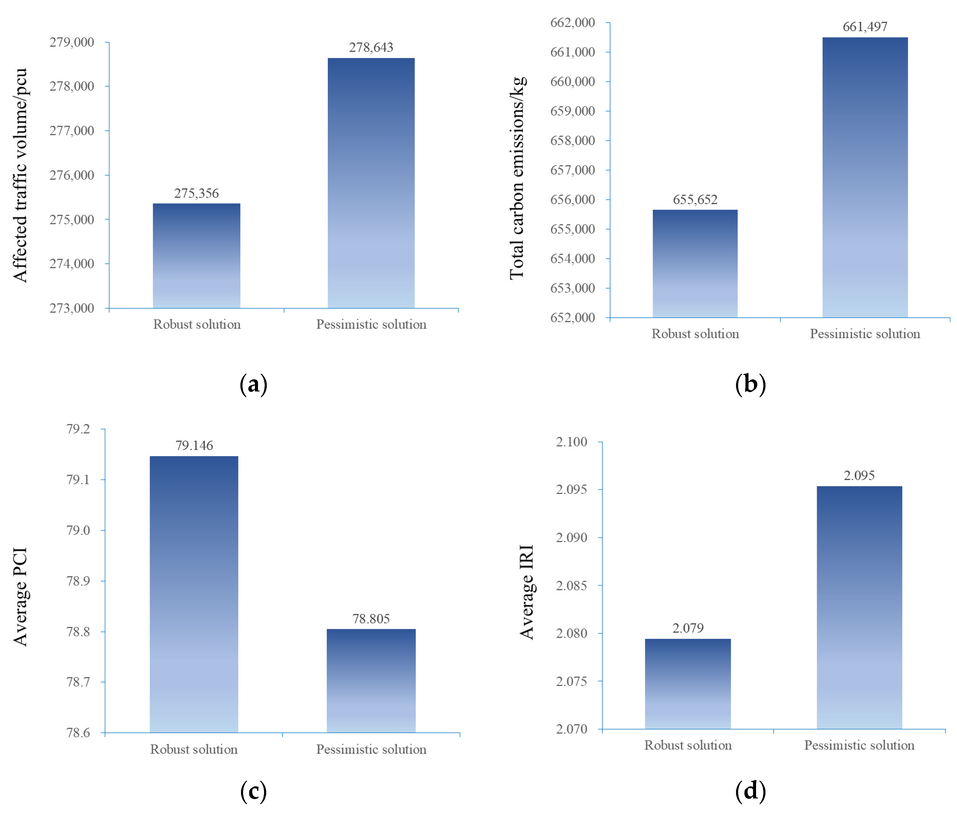
6.3. Robust Solution and Analysis

Obtaining a solution that is minimally affected by uncertainties is the focus of robust optimization. The pessimistic solution obtained under the pessimistic condition is definitely a robust solution, but the corresponding result is likely to be overly conservative. In response to this, Li et al. [34] proposed a robust optimization method based on the acceptable objective variation range (AOVR). This method requires the decision variables to be independent of the uncertain parameters and aims to find a robust solution such that, under the maximum fluctuation caused by the uncertain parameters, the fluctuation range of the objective function value does not exceed the acceptable range. Based on this, a robust optimization model as shown in Equation (28) is further proposed.

$$\begin{array}{l}\min F^{\prime }=A_{*}^{\mathrm{T}}X+c_{*}\\ \begin{array}{c}\begin{array}{l}s.t.\\ \\ \\ \\ \end{array}\left\{\begin{array}{l}{\displaystyle \sum _{j\in J}{\displaystyle \sum _{i\in I}{(x_{i,j}-x_{i,j,*})}^2\le \epsilon }}\\ {\tilde{e}}_p^{\mathrm{T}}X\le {\tilde{h}}_p,\forall p\in \{1,2,\cdots ,N_c\}\\ X\in \{0,1\}\end{array}\right.\end{array}\end{array}$$

(28)

where $A_{*}$ and $c_{*}$, respectively, represent the coefficient vector and constant term vector formed by the nominal values of each uncertain parameter in the optimistic model. $X$ represents the decision variable vector. ${\tilde{e}}_p$ and ${\tilde{h}}_p$ represent the coefficient vector and constant term of the constraint equation, respectively, taking the parameters corresponding to the pessimistic model. $N_c$ represents the number of constraints. $x_{i,j,*}$ represents the value of $x_{i,j}$ in the optimistic model solution. $\epsilon$ is the acceptable variation range, which limits the fluctuation range of the solution and the objective function value. This range should be as small as possible (but too small may result in no feasible solution) to obtain a robust solution as close as possible to the optimistic solution.

Since $x_{i,j}$ is a binary variable, the robust optimization model shown in Equation (28) also belongs to the MILP problem, which can be directly solved using the Gurobi solver. For this, based on the parameters in Section 5.1 and Strategy 5, we set $\widetilde{C_j}$= [$0.95\times C_j,1.05\times C_j$] (i.e., the cost variation coefficient is between 0.95 and 1.05), and set $\epsilon$ to 50 to obtain a robust solution.

Table 10. Results of the optimistic solution.

Segment	Approach	Segment	Approach	Segment	Approach
1	1	11	3	21	3
2	1	12	1	22	3
3	1	13	none	23	1
4	1	14	3	24	3
5	1	15	1	25	1
6	1	16	1	26	1
7	3	17	3	27	1
8	3	18	3	28	3
9	3	19	2	29	3
10	1	20	none	30	1

displays the optimization results for the optimistic solution. Figure 6 shows some results corresponding to the pessimistic solution and the robust solution.

At this point, the total cost is CNY 1,363,383, which is below the CNY 1,500,000 threshold. The annual costs are CNY 594,700, CNY 567,340, and CNY 201,343, all of which are under CNY 600,000, meeting the relevant constraints.

However, when the unit area maintenance cost is in the worst-case condition ($1.05\times C_j$), the total cost increases to CNY 1,506,897, exceeding the limit (CNY 1,500,000). The annual costs are CNY 657,300, CNY 627,060, and CNY 222,537, with the first two years exceeding CNY 600,000, thereby failing to meet the relevant constraints. Consequently, the optimistic solution becomes infeasible. This indicates that as the unit area maintenance cost gradually increases, the optimistic solution may transition from feasible to infeasible.

The results shown in Figure 6 indicate that for the four indicators involved—affected traffic volume, carbon emissions, evaluated PCI, and average IRI—the maintenance plan corresponding to the robust solution is more ideal compared with the plan corresponding to the pessimistic solution, showing advantages of 1.180%, 0.884%, 0.433%, and 0.767%, respectively. This is because the obtained robust solution has a high degree of proximity to the optimistic solution, and the feasible region corresponding to the optimistic sub-model is the largest, allowing for the best optimum solution. In contrast, for the pessimistic sub-model, the feasible region is the smallest, and the obtained optimum solution is the worst optimum solution [33,34]. Therefore, the robust model can provide a balanced maintenance plan.

The results shown in Figure 7 indicate that as the unit maintenance cost gradually increases, the total maintenance cost corresponding to the robust solution is always less than the cost corresponding to the pessimistic solution. This demonstrates that the robust solution obtained through the robust optimization model is superior to the pessimistic solution in dealing with variable maintenance costs, thereby further proving the effectiveness of robust optimization.

7. Conclusions

This paper proposes a pavement maintenance optimization decision method for high-altitude areas. The goal is to obtain a monthly maintenance plan by incorporating the impact of high-altitude climates on pavement maintenance, the effects of pavement maintenance on traffic and the ecological environment, and maintenance cost factors into the optimization decision requirements. It also addresses the influence of decision preferences on related indicators of pavement maintenance plans and constructs mixed-integer linear programming (MILP) models from the perspectives of common optimization and robust optimization. The conclusions drawn from the case analysis are summarized as follows:

Incorporating multiple decision objectives into the optimization model provides an acceptable compromise compared with considering only a single decision objective. When single or similar decision objectives are considered (e.g., Strategies 1 to 4), the optimal solutions tend to favor their corresponding decision objectives. For instance, if the goal is solely to optimize pavement maintenance effectiveness (i.e., Strategy 1), the affected traffic volume is the largest. When multiple decision objectives with conflicting relationships are considered, the multi-objective optimization method can obtain a balanced solution. For example, the maintenance plan derived from Strategy 5, which comprehensively considers various decision objectives, results in indicators that are all less than the corresponding maximum values and greater than the corresponding minimum values.

Compared with previous models, incorporating the unique needs of high-altitude pavement maintenance into the optimization model and refining the maintenance timing can yield more feasible decision plans. For example, decision models that only consider carbon emissions and costs may result in less feasible outcomes. Maintenance timing might be scheduled in months unsuitable for construction or during high-traffic periods.

Equipping with suitable pavement maintenance decision premises can lead to better comprehensive maintenance effects. For instance, when the number of maintenance workers increases from 15 to 20, the affected traffic volume decreases from 276,218 pcu to 265,147 pcu, a reduction of 4%. This indicates that reasonably increasing the number of workers can effectively mitigate the impact of maintenance tasks on traffic.

Robust optimization is one effective method to address uncertainties in pavement maintenance decisions. By targeting the uncertainty of unit area maintenance costs and employing a robust optimization method based on the acceptable objective variation range (AOVR), it is possible to derive a maintenance plan that considers the worst-case conditions (i.e., the least favorable unit maintenance cost) yet remains relatively positive. For example, in the case study, the optimistic solution becomes infeasible as unit area maintenance costs increase, and the robust solution outperforms the pessimistic solution in terms of affected traffic volume, carbon emissions, average PCI, and average IRI.

In future research, the scope of parameters can be expanded to cover more different types of roads and environmental conditions in high-altitude areas, thereby enhancing the model’s precision and applicability. Additionally, more comprehensive decision variables and constraints can be introduced into the model, such as considering dynamic changes in traffic demand and scheduling multiple maintenance activities. Moreover, attention can also be given to other environmental indicators beyond carbon emissions to more comprehensively assess the environmental impact of pavement maintenance. Additionally, considering the potential of nonlinear programming methods in handling similar problems, accurate and efficient nonlinear solutions are also worth exploring.

References

1. He, Z.; Sun, X. Discrete optimization models and methods for management systems of pavement maintenance and rehabilitation. J. Shanghai Univ. 2010, 14, 217–222. [Google Scholar] [CrossRef]
2. Ling, J.; Wang, Z.; Liu, S.; Tian, Y. Preventive Maintenance Decision-Making Optimization Method for Airport Runway Composite Pavements. Appl. Sci. 2024, 14, 3850. [Google Scholar] [CrossRef]
3. Pourgholamali, M.; Labi, S.; Sinha, K.C. Multi-objective optimization in highway pavement maintenance and rehabilitation project selection and scheduling: A state-of-the-art review. J. Road Eng. 2023, 3, 239–251. [Google Scholar] [CrossRef]
4. Wu, Q.; Li, C.; Xu, P. Comparative Study on the Laboratory and Field Aging Behavior of Asphalt Binders in High-altitude Regions. Technol. Highw. Transp. 2024, 40, 73–81. [Google Scholar]
5. Dou, M.; Hu, C.; Duoji, L.; He, Z. Analysis on Surface Troubles of the Qinghai-Tibet Highway. J. Glaciol. Geocryol. 2003, 25, 439–444. [Google Scholar]
6. Xu, P.; Zhu, X.; Yao, D.; Shi, C.; Qian, G. Review on intelligent detection and decision of asphalt pavement maintenance. J. Cent. South Univ. (Sci. Technol.) 2021, 52, 2099–2117. [Google Scholar]
7. Zhang, X. Research on Intelligent Maintenance Decision Method for the Whole Life Cycle of Road Network Infrastructure. Doctoral Dissertation, Southeast University, Nanjing, China, 2022. (In Chinese). [Google Scholar]
8. Yu, B.; Gu, X.; Ni, F.; Guo, R. Multi-objective optimization for asphalt pavement maintenance plans at project level: Integrating performance, cost and environment. Transp. Res. Part D 2015, 41, 64–74. [Google Scholar] [CrossRef]
9. Wang, C.H.; Wang, L.J.; Bai, J.H.; Liu, Y.D.; Wang, X.C. Research on Integration Optimization of Asphalt Pavement Preventive Maintenance Timing and Countermeasures During Period. China J. Highw. Transp. 2010, 23, 27–34. [Google Scholar]
10. Li, L.; Guan, T. Decision method for preventive maintenance of asphalt pavements considering multiple damage characteristics. J. Shanghai Univ. (Nat. Sci. Ed.) 2022, 28, 689–701. [Google Scholar]
11. Zhang, Y.; Shen, A.; Hou, Y. Application of Fund-target Optimization Method in Pavement Maintenance Decision. J. Highw. Transp. Res. Dev. 2018, 35, 34–40. [Google Scholar]
12. Mahmood, M.; Mathavan, S.; Rahman, M. A Parameter-free Discrete Particle Swarm Algorithm and Its Application to Multi-objective Pavement Maintenance Schemes. Swarm Evol. Comput. 2018, 43, 69–87. [Google Scholar] [CrossRef]
13. Sun, Y.; Hu, M.; Zhou, W.; Xu, W. Multiobjective optimization for pavement network maintenance and rehabilitation programming: A case study in Shanghai, China. Math. Probl. Eng. 2020, 2020, 3109156. [Google Scholar] [CrossRef]
14. Chen, Z.; Wang, D. Numerical analysis of a multi-objective maintenance decision model for sustainable highway networks: Integrating the GDE3 method, LCA and LCCA. Energy Build. 2023, 290, 113096. [Google Scholar] [CrossRef]
15. Lee, J.; Madanat, S. Optimal policies for greenhouse gas emission minimization under multiple agency budget constraints in pavement management. Transp. Res. Part D 2017, 55, 39–50. [Google Scholar] [CrossRef]
16. Elhadidy, A.A.; Elbeltagi, E.E.; Ammar, M.A. Optimum analysis of pavement maintenance using multi-objective genetic algorithms. HBRC J. 2015, 11, 107–113. [Google Scholar] [CrossRef]
17. Fani, A.; Golroo, A.; Mirhassani, S.A.; Gandomi, A.H. Pavement maintenance and rehabilitation planning optimisation under budget and pavement deterioration uncertainty. Int. J. Pavement Eng. 2022, 23, 414–424. [Google Scholar] [CrossRef]
18. Lee, J.; Madanat, S.; Reger, D. Pavement systems reconstruction and resurfacing policies for minimization of life-cycle costs under greenhouse gas emissions constraints. Transp. Res. Part B 2016, 93, 618–630. [Google Scholar] [CrossRef]
19. Li, T.; Zhang, P.; Mao, X. Optimal Decision of Pavement Maintenance Considering the Dynamic Distribution of Traffic Flow. China J. Highw. Transp. 2019, 32, 227–233. [Google Scholar]
20. Meng, S.; Shao, Y.; Cao, R.; Wu, S. Multi-objective optimisation of network-level pavement maintenance decisions considering user costs. In Proceedings of the World Transport Conference 2022 (WTC2022); People’s Transportation Press: Beijing, China, 2022; pp. 3333–3341. [Google Scholar]
21. Fan, W.; Feng, W. Managing Pavement Maintenance and Rehabilitation Projects under Budget Uncertainties. J. Transp. Syst. Eng. Inf. Technol. 2014, 14, 92–100. [Google Scholar] [CrossRef]
22. Wang, Z.; Hong, B. Study on the Tourist Traffic Characteristics of People Entering Tibet and People in the Area. Highlights in Business. Econ. Manag. 2024, 26, 7–14. [Google Scholar]
23. Sha, A.; Ma, B.; Wang, H.; Hu, L.; Mao, X.; Zhi, X.; Chen, H.; Liu, Y.; Ma, F.; Liu, Z.; et al. Highway constructions on the Qinghai-Tibet Plateau: Challenge, research and practice. J. Road Eng. 2022, 2, 1–60. [Google Scholar] [CrossRef]
24. Suprayoga, G.B.; Bakker, M.; Witte, P.; Spit, T. A systematic review of indicators to assess the sustainability of road infrastructure projects. Eur. Transp. Res. Rev. 2020, 12, 1–15. [Google Scholar] [CrossRef]
25. Collier, P.; Kirchberger, M.; Söderbom, M. The cost of road infrastructure in low-and middle-income countries. World Bank Econ. Rev. 2016, 30, 522–548. [Google Scholar] [CrossRef]
26. CJJ36-2016; Technical Specification for Urban Road Maintenance. China Construction Industry Press: Beijing, China, 2016. (In Chinese)
27. Jiang, Z.; Wu, L.; Niu, H. Investigating the impact of high-altitude on vehicle carbon emissions: A comprehensive on-road driving study. Sci. Total Environ. 2024, 918, 170671. [Google Scholar] [CrossRef] [PubMed]
28. Giraldo, M.; Huertas, J.I. Real emissions, driving patterns and fuel consumption of in-use diesel buses operating at high altitude. Transp. Res. Part D 2019, 77, 21–36. [Google Scholar] [CrossRef]
29. Qi, Z.; Gu, M.; Cao, J.; Zhang, Z.; You, C.; Zhan, Y.; Ma, Z.; Huang, W. The Effects of Varying Altitudes on the Rates of Emissions from Diesel and Gasoline Vehicles Using a Portable Emission Measurement System. Atmosphere 2023, 14, 1739. [Google Scholar] [CrossRef]
30. JTG 5110-2023; Technical Standard for Highway Maintenance. People’s Transportation Press: Beijing, China, 2023. (In Chinese)
31. Hasibuan, R.-P.; Surbakti, M.-S. Study of Pavement Condition Index (PCI) relationship with International Roughness Index (IRI) on Flexible Pavement. MATEC Web Conf. 2019, 258, 03019. [Google Scholar] [CrossRef]
32. Liu, Q.; Zhang, Z. Analysis on Reconstructed Highway User Fuel Consumption Model and Calculation Method Based on Pavement Roughness. J. Highw. Transp. Res. Dev. 2021, 38, 132–138. [Google Scholar]
33. Chinneck, J.W.; Ramadan, K. Linear programming with interval coefficients. J. Oper. Res. Soc. 2000, 51, 209–220. [Google Scholar] [CrossRef]
34. Li, M.; Gabriel, S.A.; Shim, Y.; Azarm, S. Interval uncertainty-based robust optimization for convex and non-convex quadratic programs with applications in network infrastructure planning. Netw. Spat. Econ. 2011, 11, 159–191. [Google Scholar] [CrossRef]
Figure 1. Effectiveness enhancement due to pavement maintenance.
Applsci 14 07670 g001
Figure 2. Distribution of average daily traffic flow by month.
Applsci 14 07670 g002
Figure 3. Five indexes under different decision strategies. (a) Affected traffic volume; (b) Maintenance costs; (c) Carbon emissions; (d) Average PCI value; (e) Average IRI value.
Applsci 14 07670 g003
Figure 4. Correlation between traffic flow and PCI value under Strategy 5.
Applsci 14 07670 g004
Figure 5. Results of sensitivity analyses based on strategy 5. (a) Impact of number of construction personnel on affected traffic volume; (b) Impact of minimum PCI requirement on carbon emissions during construction; (c) Impact of annual budget on average PCI.
Applsci 14 07670 g005
Figure 6. Indicators corresponding to robust and pessimistic solutions. (a) Affected traffic volume; (b) Carbon emissions; (c) Average PCI value; (d) Average IRI value.
Applsci 14 07670 g006
Figure 7. Total maintenance cost corresponding to robust and pessimistic solutions under gradual changes in the unit maintenance cost.
Applsci 14 07670 g007