Simulation Study on the Installation of Helical Anchors in Sandy Soil Using SPH-FEM

Abstract

The helical anchor foundation is driven into the soil under the combined action of torque and vertical pressure. The installation process involves a significant deformation of the soil, which is difficult to simulate numerically using the traditional finite element method. As a meshless method, Smoothed Particle Hydrodynamics (SPH) is very suitable for simulating large deformation problems. In this paper, the SPH meshless method and traditional finite element method are used to simulate the installation and pulling process of helical anchor foundations in sandy soil. The variations in installation force, installation torque, ultimate uplift capacity, and torque correlation factor under different advancement ratios were studied. The research results indicate that using a low advancement ratio for installation can significantly reduce the installation force and torque of the helical anchor and positively affect the ultimate uplift capacity. Moreover, the torque correlation factor is also influenced by the advancement ratio. Using the torque correlation factor value obtained from the “pitch matching” installation to predict the ultimate uplift capacity at other advancement ratios may result in an overestimation.

1. Introduction

Helical anchors are composed of a central steel shaft and one or more helical plates welded onto the shaft [1]. Compared to the driving or excavation methods used for traditional pile foundations, the installation process of helical anchors is relatively simple. The helical anchor is screwed into the design burial depth by applying torque and vertical force at the top of the anchor rod using a helical drilling rig [2], as shown in Figure 1. Compared to traditional piles, helical anchors provide several distinct advantages. They enable rapid installation with minimal construction noise, become operational immediately after installation, and are designed for multiple reuses. These features have made helical anchors a preferred foundation option for a range of structures, including coastal wharves, wind power generators, overhead transmission lines, natural gas platforms, and high-rise skyscrapers [3]. With the application of large-diameter helical anchors in the field of marine engineering, the significant pressure and torque required during the installation process have attracted the attention of scholars [4]. A current research focus is on how to ensure the performance of helical anchor foundations while reducing the pressure and torque during the installation process.

The installation of helical anchor foundations is mainly controlled by the advancement ratio (AR), which is defined as the ratio of the vertical displacement per rotation to the pitch of the helix, as shown in Equation (1), where p_w is the pitch and Δz is the vertical displacement for one complete rotation. The existing industry standards and guidelines [5,6] typically recommend an AR of 1.0, which means advancing one pitch of displacement per rotation. This method of installation is also known as “pitch matching” or “perfect” installation. The main purpose of “pitch matching” installation is to minimize soil disturbance during the installation process. Most of the theoretical formulas [7,8] for calculating installation force and torque proposed by scholars are also based on “pitch matching” installation.

$$AR={\displaystyle \frac{\Delta z}{p_w}}$$

(1)

However, an increasing number of studies indicate that the AR not only affects the torque and force during the installation process but also influences the bearing capacity of the helical anchor. Shi et al. [9] found through indoor model tests that the vertical resistance and torque during the penetration of helical expansion drilling tools decreased significantly with a reduction in the AR. Wang et al. [10] conducted indoor model tests to study the installation force and installation torque of single-helix anchors under three different ARs (0.25, 0.50, and 1.00). Their findings indicated that at the lower AR values, specifically 0.25 and 0.50, the required installation forces and torques were close to each other and significantly lower than those observed at the higher AR of 1.00. Sharif et al. [11] simulated the installation and load-bearing of helical anchors under different ARs using the Discrete Element Method (DEM), finding that installing helical anchors with a low AR not only significantly reduces installation force but also increases the anchor’s uplift capacity. Annicchini et al. [3], however, reached different conclusions through indoor model tests, observing a decrease in the uplift capacity of helical anchors installed with a low AR. Current research on AR is still in its preliminary stages, with no unified conclusions yet, and the impact of AR on the installation and bearing capacity of helical anchors requires further study.

Previous studies on the installation process of helical anchors have predominantly been experimental, with limited numerical modeling efforts. This scarcity is largely due to the substantial soil deformations involved, which challenge traditional mesh-based finite element methods. Although a few scholars have employed the DEM for numerical simulations, the need to recalibrate parameters with each model adjustment is time-consuming. To address these challenges, this paper introduces a novel approach that couples Smoothed Particle Hydrodynamics (SPH) with the finite element method (FEM) to simulate the installation and extraction of helical anchors in sandy soil. Section 2 details the establishment and material parameters of the SPH-FEM coupled simulation used in this study. Section 3 utilizes this model to investigate the disturbance to soil stress and displacement caused by the installation process and to study the impact of the AR on the installation torque, compressive installation force, uplift bearing capacity, and the torque correlation factor K_t of helical anchors.

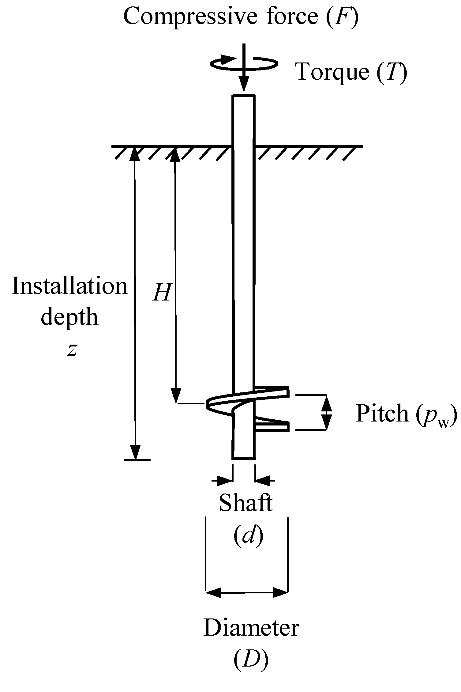
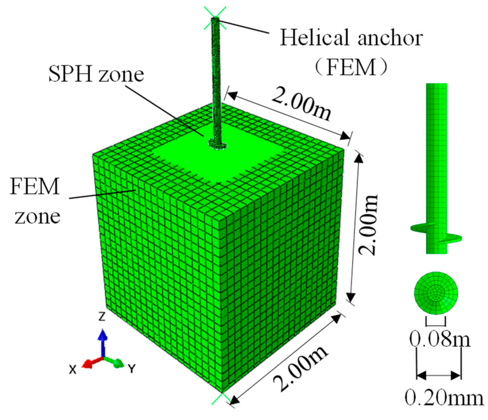
2. Establishment of SPH-FEM Model

SPH is a mesh-free particle method based on the Lagrangian description, which utilizes a set of arbitrarily distributed particles to solve integral equations or partial differential equations with complex boundary conditions, thereby obtaining accurate and stable numerical solutions. This method is particularly adept at addressing problems involving large deformations. Compared to other mesh-free methods, such as the Material Point Method (MPM), SPH offers two notable advantages in simulating the installation mechanism of piles. Firstly, SPH does not rely on a background mesh, allowing for more effective use of techniques like FEM to simulate soil far from the penetration area, thereby reducing computational costs and improving the accuracy of calculations in areas of small deformation. Secondly, as a well-established technique, SPH has been integrated into major commercial software packages like ABAQUS 6.14 and LSDYNA R14.0.0 [12]. The SPH-FEM coupling method proposed in this paper for simulating the installation process of helical anchor foundations is implemented in ABAQUS 6.14/EXPLICIT.

2.1. Computational Model and Material Parameters

The SPH-FEM coupled computational model is shown in Figure 2. For regions distant from the anchor’s penetration area, the FEM is employed for modeling, while the SPH method is used for the penetration zone and the surrounding soil. In the element type setting module of the ABAQUS software, both FEM elements and SPH particles can be defined. In this study, the FEM element type C3D8R is selected, and SPH particles are represented as PC3D elements within ABAQUS. The anchor plate diameter, D, is set to 0.20 m; the anchor plate thickness, t, is set to 0.01 m; the shaft diameter, d, is set to 0.08 m; the pitch of the helix, p_w, is provided in two sizes of 0.06 m and 0.08 m (Figure 2 shows the p_w = 0.08 m only); the length of the anchor rod is 1.50 m; and the distance from the center of the anchor plate to the bottom of the shaft is 0.08 m.

To avoid boundary effects, the size of the soil is set to 2 m × 2 m × 2 m. As shown in Figure 2, the whole soil region is divided into two parts: the SPH region and the FEM region. The size of the SPH region is 1 m × 1 m × 2 m, which is located in the middle of the whole model, and the rest is the FEM region. The contact surface between the SPH region and the FEM region is “tied” together using the “Tie Constraint” command, preventing any relative movement. A total of 128,000 uniformly distributed SPH particles are generated within the SPH region, while the FEM region is meshed using the C3D8R elements, totaling 6000 elements. The helical anchor is also discretized using the C3D8R elements, with a total of 2013 elements.

The soil parameters are selected from the literature [13], which are homogeneous dense sand, and the helical anchor is made of steel. The specific material parameters are shown in

Table 1. Parameters of helical anchor and soil.

Material Type	Young’s Modulus E (MPa)	Poisson’s Ratio ν (-)	Internal Friction Angle φ (°)	Dilatancy Angle ψ (°)	Density ρ (kg/m3)
Helical Anchor	2.06 × 105	0.30	-	-	7.85 × 103
Soil	60.00	0.25	37.00	7.00	1.69 × 103

. The stiffness of the helical anchor is much greater than that of the soil, and it is approximated as a rigid body in the model. The soil is characterized using the Mohr–Coulomb elastoplastic constitutive model. The contact properties between the helical anchor and the soil are set to general contact, with the normal behavior of the contact surface selected as “hard contact” and the tangential behavior as “penalty”. The friction angle δ between the pile and the soil is taken as 3/4 φ (φ is the internal friction angle of the soil) [8], and the coefficient of friction is taken as tan φ = 0.47.

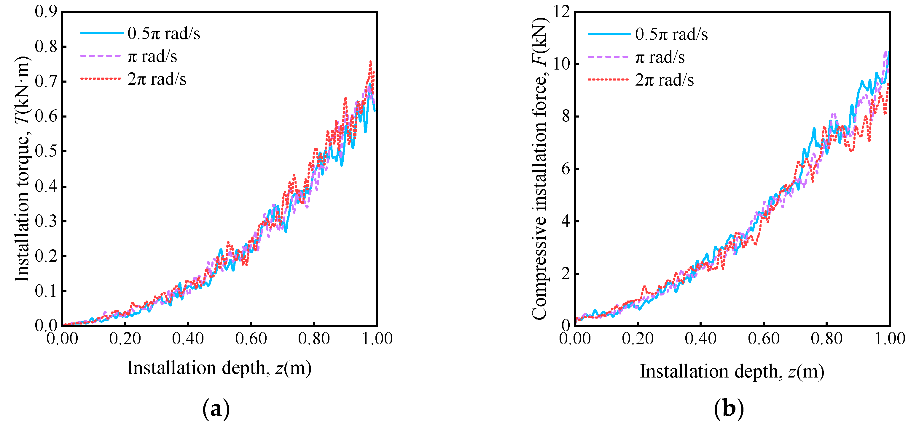
2.2. Initial Boundary Conditions and Sensitivity Analysis of Installation Speed

The SPH-FEM computational model is set up with a total of three analysis steps: the first step simulates geostatic stress equilibrium, the second step simulates the installation process of the helical anchor, and the third step simulates the uplift bearing process of the helical anchor.

The geostatic stress equilibrium is achieved by modifying key words. The vertical stress is determined by the height and unit weight of the soil, while the horizontal stress is determined based on the soil pressure coefficient K₀ and the vertical stress, where K₀ = 1-sinφ. The displacement boundary conditions for the soil are set as follows: the two lateral boundaries perpendicular to the x-direction restrict movement in the x-direction, the two lateral boundaries perpendicular to the y-direction restrict movement in the y-direction, and the bottom boundary of the soil model restricts movement in all three x, y, and z directions. The upper surface is free and unconstrained.

The movement of the helical anchor is controlled by a reference point at its top. During the installation process, a constant rotational speed is applied to the reference point while maintaining the anchor body in a vertical downward motion (with lateral displacement constrained) until the helical anchor is installed to the specified depth. In field construction, the typical rotation speed for the installation of helical anchors is 10~30 rpm. However, in the explicit dynamics module of ABAQUS, the duration of the analysis step is set to the actual physical process time. If the typical rotation speed is directly used, it will result in excessively long analysis steps, which in turn leads to significant computational costs. To reduce computation time, the rotation speed adopted in this paper is higher than the typical speed in the specifications. To ensure that the simulation rotation speed is selected appropriately, ensuring that the installation process is a quasi-static process, a sensitivity analysis of the rotation speed was conducted before the formal calculations using the SPH-FEM model.

Three rotational speeds of 0.5π rad/s, π rad/s, and 2π rad/s were used to simulate the installation of a helical anchor with an 0.08 m pitch, with an advance of one pitch per rotation (AR = 1.0), and the results are shown in Figure 3. It can be seen that as the installation depth increases, both the installation torque and compressive installation force show a gradual increase. Under the conditions of three different rotational speeds, the curves of installation torque versus installation depth and compressive installation force versus installation depth exhibit differences in the amplitude of oscillation, yet they maintain a consistent overall trend. This indicates that the impact of rotational speed on installation torque and compressive installation force is relatively minor. Considering computational cost and accuracy, a rotational speed of π rad/s was used for the subsequent simulations. Additionally, for the simulation of the pulling-up process of the helical anchor, displacement loading control was adopted with an upward pull displacement load of 0.2D applied at the reference point, and the loading speed was 2 × 10⁻³ m/s.

2.3. Model Verification

To verify the effectiveness of the SPH-FEM coupled model established in this paper, the variation curves of installation torque and force with installation depth obtained from the simulation were compared with the calculation results of the theoretical formula by Ghaly and Hanna [8], as shown in Figure 4. It can be observed that the simulation results from the SPH-FEM model are consistent with the theoretical formula-derived curves in terms of overall trends for both the variation in installation torque with installation depth and the variation in installation force with installation depth. However, there are some differences: the theoretical calculations yield smoother results, while the simulated curves exhibit certain fluctuations. These fluctuations are reasonable as they more closely resemble the actual installation process.

After the installation of the helical anchor foundation is completed, the ultimate uplift capacity is determined by applying a displacement at the reference point on the top of the anchor rod, and it is standardized as the uplift capacity factor N_r (N_r = Q_u/γAH, where Q_u is the ultimate uplift capacity, γ is the unit weight of the soil, A is the area of the anchor plate, and H is the depth of burial of the anchor plate). Figure 5 presents a comparison between the numerically simulated uplift capacity factor obtained in this study for the embedment ratios H/D of 4.6 and 5.6, and the theoretical calculations by Wang et al. [10] and Ghaly et al. [14]. It can be observed from the figure that at H/D = 4.6, the simulated uplift bearing capacity coefficient in this study is 30.9, and at H/D = 5.6, it is 41.5. In contrast, the theoretical values calculated by Wang et al. [10] are 35.5 and 45.3, and those by Ghaly et al. [14] are 33.6 and 45.2. Although the simulated values in this study are slightly lower than the theoretical values, the discrepancies are within 5%. Therefore, it can be concluded that the model used in this study for simulating the uplifting process is reasonable and feasible.

3. Simulation Results and Discussion

To study the effects of the AR on the installation force, torque, and uplift capacity of the helical anchor, two models of helical anchor foundations with different pitches (0.06 m and 0.08 m) were established. In these two models, the AR was set to 0.8, 1.0, 1.2, and 1.5, with an installation depth of 1.20 m for both.

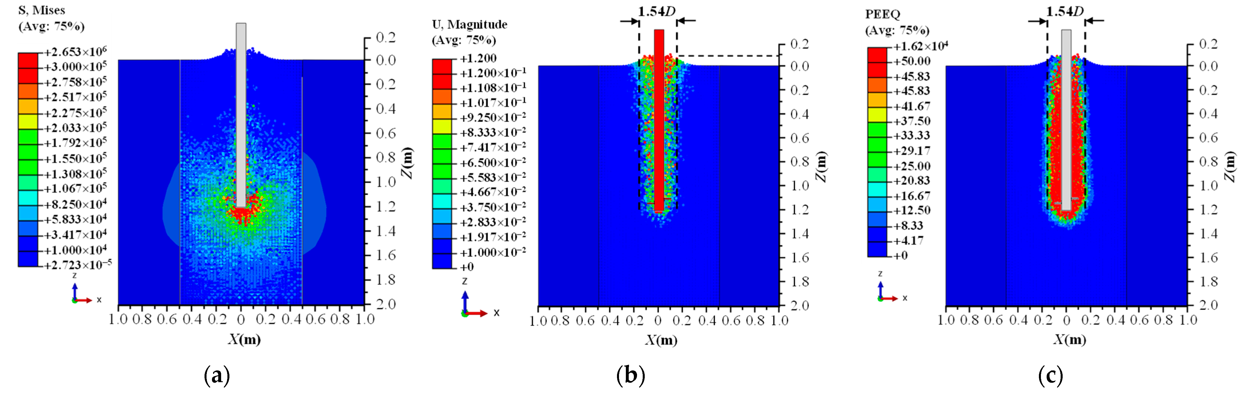
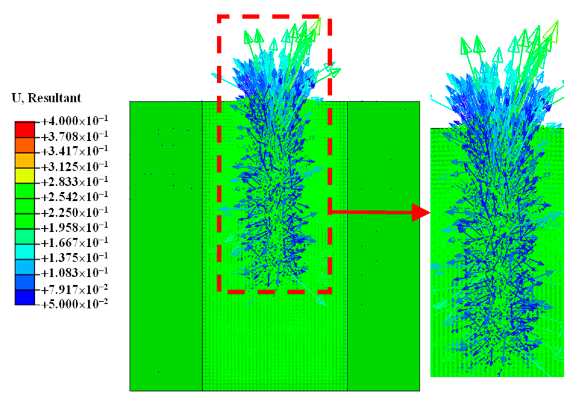
3.1. Disturbance to the Soil by Helical Anchor Installation

During the installation of the helical anchor, due to its unique combined motion of rotation and sinking, the soil around the anchor is subjected to the combined action of shear and compression, which leads to plastic deformation. To further explore the specific impact of this complex process on the soil, we select the 0.08 m pitch helical anchor as the research object and present the stress, displacement, and equivalent plastic strain PEEQ nephogram generated by the soil under the “pitch-matching” installation mode, as shown in Figure 6.

According to the stress distribution nephogram (Figure 6a), it can be found that during the installation process of the helical anchor foundation, the vertical load is transmitted to the soil through the anchor rod and anchor plate, forming a significant stress concentration area around the anchor. After the installation of the helical anchor foundation is completed, the stress within the soil is mainly distributed around the anchor plate and the end of the anchor rod, forming an asymmetric “V” shape. The boundary of the stress area is approximately 3D away from the anchor plate vertically, with the maximum load occurring directly below the anchor rod, reaching up to 2.653 MPa. For the soil more than 3D away from the anchor plate, the stress influence is minimal.

Further analysis of the displacement nephogram (Figure 6b) reveals that the soil experiencing displacement during the installation process is mainly concentrated near the projected area of the anchor plate. In conjunction with the research results proposed by Pérez et al. [15], the disturbed area can be determined to be a cylindrical volume with a diameter of about 1.54D. Within the cylinder, the displacement of the upper soil is significantly greater than that of the lower soil, especially within the 0.20 m range of the drilling point where there is a noticeable bulging of the soil, with the maximum bulging height reaching 0.09 m.

The equivalent plastic strain nephogram (Figure 6c) shows that after the installation of the helical anchor foundation, the soil within the disturbed zone has essentially entered the plastic stage, with the PEEQ values in the disturbed zone exceeding 50 (red areas in the figure). It is noteworthy that the plastic strain generated in the soil at the top of the disturbed zone is lower than that at the bottom. This may be attributed to the smaller overburden pressure on the top soil during the installation process, which results in a relatively lower load experienced during the screwing process.

To more intuitively reveal the movement characteristics of the soil in the disturbed zone, the displacement vector diagram of the soil in the disturbed zone is provided, as shown in Figure 7. It can be observed that the soil at the top of the disturbed zone has the largest displacement, and the direction of displacement is nearly vertical. With increasing depth, the direction of displacement gradually changes to horizontal. This indicates that after the helical anchor is installed to a certain depth, the soil displacement effect gradually becomes apparent, causing the diameter of the disturbed zone to be larger than the diameter of the anchor plate.

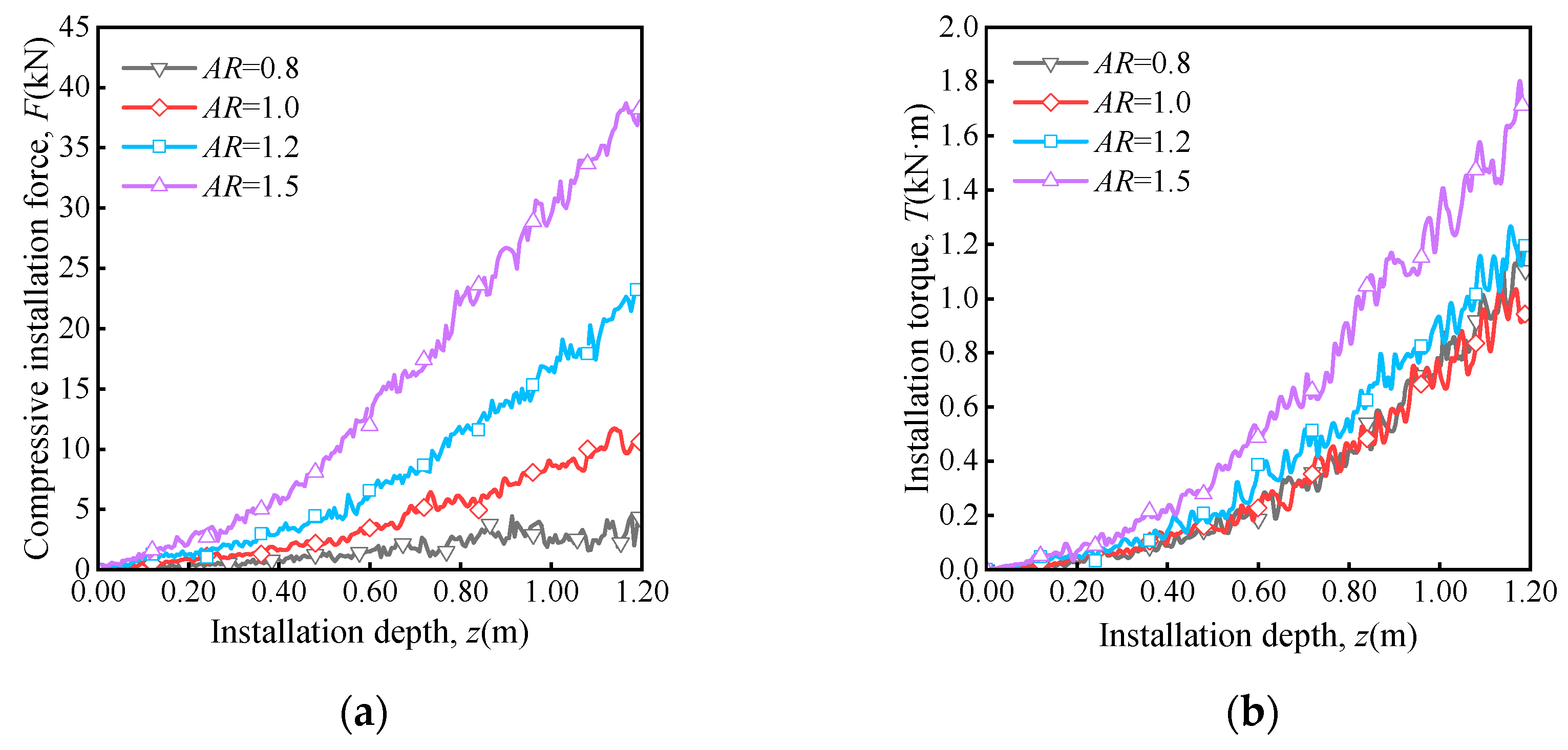
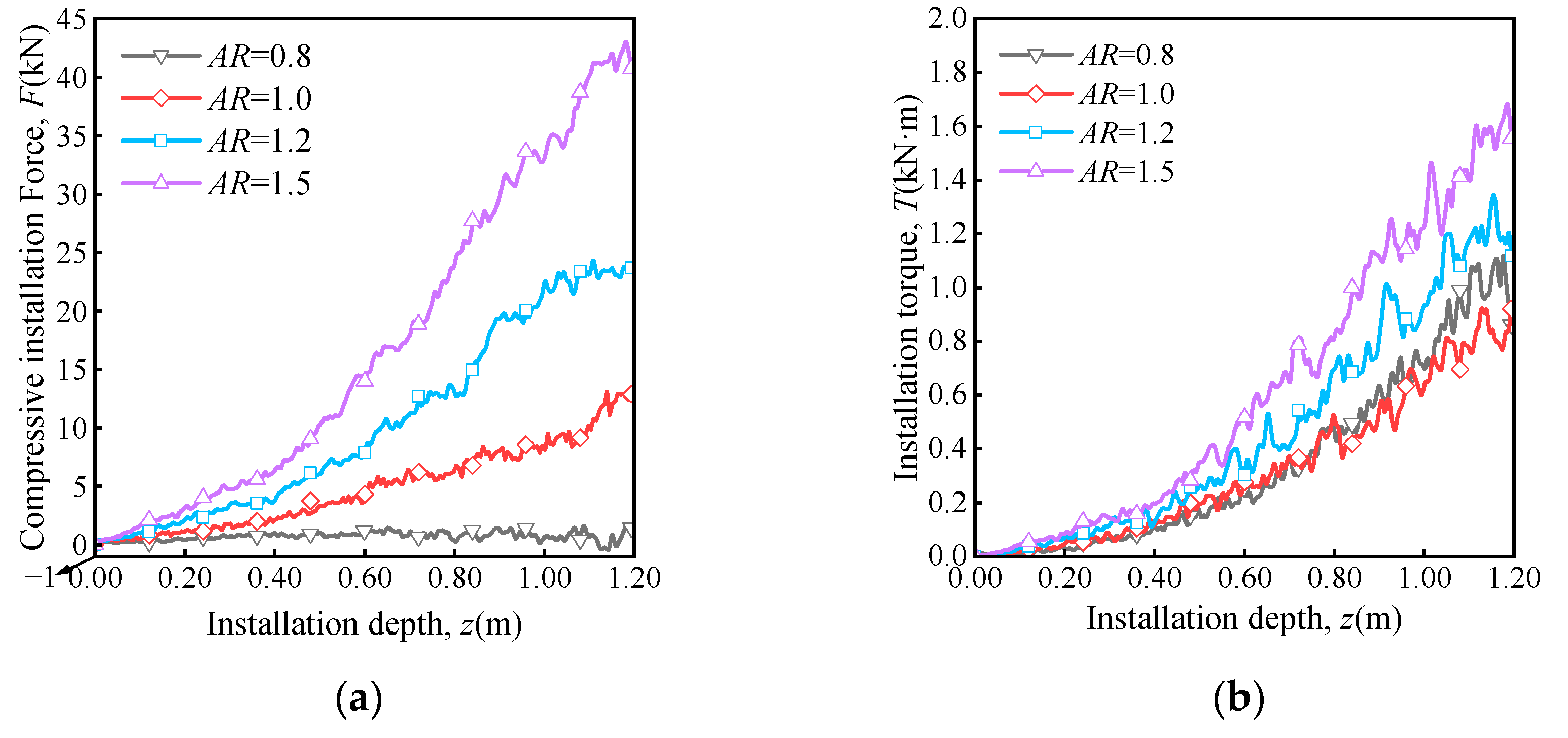
3.2. Influence of AR on Installation Force and Torque

To study the influence of the AR on the installation force and torque of the helical anchor foundations, Figure 8 and Figure 9, respectively, illustrate the relationship between the installation force F and installation torque T as a function of the installation depth z under various AR conditions for two helical anchors with different pitches.

From Figure 8 and Figure 9, it can be observed that both the installation force and torque gradually increase with the increase in installation depth, and the AR has a significant impact on both. Taking the installation depth z = 1.20 m as an example, compared to the “pitch-matched” installation mode (AR = 1.0), when a low advancement ratio (AR = 0.8) is used for installation, the required installation force decreases by an average of 94%, while the installation torque increases by an average of 13%. When a high advancement ratio (AR = 1.2, 1.5) is used for installation, the required installation force increases by an average of 94% and 234%, respectively, and the installation torque increases by an average of 28% and 69%.

Furthermore, it is noteworthy that for the helical anchor with a pitch of 0.08 m, compressive installation force were negative at the depths of 1.10 to 1.50 m when the AR was 0.8, a phenomenon that is consistent with the indoor experimental results of Wang et al. [10]. This indicates that the helical anchor foundation experienced a downward pull during the installation process. This phenomenon may be related to the special structure of the helical anchor plate. During installation, the helical anchor plate not only continuously shears the soil around the anchor but also lifts the soil above the plate, resulting in a downward reaction force from the soil on the plate. When the AR is low, this reaction force may be sufficient to cause the helical anchor to continue to screw into the soil, hence the installation pressure is zero or negative. This also explains why the helical anchor foundation can still screw into the soil at a slower speed when the compressive installation force provided by the installation equipment is insufficient.

Comparing the installation torque curves for AR = 0.8 and AR = 1.0 reveals that the torque at AR = 0.8 is slightly higher than at AR = 1.0 when the depth is greater than 1.00 m. This suggests that the effect of AR on the installation may also depend on the depth of the installation. For this purpose, the installation forces and torques at the depths of 0.40 m, 0.80 m, and 1.20 m for each AR were extracted and normalized against the forces and torques (F_1.0 and T_1.0) corresponding to the AR = 1.0 installation. The results are presented in Figure 10 and Figure 11.

Figure 10 shows that at each installation depth, there is a linear positive correlation between the installation force and AR, meaning that the installation force increases linearly with the increase in AR. The slope of the fitted line is defined as the influence coefficient of AR on the installation force. The fitting results indicate that the influence coefficient of AR on the installation force ranges from 3.9 to 4.7 and tends to increase with the installation depth.

Figure 11 shows that when a high AR is used for installation, there is also a linear positive correlation between the installation torque and AR at various depths. Similarly, the slope of the fitted line is defined as the influence coefficient of the AR on the installation torque. The fitting results show that the installation torque influence coefficient remains essentially unchanged with the increase in installation depth, being approximately 1.3 for the sandy soil used in this simulation. This value is significantly smaller than the influence coefficient of AR on the installation force, indicating that AR has a more pronounced effect on the installation force.

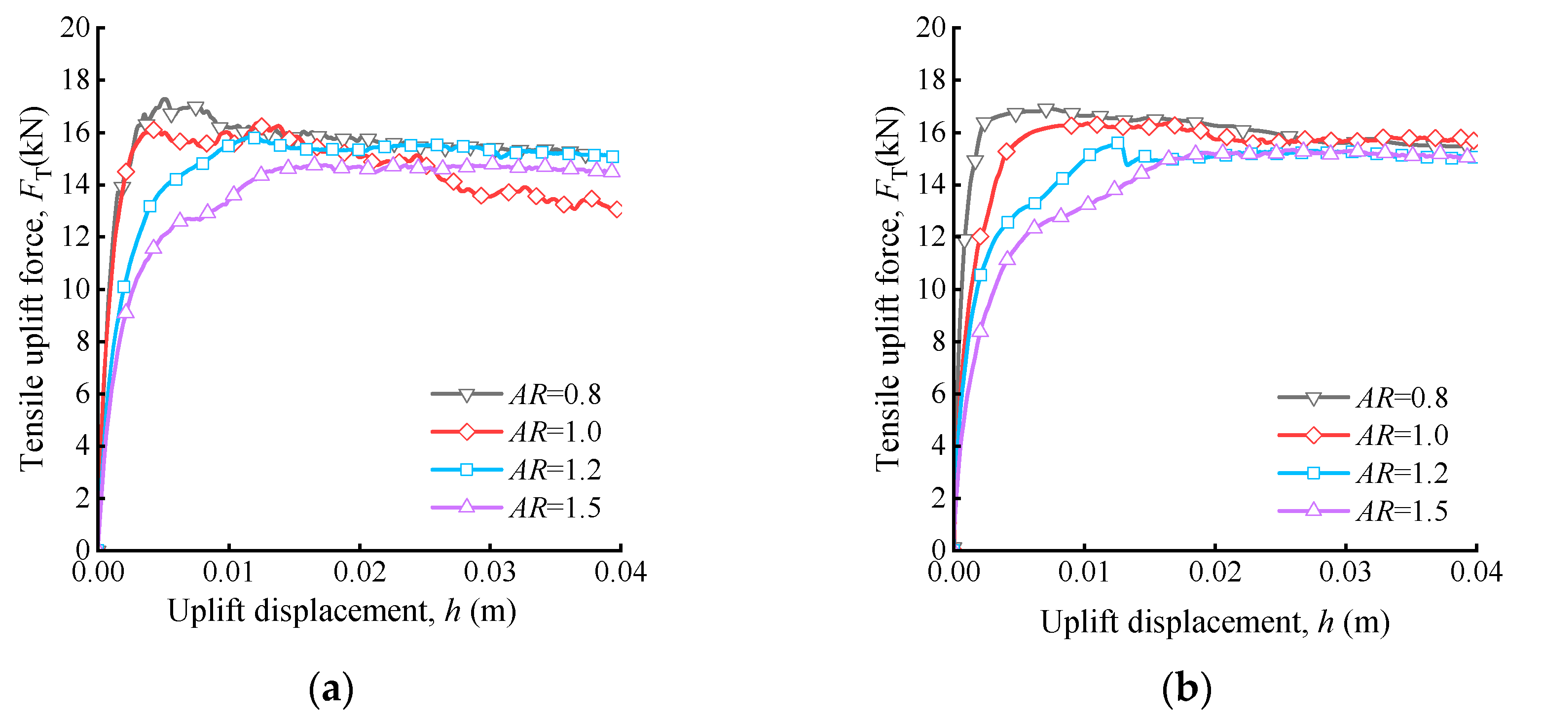
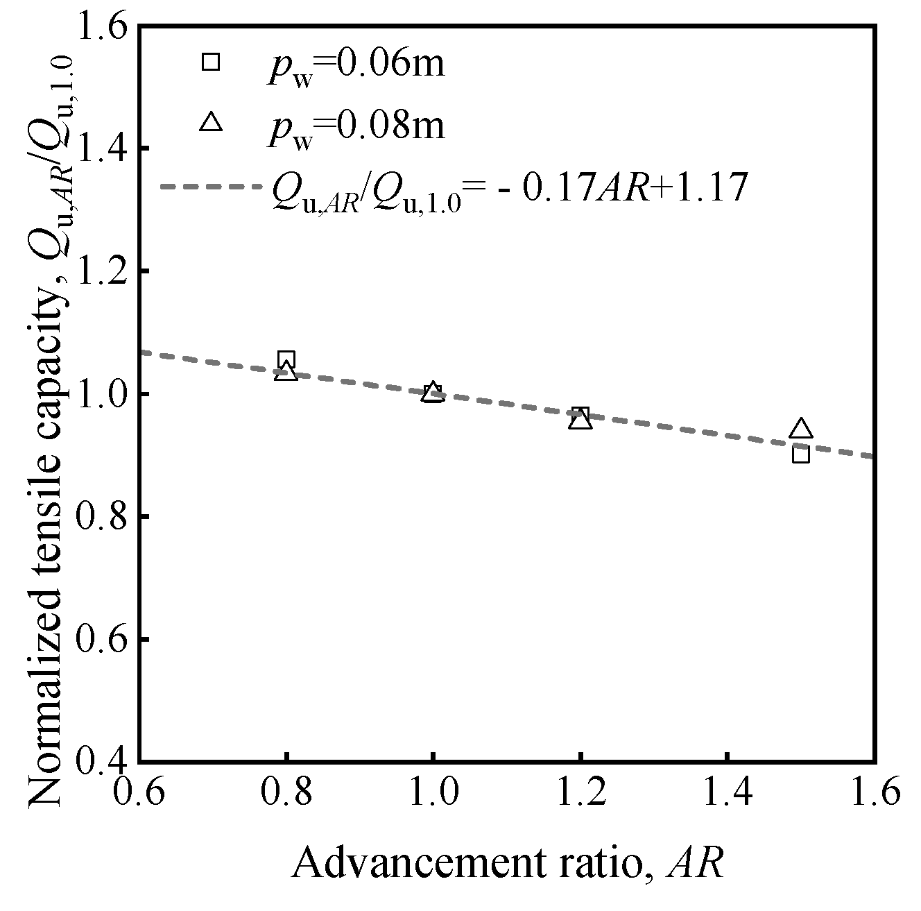
3.3. Influence of AR on the Uplift Bearing Capacity of Helical Anchor Foundations

After the installation of the helical anchor foundation is completed, a vertical displacement load with a speed of 2 × 10⁻³ m/s is applied to the reference point at the top of the anchor rod until 20% of the anchor plate diameter is pulled out. Figure 12 shows the load–displacement curves under various ARs during the uplifting process, with the vertical axis representing the uplift load F_T and the horizontal axis representing the uplift displacement h.

From Figure 12, it can be observed that as the uplift displacement increases, the uplift load initially increases rapidly, then slowly decreases, and gradually stabilizes. The initial slope of the curve can be used to characterize the stiffness of the soil. According to the characteristics of the curve, it can be found that as the AR increases, the initial slope of the curve tends to decrease. This indicates that an increase in the AR also increases the degree of soil disturbance.

To accurately assess the uplift performance of the helical anchor, the peak point of the load–displacement curve is determined as the ultimate uplift capacity Q_u of the helical anchor foundation. From Figure 12, it can be observed that when the AR = 0.8, the ultimate uplift capacity is the highest, about 5% higher than that when AR = 1.0. However, the displacement corresponding to the ultimate uplift capacity is essentially the same as that when AR = 1.0. As the AR increases, the ultimate uplift capacity gradually decreases, but the displacement corresponding to the ultimate uplift capacity increases. Taking the ultimate uplift capacity when AR = 1 as the basis, the ultimate uplift capacity under different ARs is normalized. The normalized ultimate uplift capacity Q_u,AR/Q_u,1.0 of each AR is shown in Figure 13.

From Figure 13, it can be observed that the normalized ultimate uplift capacity shows a linear negative correlation with the AR. The slope of the fitted line is defined as the influence coefficient of AR on the ultimate uplift capacity. The fitting results show that the influence coefficient of AR on the ultimate uplift capacity is only 0.17, indicating that the influence of AR on the ultimate uplift capacity is relatively small. However, this linear relationship is specific to the range of AR values studied. The goodness-of-fit index, χ², for the linear model is 0.852, providing a quantitative assessment of how well the model fits the data. It is important to note that while the linear fit may appear reasonable in small graphs, the actual fit may have limitations.

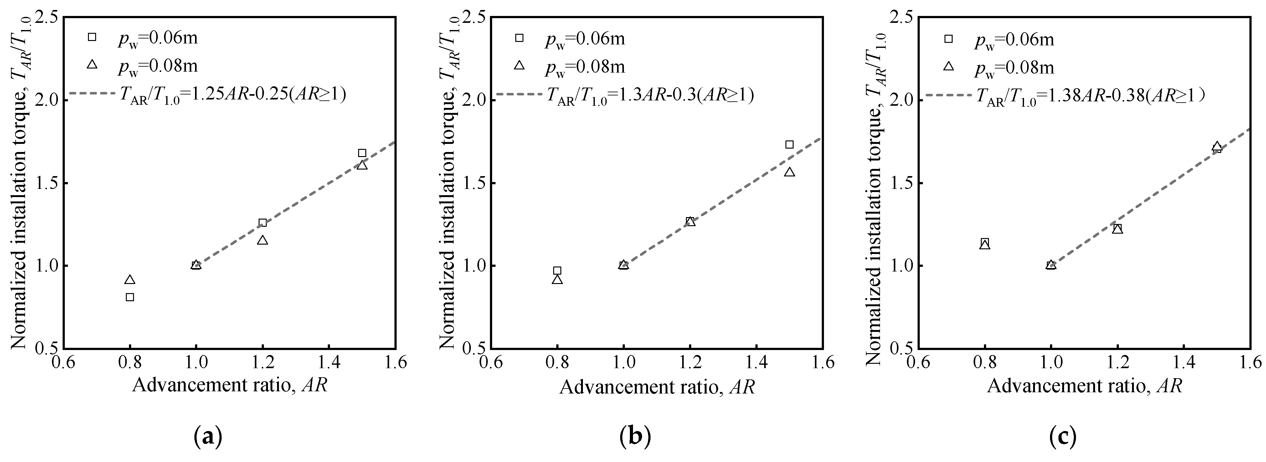
3.4. Influence of AR on the Torque Correlation Factor K_t

For the design and construction of helical anchors, accurately predicting their uplift capacity is crucial. In past research, Hoyt and Clemence [16] summarized empirical Formula (2) based on engineering experiments, which relates the axial load capacity of helical anchors to the final installation torque, with K_t being the torque correlation coefficient. Although there is no consensus among many scholars on the theoretical research results, this empirical formula is widely used in the industry for predicting the uplift capacity of helical anchors [17]. Additionally, according to a large number of field test results, Perko [6] points out that the value of K_t is not unique and is related to the shaft diameter d of the helical anchor, and proposed a formula for calculating K_t, as shown in Formula (3).

$$Q_u=K_{t}T$$

(2)

$$K_t=2.54d^{-0.9198}$$

(3)

In this paper, using Formula (2), the final installation torque T, and the uplift capacity Q_u obtained from Section 3.2 and Section 3.3, the K_t values under several ARs were calculated. These were compared with the K_t values obtained from Formula (3) and the K_t values from Tsuha’s experiments [18], as shown in Figure 14. It can be observed that the calculated K_t values in this paper range from 8.5 to 17.8 m⁻¹. The K_t value at AR = 1.0 is close to the results of Tsuha’s research and is lower than Perko’s theoretical calculation value of 25.9 m⁻¹. Therefore, using Perko’s theoretical K_t value would result in a significant overestimation of the uplift capacity.

Furthermore, Perko’s theoretical formula indicates that for a helical anchor with a certain shaft diameter, the K_t value is also predetermined and does not consider the impact of the installation method. However, as can be seen from Figure 14, the AR significantly affects the K_t value. Compared with AR = 1.0, the K_t value decreases by 8% at AR = 0.8, by 22% at AR = 1.2, and by 45% at AR = 1.5. Therefore, using the K_t value measured at an AR of 1.0 to predict the ultimate uplift capacity of the helical anchor under other ARs could lead to an overestimation, which may adversely affect the engineering project.

To accurately predict the uplift capacity of the helical anchor, it is recommended to monitor the AR during the installation and select the appropriate K_t value based on the actual AR when applying the empirical Formula (2) in actual engineering. This can avoid the prediction errors of the uplift capacity due to the improper selection of the K_t value, thus ensuring the safety of the project.

4. Conclusions

This paper is the first to employ the SPH-FEM to simulate the installation and extraction process of helical anchors in sandy soil foundations, analyzing the impact of the advancement ratio on the installation force, installation torque, uplift capacity, and torque correlation coefficient. The following principal conclusions have been reached:

(1)

The AR significantly influences the installation force and torque of the helical anchor. Compared to the “pitch-matched” (AR = 1.0) installation method, employing a high AR (AR = 1.2, 1.5) results in a significant increase in both installation force and torque, with the force increase being more pronounced than that of the torque. Conversely, using a low AR (AR = 0.8) for installation can significantly reduce the installation force, although the change in installation torque is relatively minor.

(2)

The ultimate uplift capacity of the helical anchor foundation is linearly and negatively correlated with the AR. At a low AR (AR = 0.8), the foundation achieves its maximum ultimate uplift capacity, which is approximately 4% higher than that obtained with the “pitch-matched” installation (AR = 1.0).

(3)

The AR affects the torque correlation coefficient K_t. The K_t value peaks when using the “pitch-matched” installation (AR = 1.0). Utilizing the K_t value determined at this AR to predict the ultimate uplift capacity of the helical anchor under other AR will likely result in an overestimation.

References

1. Lutenegger, A.J.; Tsuha, C.d.H. Evaluating installation disturbance from helical piles and anchors using compression and tension tests. In From Fundamentals to Applications in Geotechnics; IOS Press: Amsterdam, The Netherlands, 2015; pp. 373–381. [Google Scholar]
2. Yu, H.; Zhou, H.; Sheil, B.; Liu, H. Finite element modelling of helical pile installation and its influence on uplift capacity in strain softening clay. Can. Geotech. J. 2022, 59, 2050–2066. [Google Scholar] [CrossRef]
3. Annicchini, M.M.; Schiavon, J.A.; Tsuha, C.d.H.C. Effects of installation advancement rate on helical pile helix behavior in very dense sand. Acta Geotech. 2023, 18, 2795–2811. [Google Scholar] [CrossRef]
4. Davidson, C.; Brown, M.J.; Cerfontaine, B.; Al-Baghdadi, T.; Knappett, J.; Brennan, A.; Augarde, C.; Coombs, W.; Wang, L.; Blake, A. Physical modelling to demonstrate the feasibility of screw piles for offshore jacket-supported wind energy structures. Géotechnique 2022, 72, 108–126. [Google Scholar] [CrossRef]
5. BS 8004:2015; Code of Practice for Foundations. British Standards Institution: London, UK, 2015.
6. Perko, H.A. Helical Piles: A Practical Guide to Design and Installation; John Wiley & Sons: Hoboken, NJ, USA, 2009. [Google Scholar]
7. Al-Baghdadi, T. Screw Piles as Offshore Foundations: Numerical and Physical Modelling. Doctoral Thesis, University of Dundee, Dundee, UK, 2018. [Google Scholar]
8. Ghaly, A.; Hanna, A. Experimental and theoretical studies on installation torque of screw anchors. Can. Geotech. J. 1991, 28, 353–364. [Google Scholar] [CrossRef]
9. Shi, D.; Yang, Y.; Deng, Y.; Liu, W. Experimental study of the effect of drilling velocity ratio on the behavior of auger piling in sand. Rock Soil Mech. 2018, 39, 1981–1990. [Google Scholar] [CrossRef]
10. Wang, L.; Zhang, P.; Ding, H.; Tian, Y.; Qi, X. The uplift capacity of single-plate helical pile in shallow dense sand including the influence of installation. Mar. Struct. 2020, 71, 102697. [Google Scholar] [CrossRef]
11. Sharif, Y.U.; Brown, M.J.; Cerfontaine, B.; Davidson, C.; Ciantia, M.O.; Knappett, J.A.; Ball, J.D.; Brennan, A.; Augarde, C.; Coombs, W. Effects of screw pile installation on installation requirements and in-service performance using the discrete element method. Can. Geotech. J. 2021, 58, 1334–1350. [Google Scholar] [CrossRef]
12. He, H.; Karsai, A.; Liu, B.; Hammond III, F.L.; Goldman, D.I.; Arson, C. Simulation of compound anchor intrusion in dry sand by a hybrid FEM+ SPH method. Comput. Geotech. 2023, 154, 105137. [Google Scholar] [CrossRef]
13. Nagai, H.; Tsuchiya, T.; Shimada, M. Influence of installation method on performance of screwed pile and evaluation of pulling resistance. Soils Found. 2018, 58, 355–369. [Google Scholar] [CrossRef]
14. Ghaly, A.; Hanna, A.; Hanna, M. Uplift behavior of screw anchors in sand. I: Dry sand. J. Geotech. Eng. 1991, 117, 773–793. [Google Scholar] [CrossRef]
15. Perez, Z.A.; Schiavon, J.A.; Tsuha, C.d.H.C.; Dias, D.; Thorel, L. Numerical and experimental study on influence of installation effects on behaviour of helical anchors in very dense sand. Can. Geotech. J. 2018, 55, 1067–1080. [Google Scholar] [CrossRef]
16. Hoyt, R. Uplift capacity of helical anchors in soil. In Proceedings of the 12th International Conference on Soil Mechanics and Foundation Engineering, Rio De Janeiro, Brazil, 13–18 August 1989; pp. 1019–1022. [Google Scholar]
17. da Silva, B.O.; Hollanda Cavalcanti Tsuha, C.; Beck, A.T. A procedure to estimate the installation torque of multi-helix piles in clayey sand using SPT data. Int. J. Civ. Eng. 2021, 19, 1357–1368. [Google Scholar] [CrossRef]
18. Tsuha, C.d.H.C.; Aoki, N. Relationship between installation torque and uplift capacity of deep helical piles in sand. Can. Geotech. J. 2010, 47, 635–647. [Google Scholar] [CrossRef]
Figure 1. Schematic diagram of helical anchor foundation installation.
Applsci 14 07672 g001
Figure 2. SPH-FEM computational model.
Applsci 14 07672 g002
Figure 3. Curves illustrating the variation in installation torque and compressive installation force with installation depth at different rotational speeds. (a) Installation torque T vs. installation depth z. (b) Compressive installation force F vs. installation depth z.
Applsci 14 07672 g003
Figure 4. Comparison of simulated and theoretical values of installation torque and compressive installation force. (a) Comparison of installation torque. (b) Comparison of compressive installation force, Ghaly & Hanna, 1991 [8].
Applsci 14 07672 g004
Figure 5. Comparison of the uplift capacity factor for different embedment depth ratios, Ghaly et al., 1991 [14]; Wang et al., 2019 [10].
Applsci 14 07672 g005
Figure 6. Disturbance from stress, displacement magnitude, and PEEQ in soil after helical anchor installation. (a) Stress nephogram (Pa). (b) Displacement magnitude nephogram (m). (c) PEEQ nephogram (-).
Applsci 14 07672 g006
Figure 7. Resultant soil displacement vector diagram in disturbed area (m).
Applsci 14 07672 g007
Figure 8. Relationship between compressive installation force and installation torque versus installation depth for a pitch of 0.06 m (pw = 0.06 m). (a) Compressive installation force F vs. depth z. (b) Installation torque T vs. depth z.
Applsci 14 07672 g008
Figure 9. Relationship between compressive installation force and installation torque versus installation depth for a pitch of 0.08 m (pw = 0.08 m). (a) Installation force F vs. depth z. (b) Installation torque T vs. depth z.
Applsci 14 07672 g009
Figure 10. Results of the influences of AR on the normalized compressive installation force for different values of the depth of installation z. (a) z = 0.40 m. (b) z = 0.80 m. (c) z = 1.20 m.
Applsci 14 07672 g010
Figure 11. Results of the influence of AR on the normalized installation torque for different values of the depth of installation z. (a) z = 0.40 m. (b) z = 0.80 m. (c) z = 1.20 m.
Applsci 14 07672 g011
Figure 12. Uplift stage force–displacement curves. (a) pw = 0.06 m. (b) pw = 0.08 m.
Applsci 14 07672 g012
Figure 13. Results of the influence of AR on normalized tensile capacity.
Applsci 14 07672 g013
Figure 14. Comparison of calculated torque capacity correlation factor Kt at various ARs with Tsuha (2010) [18] and Perko’s (2009) [6] results.
Applsci 14 07672 g014