

Sensor Fault Detection and Classification Using Multi-Step-Ahead Prediction with an Long Short-Term Memoery (LSTM) Autoencoder

Abstract
:1. Introduction
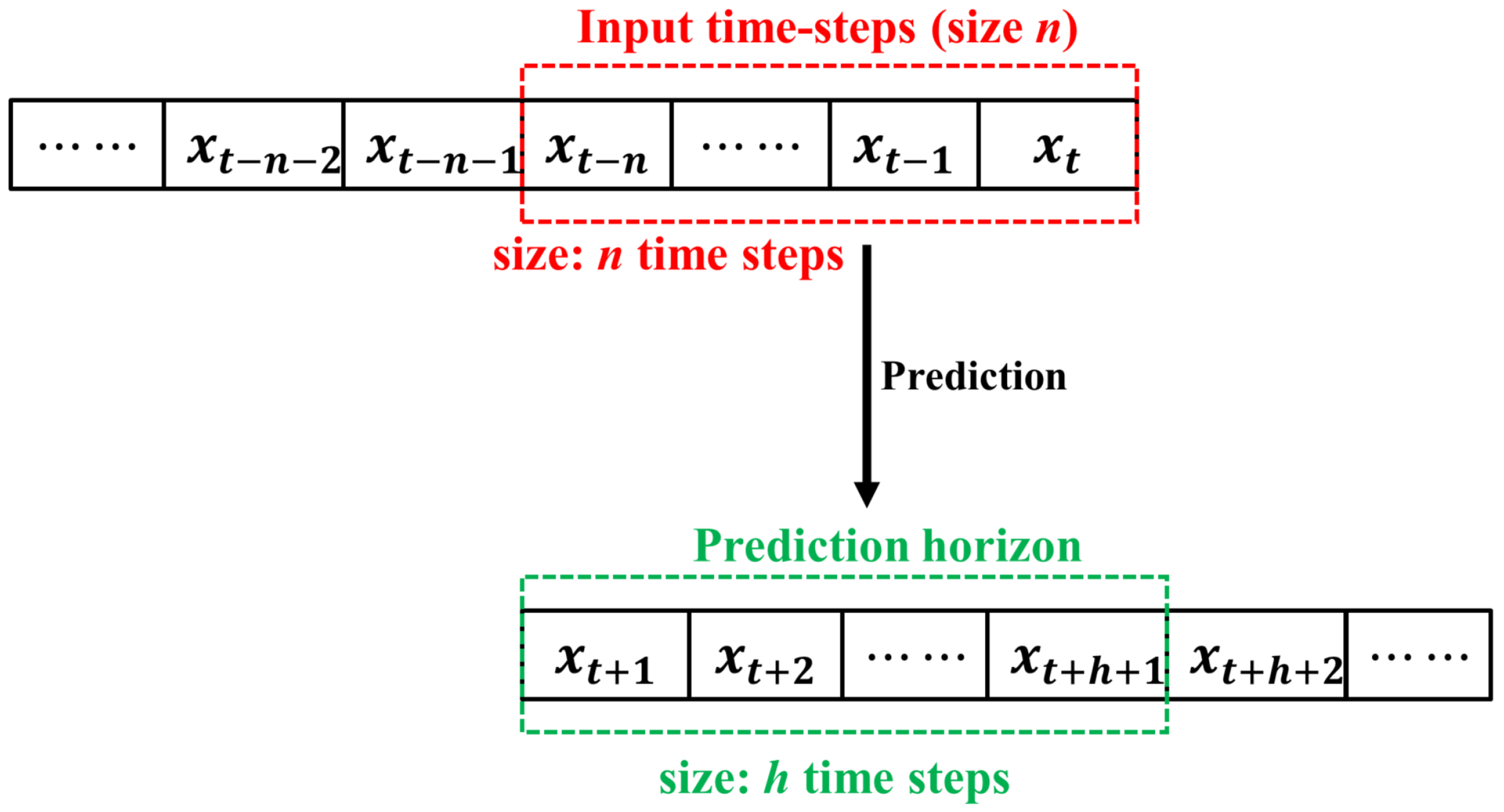
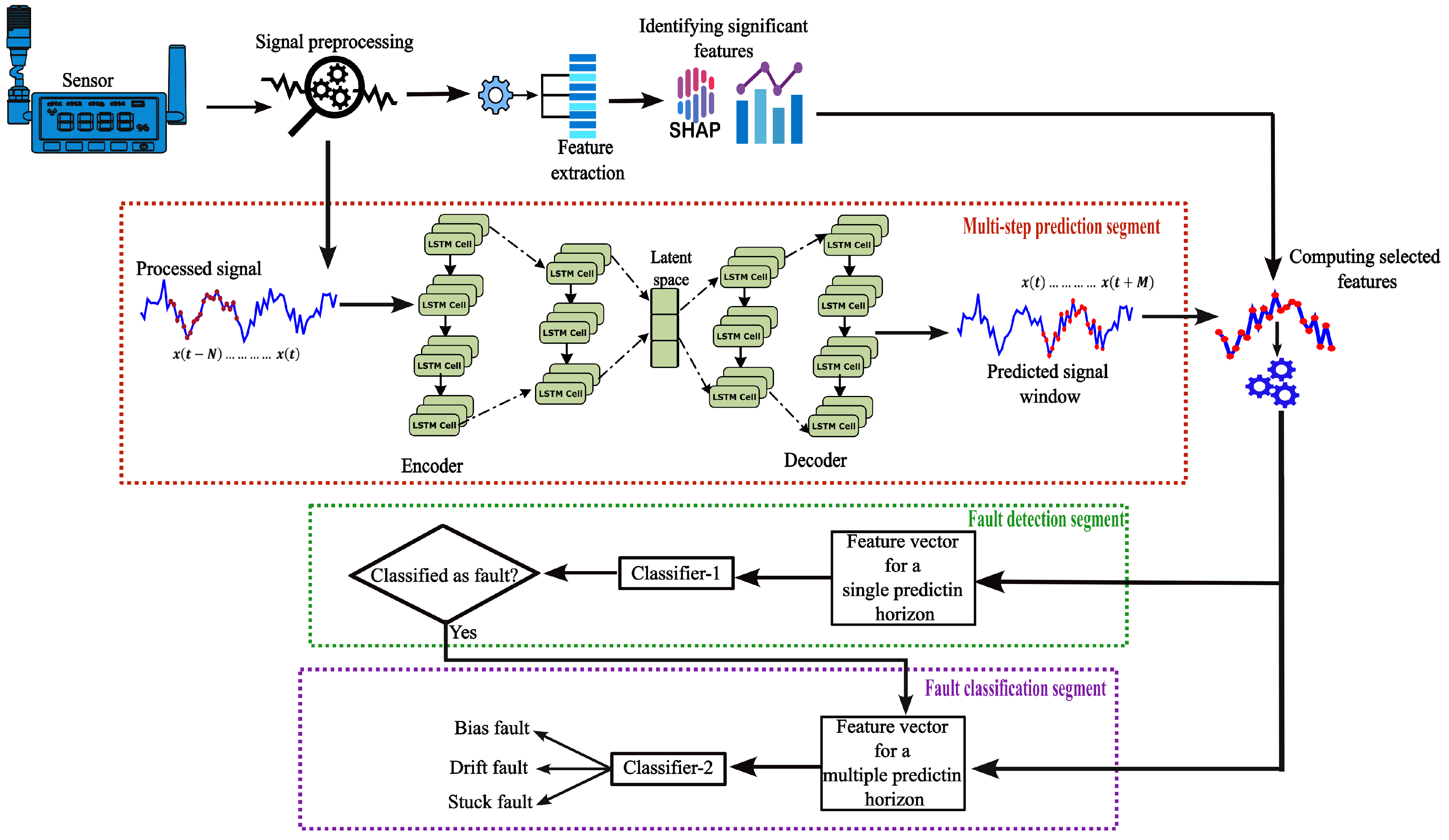
- A Long Short-Term Memory autoencoder (LSTM AE)-based univariate multi-step-ahead forecasting approach is proposed for sensor fault detection and classification. This method uses only normal sensor data for training.
- A feature extraction step is integrated into the prediction model to enable the detection of multiple types of faults. Additionally, three influential statistical features are reported that better represent bias, drift, and stuck faults in sensors.
- Results obtained from two different datasets are presented to demonstrate the functionality of the proposed approach.
2. Related Works
3. Materials and Methods
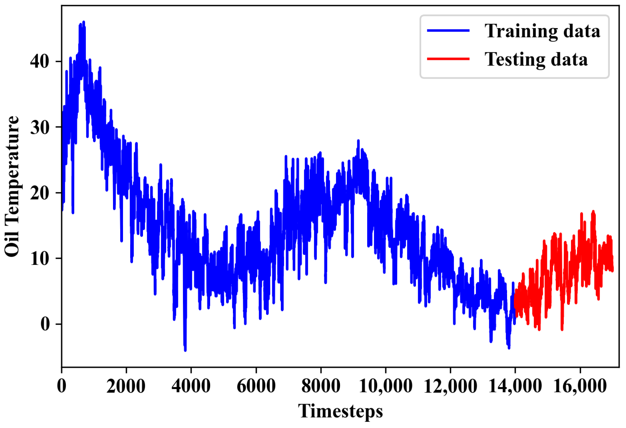
3.1. Datasets
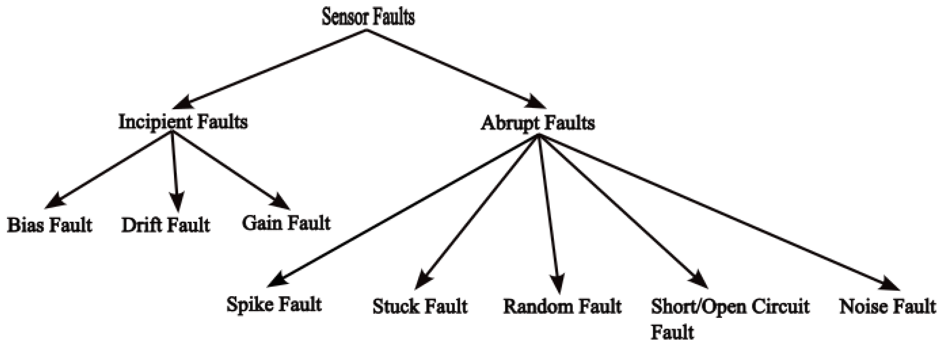
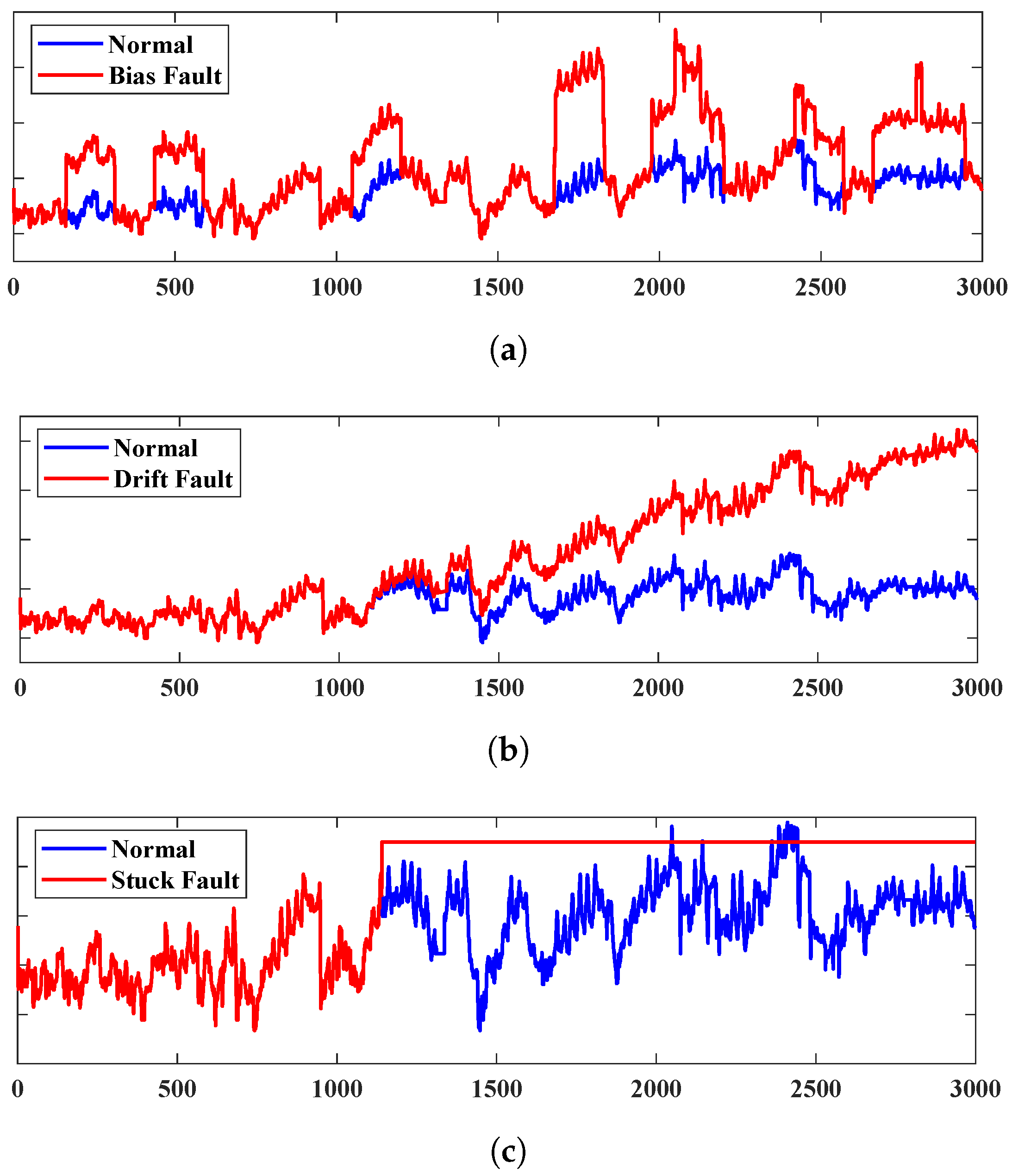
3.1.1. Bias Fault
3.1.2. Drift Fault
3.1.3. Stuck Fault
3.2. Signal Pre-Processing:
3.3. Feature Importance Analysis
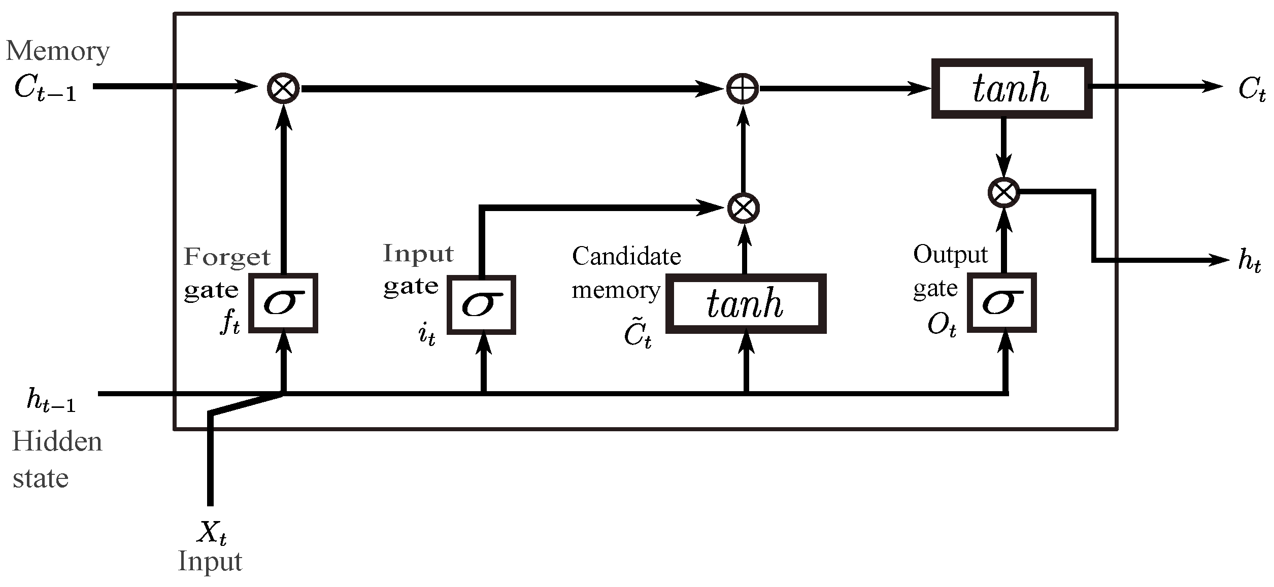
3.4. Long Short-Term Memory
3.5. LSTM Autoencoder
3.6. Fault Detection and Classification
| Algorithm 1 Multi-step prediction-based fault detection and classification. |
| Inputs: Training data: Time series sequence with data points, , Encoder: , Decoder: , Window size: , Prediction horizon: Outputs: Decision on fault detection and fault type Training Autoencoder: Create input and output sequences for do end for for Each training epochs do Encoder output: Decoder output: Calculate loss: Optimize the model parameters, : end for Prediction, Fault detection and classification: Predict the output sequence: Compute the four selected features: Fault detection: = if then Classify the fault type: = end if Return: Fault detection decision: Fault classification result: |
4. Results and Discussion
4.1. Feature Selection Using SHAP
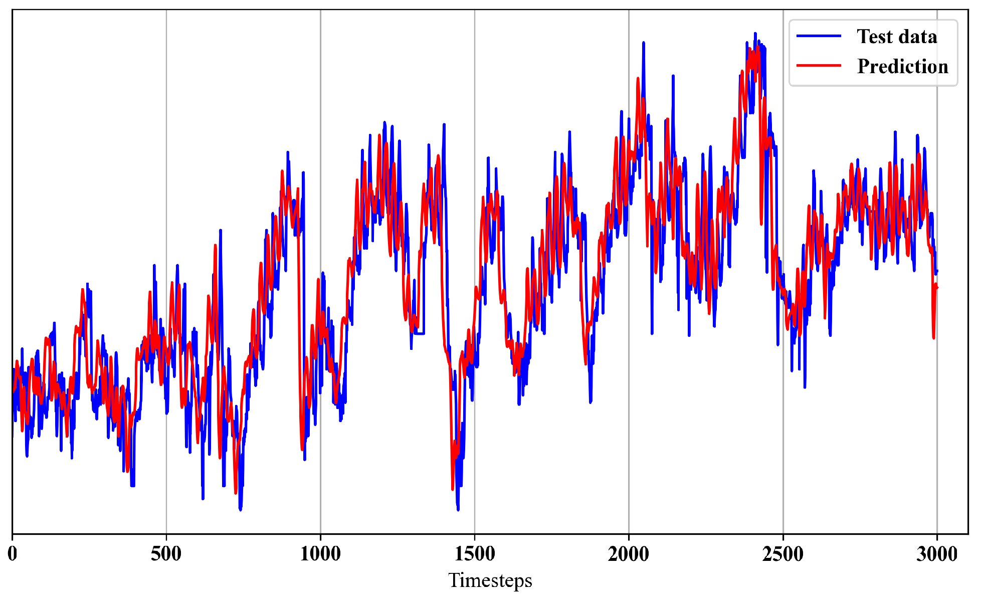
4.2. Multi-Step-Ahead Prediction by the Autoencoder
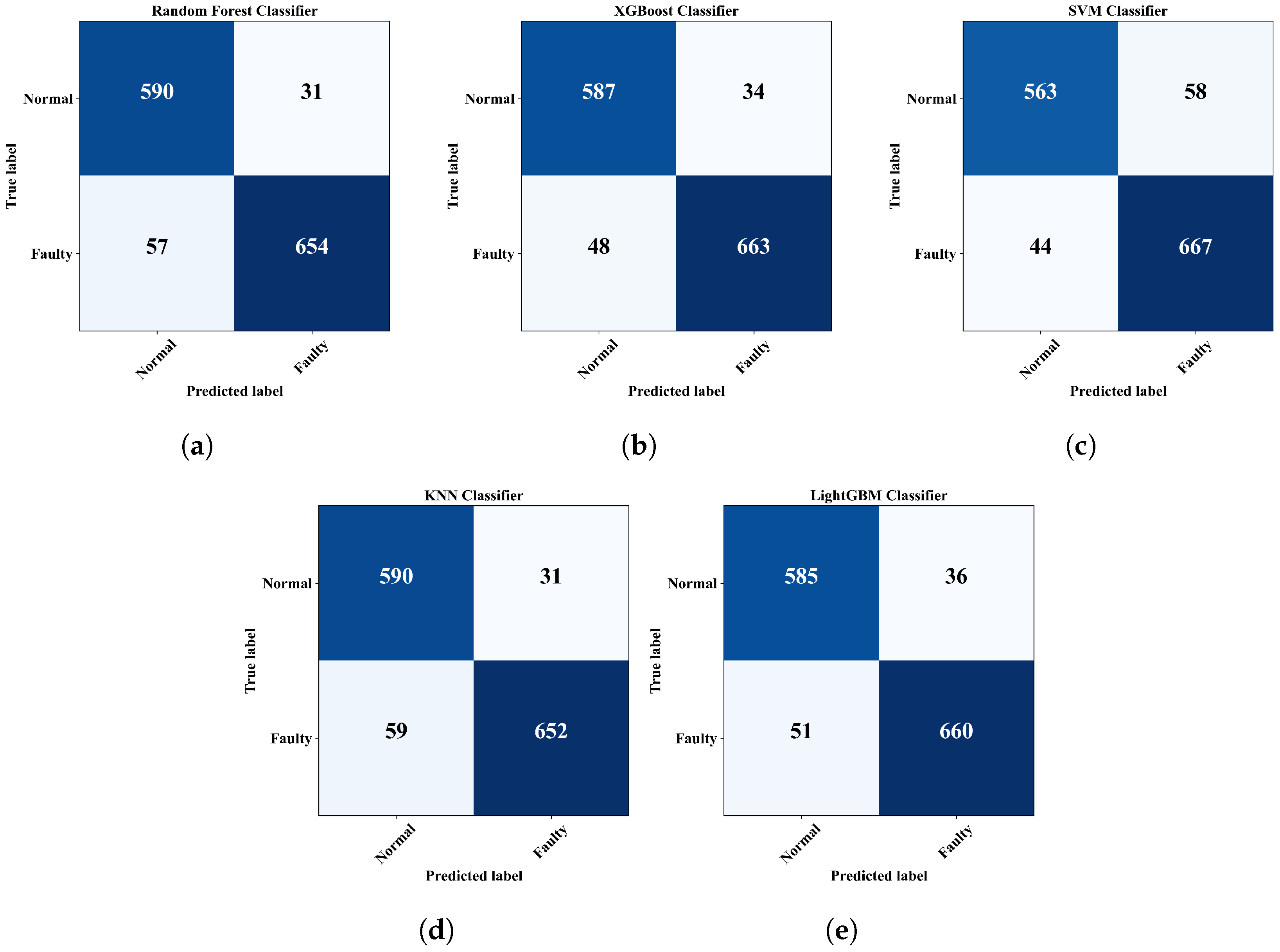
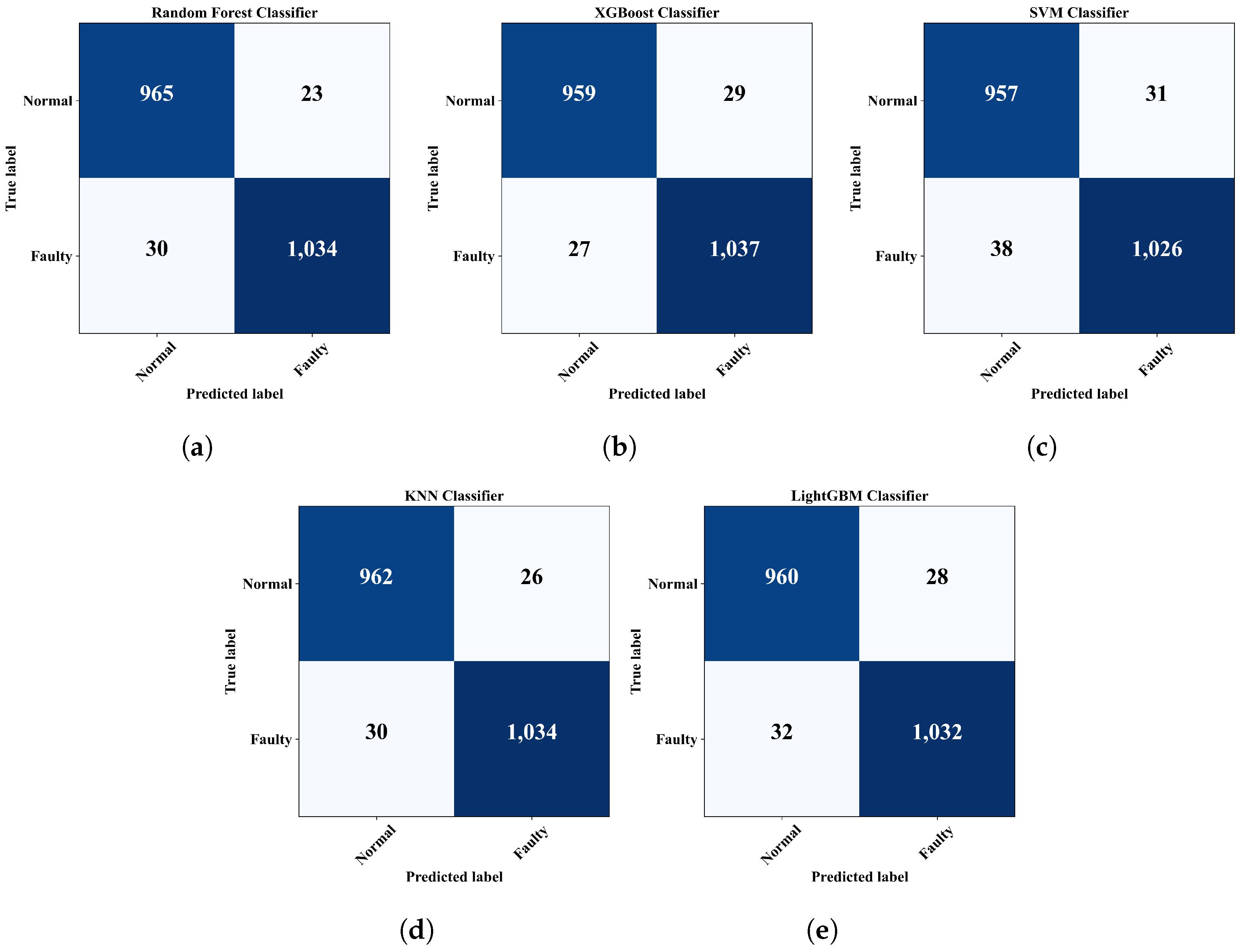
4.3. Sensor Fault Detection
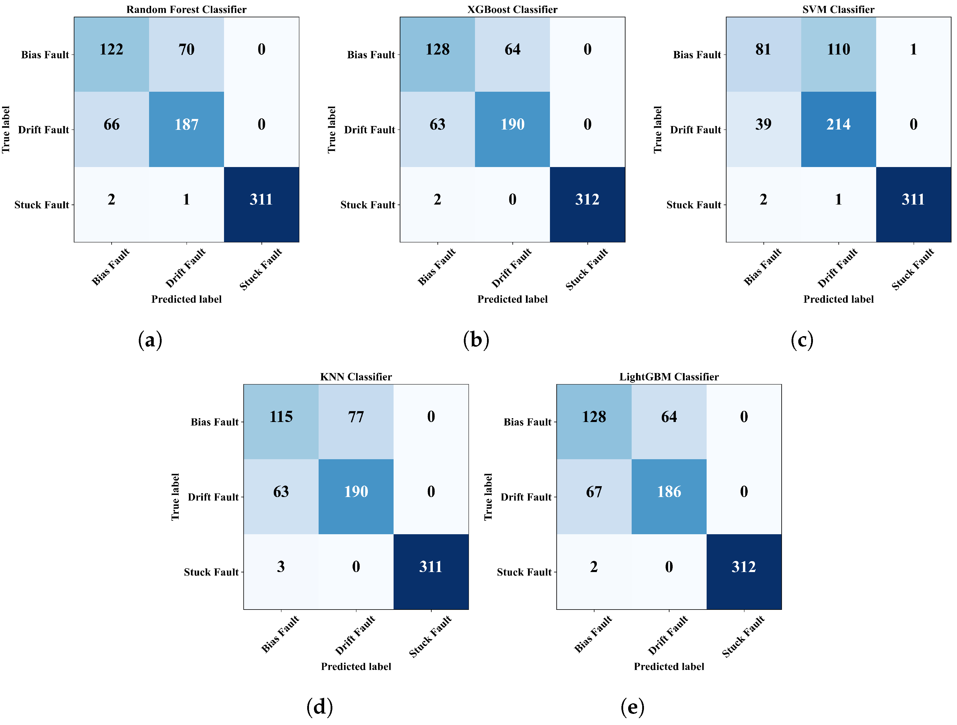
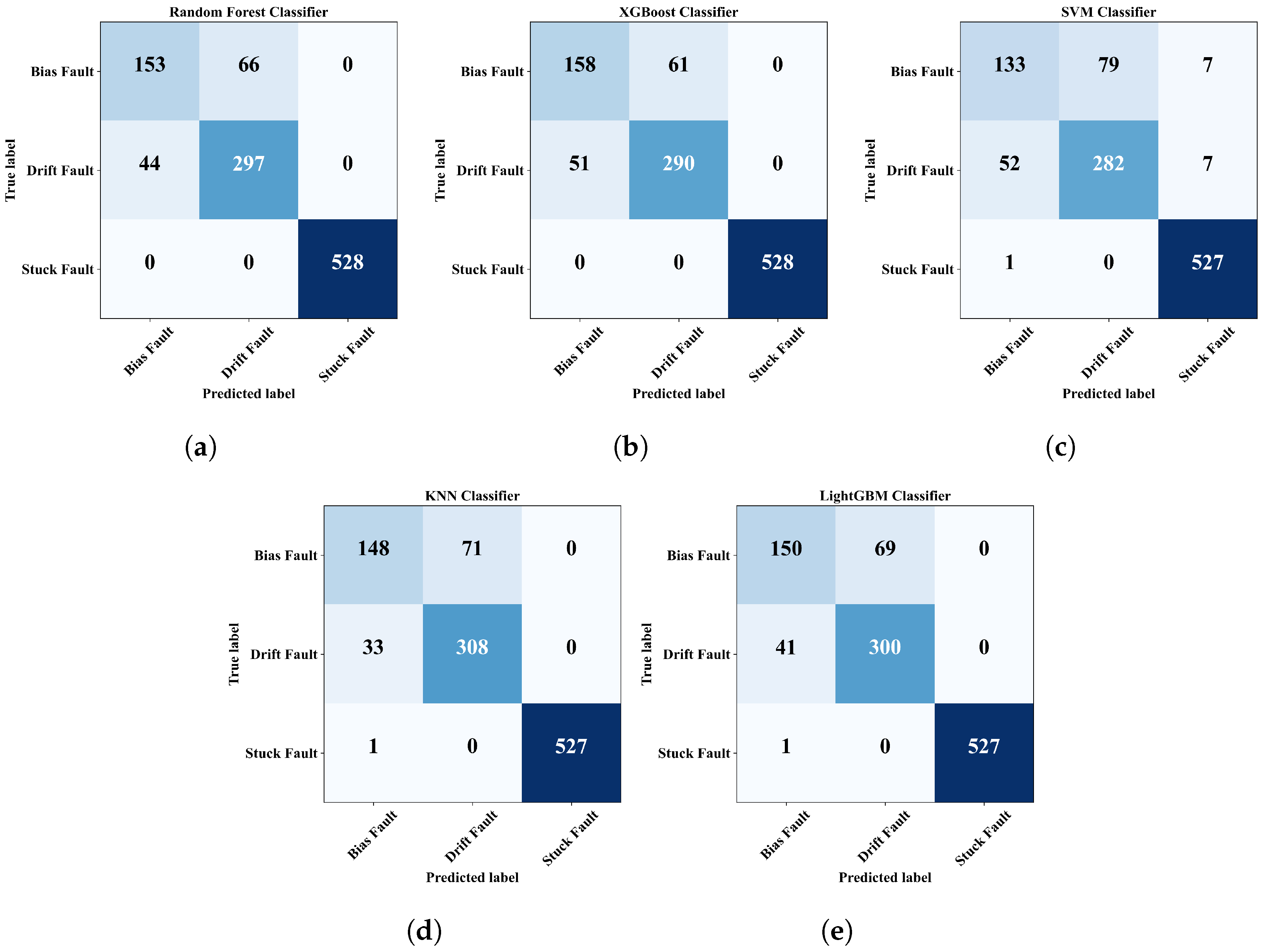
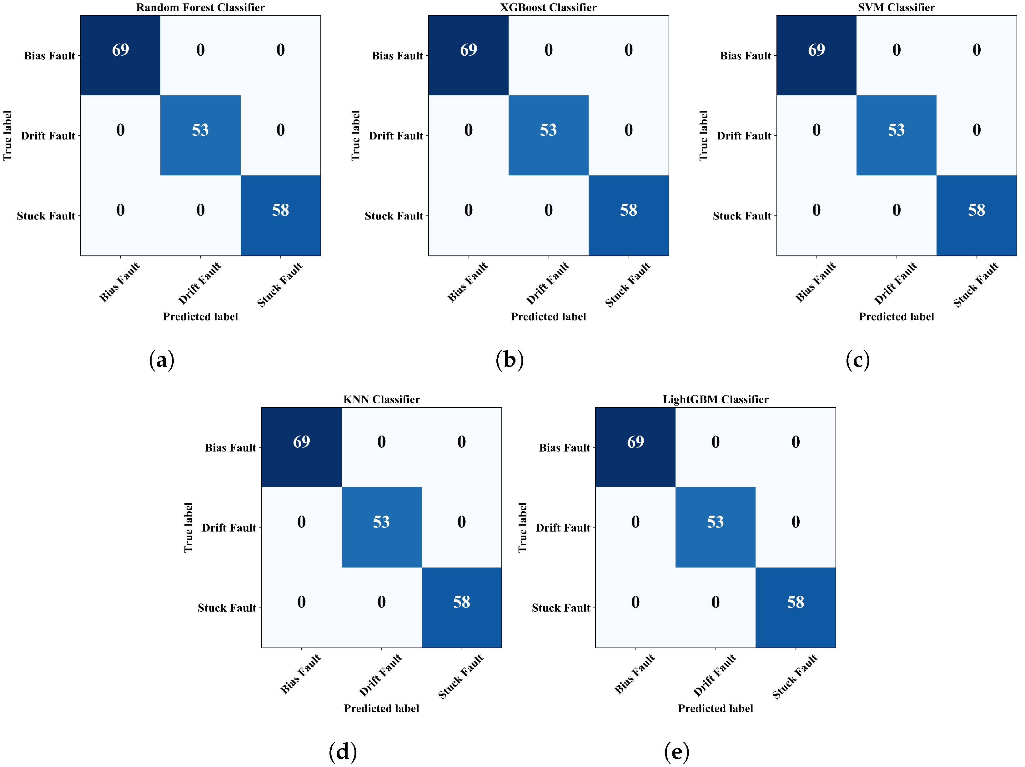
4.4. Fault Classification
5. Conclusions
Author Contributions
Funding
Institutional Review Board Statement
Informed Consent Statement
Data Availability Statement
Conflicts of Interest
References
- Famá, F.; Faria, J.N.; Portugal, D. An IoT-based interoperable architecture for wireless biomonitoring of patients with sensor patches. Internet Things 2022, 19, 100547. [Google Scholar] [CrossRef]
- Filho, I.d.M.B.; Aquino, G.; Malaquias, R.S.; Girão, G.; Melo, S.R.M. An IoT-Based Healthcare Platform for Patients in ICU Beds During the COVID-19 Outbreak. IEEE Access 2021, 9, 27262–27277. [Google Scholar] [CrossRef]
- Forcén-Muñoz, M.; Pavón-Pulido, N.; López-Riquelme, J.A.; Temnani-Rajjaf, A.; Berríos, P.; Morais, R.; Pérez-Pastor, A. Irriman platform: Enhancing farming sustainability through cloud computing techniques for irrigation management. Sensors 2021, 22, 228. [Google Scholar] [CrossRef] [PubMed]
- Mendes, J.; Peres, E.; Neves dos Santos, F.; Silva, N.; Silva, R.; Sousa, J.J.; Cortez, I.; Morais, R. VineInspector: The vineyard assistant. Agriculture 2022, 12, 730. [Google Scholar] [CrossRef]
- Ahmed, M.A.; Gallardo, J.L.; Zuniga, M.D.; Pedraza, M.A.; Carvajal, G.; Jara, N.; Carvajal, R. LoRa based IoT platform for remote monitoring of large-scale agriculture farms in Chile. Sensors 2022, 22, 2824. [Google Scholar] [CrossRef]
- Bates, H.; Pierce, M.; Benter, A. Real-time environmental monitoring for aquaculture using a LoRaWAN-based IoT sensor network. Sensors 2021, 21, 7963. [Google Scholar] [CrossRef]
- Khan, F.; Siddiqui, M.A.B.; Rehman, A.U.; Khan, J.; Asad, M.T.S.A.; Asad, A. IoT based power monitoring system for smart grid applications. In Proceedings of the 2020 International Conference on Engineering and Emerging Technologies (ICEET), Lahore, Pakistan, 22–23 February 2020; pp. 1–5. [Google Scholar]
- Shashank, A.; Vincent, R.; Sivaraman, A.K.; Balasundaram, A.; Rajesh, M.; Ashokkumar, S. Power analysis of household appliances using IoT. In Proceedings of the 2021 International Conference on System, Computation, Automation and Networking (ICSCAN), Puducherry, India, 30–31 July 2021; pp. 1–5. [Google Scholar]
- Kumaran, K. Power theft detection and alert system using IOT. Turk. J. Comput. Math. Educ. (TURCOMAT) 2021, 12, 1135–1139. [Google Scholar]
- Alam, T. Cloud-based IoT applications and their roles in smart cities. Smart Cities 2021, 4, 1196–1219. [Google Scholar] [CrossRef]
- Padmanaban, S.; Samavat, T.; Nasab, M.A.; Nasab, M.A.; Zand, M.; Nikokar, F. Electric vehicles and IoT in smart cities. In Artificial Intelligence-Based Smart Power Systems; John Wiley & Sons, Inc.: Hoboken, NJ, USA, 2023; pp. 273–290. [Google Scholar]
- Sunny, A.I.; Zhao, A.; Li, L.; Sakiliba, S.K. Low-cost IoT-based sensor system: A case study on harsh environmental monitoring. Sensors 2020, 21, 214. [Google Scholar] [CrossRef] [PubMed]
- Aryal, S.; Baniya, A.A.; Santosh, K. Improved histogram-based anomaly detector with the extended principal component features. arXiv 2019, arXiv:1909.12702. [Google Scholar]
- Li, D.; Wang, Y.; Wang, J.; Wang, C.; Duan, Y. Recent advances in sensor fault diagnosis: A review. Sens. Actuators A Phys. 2020, 309, 111990. [Google Scholar] [CrossRef]
- Wu, H.; Zhao, J. Deep convolutional neural network model based chemical process fault diagnosis. Comput. Chem. Eng. 2018, 115, 185–197. [Google Scholar] [CrossRef]
- Jan, S.U.; Lee, Y.D.; Shin, J.; Koo, I. Sensor fault classification based on support vector machine and statistical time-domain features. IEEE Access 2017, 5, 8682–8690. [Google Scholar] [CrossRef]
- Peng, D.; Yun, S.; Yin, D.; Shen, B.; Xu, C.; Zhang, H. A sensor fault diagnosis method for gas turbine control system based on EMD and SVM. In Proceedings of the 2021 Power System and Green Energy Conference (PSGEC), Shanghai, China, 20–22 August 2021; pp. 682–686. [Google Scholar]
- Cheng, X.; Wang, D.; Xu, C.; Li, J. Sensor fault diagnosis method based on-grey wolf optimization-support vector machine. Comput. Intell. Neurosci. 2021, 2021, 1956394. [Google Scholar] [CrossRef]
- Naimi, A.; Deng, J.; Shimjith, S.; Arul, A.J. Fault detection and isolation of a pressurized water reactor based on neural network and k-nearest neighbor. IEEE Access 2022, 10, 17113–17121. [Google Scholar] [CrossRef]
- Abed, A.M.; Gitaffa, S.A.; Issa, A.H. Quadratic support vector machine and K-nearest neighbor based robust sensor fault detection and isolation. Eng. Technol. J 2021, 39, 859–869. [Google Scholar] [CrossRef]
- Saeed, U.; Jan, S.U.; Lee, Y.D.; Koo, I. Fault diagnosis based on extremely randomized trees in wireless sensor networks. Reliab. Eng. Syst. Saf. 2021, 205, 107284. [Google Scholar] [CrossRef]
- Huang, J.; Li, M.; Zhang, Y.; Mu, L.; Ao, Z.; Gong, H. Fault detection and classification for sensor faults of UAV by deep learning and time-frequency analysis. In Proceedings of the 2021 40th Chinese Control Conference (CCC), Shanghai, China, 26–28 July 2021; pp. 4420–4424. [Google Scholar]
- Gou, L.; Li, H.; Zheng, H.; Li, H.; Pei, X. Aeroengine control system sensor fault diagnosis based on CWT and CNN. Math. Probl. Eng. 2020, 2020, 5357146. [Google Scholar] [CrossRef]
- Zhao, T.; Zhang, H.; Zhang, X.; Sun, Y.; Dou, L.; Wu, S. Multi-fault identification of iron oxide gas sensor based on CNN-wavelelet-based network. In Proceedings of the 2021 19th International Conference on Optical Communications and Networks (ICOCN), Qufu, China, 23–27 August 2021; pp. 1–4. [Google Scholar]
- Toma, R.N.; Piltan, F.; Kim, J.M. A deep autoencoder-based convolution neural network framework for bearing fault classification in induction motors. Sensors 2021, 21, 8453. [Google Scholar] [CrossRef]
- Majidi, S.H.; Hadayeghparast, S.; Karimipour, H. FDI attack detection using extra trees algorithm and deep learning algorithm-autoencoder in smart grid. Int. J. Crit. Infrastruct. Prot. 2022, 37, 100508. [Google Scholar] [CrossRef]
- Jang, K.; Hong, S.; Kim, M.; Na, J.; Moon, I. Adversarial Autoencoder Based Feature Learning for Fault Detection in Industrial Processes. IEEE Trans. Ind. Inform. 2022, 18, 827–834. [Google Scholar] [CrossRef]
- Thill, M.; Konen, W.; Wang, H.; Bäck, T. Temporal convolutional autoencoder for unsupervised anomaly detection in time series. Appl. Soft Comput. 2021, 112, 107751. [Google Scholar] [CrossRef]
- Liu, X.; Lin, Z. Impact of Covid-19 pandemic on electricity demand in the UK based on multivariate time series forecasting with Bidirectional Long Short Term Memory. Energy 2021, 227, 120455. [Google Scholar] [CrossRef]
- Du, S.; Li, T.; Yang, Y.; Horng, S.J. Multivariate time series forecasting via attention-based encoder–decoder framework. Neurocomputing 2020, 388, 269–279. [Google Scholar] [CrossRef]
- Gangopadhyay, T.; Tan, S.Y.; Jiang, Z.; Meng, R.; Sarkar, S. Spatiotemporal attention for multivariate time series prediction and interpretation. In Proceedings of the ICASSP 2021–2021 IEEE International Conference on Acoustics, Speech and Signal Processing (ICASSP), Toronto, ON, Canada, 6–11 June 2021; pp. 3560–3564. [Google Scholar]
- Han, P.; Ellefsen, A.L.; Li, G.; Holmeset, F.T.; Zhang, H. Fault detection with LSTM-based variational autoencoder for maritime components. IEEE Sens. J. 2021, 21, 21903–21912. [Google Scholar] [CrossRef]
- Kim, Y.; Lee, H.; Kim, C.O. A variational autoencoder for a semiconductor fault detection model robust to process drift due to incomplete maintenance. J. Intell. Manuf. 2021, 34, 529–540. [Google Scholar] [CrossRef]
- Jana, D.; Patil, J.; Herkal, S.; Nagarajaiah, S.; Duenas-Osorio, L. CNN and Convolutional Autoencoder (CAE) based real-time sensor fault detection, localization, and correction. Mech. Syst. Signal Process. 2022, 169, 108723. [Google Scholar] [CrossRef]
- Bai, Y.; Zhao, J. A novel transformer-based multi-variable multi-step prediction method for chemical process fault prognosis. Process. Saf. Environ. Prot. 2023, 169, 937–947. [Google Scholar] [CrossRef]
- Saha, S.; Haque, A.; Sidebottom, G. Analyzing the Impact of Outlier Data Points on Multi-Step Internet Traffic Prediction using Deep Sequence Models. IEEE Trans. Netw. Serv. Manag. 2023, 20, 1345–1362. [Google Scholar] [CrossRef]
- Wan, X.; Farmani, R.; Keedwell, E. Gradual Leak Detection in Water Distribution Networks Based on Multistep Forecasting Strategy. J. Water Resour. Plan. Manag. 2023, 149, 04023035. [Google Scholar] [CrossRef]
- Zhao, H.; Chen, Z.; Shu, X.; Shen, J.; Liu, Y.; Zhang, Y. multi-step-ahead voltage prediction and voltage fault diagnosis based on gated recurrent unit neural network and incremental training. Energy 2023, 266, 126496. [Google Scholar] [CrossRef]
- Guo, B.; Zhang, Q.; Peng, Q.; Zhuang, J.; Wu, F.; Zhang, Q. Tool health monitoring and prediction via attention-based encoder–decoder with a multi-step mechanism. Int. J. Adv. Manuf. Technol. 2022, 122, 685–695. [Google Scholar] [CrossRef]
- Liu, W.X.; Yin, R.P.; Zhu, P.Y. Deep Learning Approach for Sensor Data Prediction and Sensor Fault Diagnosis in Wind Turbine Blade. IEEE Access 2022, 10, 117225–117234. [Google Scholar] [CrossRef]
- Hasan, M.N.; Jan, S.U.; Koo, I. Wasserstein GAN-based digital twin-inspired model for early drift fault detection in wireless sensor networks. IEEE Sens. J. 2023, 23, 13327–13339. [Google Scholar] [CrossRef]
- Kwon, H.; Lee, S. Friend-guard adversarial noise designed for electroencephalogram-based brain–computer interface spellers. Neurocomputing 2022, 506, 184–195. [Google Scholar] [CrossRef]
- Ko, K.; Kim, S.; Kwon, H. Multi-targeted audio adversarial example for use against speech recognition systems. Comput. Secur. 2023, 128, 103168. [Google Scholar] [CrossRef]
- Safavi, S.; Safavi, M.A.; Hamid, H.; Fallah, S. Multi-sensor fault detection, identification, isolation and health forecasting for autonomous vehicles. Sensors 2021, 21, 2547. [Google Scholar] [CrossRef]
- Darvishi, H.; Ciuonzo, D.; Eide, E.R.; Rossi, P.S. Sensor-fault detection, isolation and accommodation for digital twins via modular data-driven architecture. IEEE Sens. J. 2020, 21, 4827–4838. [Google Scholar] [CrossRef]
- Zhou, H.; Zhang, S.; Peng, J.; Zhang, S.; Li, J.; Xiong, H.; Zhang, W. Informer: Beyond efficient transformer for long sequence time-series forecasting. AAAI Conf. Artif. Intell. 2021, 35, 11106–11115. [Google Scholar] [CrossRef]
- Suthaharan, S.; Alzahrani, M.; Rajasegarar, S.; Leckie, C.; Palaniswami, M. Labelled data collection for anomaly detection in wireless sensor networks. In Proceedings of the 2010 sixth international conference on intelligent sensors, sensor networks and information processing, Brisbane, QLD, Australia, 7–10 December 2010; pp. 269–274. [Google Scholar]
- Saeed, U.; Lee, Y.D.; Jan, S.U.; Koo, I. CAFD: Context-aware fault diagnostic scheme towards sensor faults utilizing machine learning. Sensors 2021, 21, 617. [Google Scholar] [CrossRef]
- Gao, L.; Li, D.; Yao, L.; Gao, Y. Sensor drift fault diagnosis for chiller system using deep recurrent canonical correlation analysis and k-nearest neighbor classifier. ISA Trans. 2022, 122, 232–246. [Google Scholar] [CrossRef] [PubMed]
- Sun, Y.; Zhang, H.; Zhao, T.; Zou, Z.; Shen, B.; Yang, L. A new convolutional neural network with random forest method for hydrogen sensor fault diagnosis. IEEE Access 2020, 8, 85421–85430. [Google Scholar] [CrossRef]
- Lundberg, S.M.; Lee, S.I. A unified approach to interpreting model predictions. In Proceedings of the Advances in Neural Information Processing Systems, Long Beach, CA, USA, 4–9 December 2017; pp. 4765–4774. [Google Scholar]
- Hochreiter, S.; Schmidhuber, J. Long Short-Term Memory. Neural Comput. 1997, 9, 1735–1780. [Google Scholar] [CrossRef]
- Suresh, V.; Aksan, F.; Janik, P.; Sikorski, T.; Revathi, B.S. Probabilistic LSTM-Autoencoder Based Hour-Ahead Solar Power Forecasting Model for Intra-Day Electricity Market Participation: A Polish Case Study. IEEE Access 2022, 10, 110628–110638. [Google Scholar] [CrossRef]
- Aksan, F.; Li, Y.; Suresh, V.; Janik, P. Multistep Forecasting of Power Flow Based on LSTM Autoencoder: A Study Case in Regional Grid Cluster Proposal. Energies 2023, 16, 5014. [Google Scholar] [CrossRef]
- Jan, S.U.; Lee, Y.D.; Koo, I.S. A distributed sensor-fault detection and diagnosis framework using machine learning. Inf. Sci. 2021, 547, 777–796. [Google Scholar] [CrossRef]


| Reference | Dataset | Time Series Type | Model | Features | Task |
|---|---|---|---|---|---|
| [16] | Temperature signal collected by Arduino | Univariate | SVM | Statistical features | Classification |
| [17] | Gas turbine sensor data collected from simulator | Univariate | SVM | EMD based features | Classification |
| [18] | Sensor data published by Intel lab | Multivariate | SVM with Grey-Wolf Optimization | Feature extracted by Kernel Principle Component Analysis | Classification |
| [19] | Various sensor data collected from pressurized water reactor | Univariate | SVM, KNN, NN | - | Classification |
| [21] | Temperature and humidity sensor signal from a wireless sensor network setup | Multivariate | SVM, RF, DT, Extra-Trees | - | Classification |
| [22] | Altitude barometer sensor signal collected from an UAV | Univariate | CNN | Time frequency images | Classification |
| [23] | Various sensor data collected from aeroengine control system | Univariate | CNN | CWT scalograms | Classification |
| [33] | Sensor signal from semiconductor manufacturing process | Univariate | VAE | - | Classification |
| [34] | Synthetic data generated from shear-type structure and experimental data from an arc bridge structure | Mutivariate | CNN and CAE | - | Detection, classification, and correction |
| [44] | Sensor data derived from autonomous driving dataset | Univariate | 1D CNN and DNN | Time domain statistical features | Detection, classification, and isolation |
| [45] | Sensor data from air quality dataset, WSN dataset, and Permanene Magnet Synchronous Dataset | Multivariate | ANN based digital twin concept | - | Detection, classification, and accommodation |
| Feature Name | Mathematical Expression |
|---|---|
| Minimum | |
| Maximum | |
| Mean | |
| Standard deviation | |
| Kurtosis | |
| Skewness | |
| Root mean square (RMS) | |
| Crest factor | |
| Shape factor | |
| Impulse factor | |
| Clearance factor | |
| Variance | |
| Energy | |
| Power | |
| Peak to rms | |
| Range |
| Model 1 | ||||
|---|---|---|---|---|
| Input Window | Prediction Horizon | Batch Size | Epochs | MSE |
| 20 | 20 | 64 | 200 | 0.0588 |
| 20 | 20 | 32 | 200 | 0.0572 |
| 20 | 20 | 20 | 200 | 0.0582 |
| Model 2 | ||||
| 20 | 20 | 64 | 100 | 0.0410 |
| 20 | 20 | 32 | 100 | 0.0596 |
| 20 | 20 | 16 | 100 | 0.0531 |
| Classifier | Accuracy | Precision | Recall | F1 Score |
|---|---|---|---|---|
| Random forest | ||||
| XGBoost | ||||
| SVM | ||||
| KNN | ||||
| LightGBM |
| Random Forest | ||||
|---|---|---|---|---|
| Bias Fault | Drift Fault | Stuck Fault | Average | |
| Precision | ||||
| Recall | ||||
| F1-Score | ||||
| Accuracy | ||||
| XGBoost | ||||
| Precision | ||||
| Recall | ||||
| F1-score | ||||
| Accuracy | ||||
| SVM | ||||
| Precision | ||||
| Recall | ||||
| F1-score | ||||
| Accuracy | ||||
| KNN | ||||
| Precision | ||||
| Recall | ||||
| F1-score | ||||
| Accuracy | ||||
| LightGBM | ||||
| Precision | ||||
| Recall | ||||
| F1-score | ||||
| Accuracy | ||||
| Random Forest | |||
|---|---|---|---|
| Normal | Faulty | Average | |
| Precision | |||
| Recall | |||
| F1-score | |||
| Accuracy | |||
| XGBoost | |||
| Precision | |||
| Recall | |||
| F1-score | |||
| Accuracy | |||
| SVM | |||
| Precision | |||
| Recall | |||
| F1-score | |||
| Accuracy | |||
| KNN | |||
| Precision | |||
| Recall | |||
| F1-score | |||
| Accuracy | |||
| LightGBM | |||
| Precision | |||
| Recall | |||
| F1-score | |||
| Accuracy | |||
| Reference | Model | Faults Considered | Task | Performance Metric (Accuracy) |
|---|---|---|---|---|
| [16] | SVM | Drift, bias, stuck, spike, erratic | Fault classification | |
| [21] | ET | Drift, bias, stuck, spike, erratic, dataloss, random | Fault classification | |
| [48] | ET | Drift, bias, stuck, spike, erratic, dataloss, random | Fault classification | |
| [45] | Multi-layer perceptron | Drift, bias | Fault detection and classification | and |
| [22] | DNN | Drift, bias | Fault classification | |
| [49] | BLCCA | Drift | Fault classification | |
| [55] | FDNN | Drift, bias, stuck, spike, degradation | Fault classification | |
| This paper | LSTM-based multi-step prediction | Drift, bias, stuck | Fault detection and classification | 93∼97% and |
Disclaimer/Publisher’s Note: The statements, opinions and data contained in all publications are solely those of the individual author(s) and contributor(s) and not of MDPI and/or the editor(s). MDPI and/or the editor(s) disclaim responsibility for any injury to people or property resulting from any ideas, methods, instructions or products referred to in the content. |
© 2024 by the authors. Licensee MDPI, Basel, Switzerland. This article is an open access article distributed under the terms and conditions of the Creative Commons Attribution (CC BY) license (https://creativecommons.org/licenses/by/4.0/).
Share and Cite
Hasan, M.N.; Jan, S.U.; Koo, I. Sensor Fault Detection and Classification Using Multi-Step-Ahead Prediction with an Long Short-Term Memoery (LSTM) Autoencoder. Appl. Sci. 2024, 14, 7717. https://doi.org/10.3390/app14177717
Hasan MN, Jan SU, Koo I. Sensor Fault Detection and Classification Using Multi-Step-Ahead Prediction with an Long Short-Term Memoery (LSTM) Autoencoder. Applied Sciences. 2024; 14(17):7717. https://doi.org/10.3390/app14177717
Chicago/Turabian StyleHasan, Md. Nazmul, Sana Ullah Jan, and Insoo Koo. 2024. "Sensor Fault Detection and Classification Using Multi-Step-Ahead Prediction with an Long Short-Term Memoery (LSTM) Autoencoder" Applied Sciences 14, no. 17: 7717. https://doi.org/10.3390/app14177717