Prediction of Total Soluble Solids Content Using Tomato Characteristics: Comparison Artificial Neural Network vs. Multiple Linear Regression

Abstract

Tomatoes are among the world’s most significant vegetables, both in terms of production and consumption. Harvesting takes place in tomato production when the important quality attribute of total soluble solids content reaches its maximum possible level. Tomato total soluble solids content (TSS) is among the most crucial attribute parameters for assessing tomato quality and for tomato commercialization. Determination of total soluble solids content by conventional measurement methods is both destructive and time-consuming. Therefore, the tomato processing industry needs a rapid identification method to measure total soluble solids content (TSS). In this study, we aimed to estimate how much soluble solids there are in beef tomato fruit by Artificial Neural Networks (ANN) and Multiple Linear Regression (MLR) methods. The models were assessed using the Coefficient of Determination (R²), Mean Absolute Error (MAE), Root Mean Square Error (RMSE), and Mean Absolute Percentage Error (MAPE) metrics. The training data set results of the MLR model established to estimate the amount of brix in tomato fruit, calculated as MAE: 0.2349, RMSE: 0.3048, R²: 0.8441, and MAPE: 5.5368, while, according to the ANN model, MAE: 0.0250, RMSE: 0.031, R²: 0.9982 and MAPE: 0.5814. According to the metric outcomes, the ANN-based model performed better in both the training and testing parts.

1. Introduction

Tomato is the world’s most important fresh and processed fruit, and the second-most cultivated vegetable, after potatoes, with an annual worldwide production of 182 million tonnes [1]. It is rich in vitamins (A, C, and E), protein, vital amino acids, and minerals, all of which are healthy for the human body and prevent disease [2,3]. The high nutritious value of tomato fruit is directly correlated with its production and consumption. Various health-promoting compounds that exist in tomatoes make a significant contribution to their nutritional content [4]. Sugars, acids, and volatile compounds are the primary components that determine flavour [5]. Total soluble solids (TSSs), which express the percentage of lyzed solids in a solution, have a significant impact on determining the overall quality of fruits, including both freshly marketed and processed tomatoes [6,7], and they consist mainly of sugars [8]. The sugar content of fruit is influenced by genotype and is associated with factors such as brix, pH, and fruit size [9]. Throughout the process of domestication, selecting for increased fruit weight has been observed to result in a reduction in sugar content [10]. Sugar content determines how sweet a tomato is, and the primary goal of tomato breeding is to produce tomatoes with a high sugar concentration [11] because higher TSS significantly improves consumer fruit likeability [6]. Breeding objectives of tomatoes now focus on improving taste and aroma in response to customer requirements.

As a widely generated and ingested crop, tomatoes must have appropriate colour, shape, and texture, as well as appropriate inner qualities such as TSS, acidity, and significant flavour and aroma components. Refractometers are typically used in the process of determining TSS [12]. Nevertheless, this approach is destructive, results in fruit losses from the sampled fruit, and prevents fruit characterisation to guarantee individual quality. In the meantime, performing these analyses requires a lot of time, manpower, and cost. Reducing crop production costs without compromising quality or yield is one of agriculture’s primary objectives [13,14].

In this period, when high efficiency at low cost is desired, it is quite beneficial to use non-conventional, non-destructive approaches as a substitute for typical analysis techniques. These contemporary, non-traditional techniques ensure an effective solution to save resources and minimise human error by providing exact and accurate projections of the desired characteristics. It is also useful in quickly converting huge data sets consisting of a wide variety of data collected from many sources into important information. Predicting with ML (ML) techniques and multi-linear regression (MLR) models are the most widely used methods recently, and have proven to be incredibly efficient, fast and accurate methods of problem-solving in recent years [14,15,16].

Regression problems can be effectively solved by ML approaches, as demonstrated by a multitude of research articles. When the models are assessed using the same criteria as regression models, they show minimal RMSE and MAPE values and high R² values. The application of techniques for ML in many areas of agricultural production, such as yield, quality, chemical content, maturity estimation, disease and weed detection, correct product selection and classification, has become increasingly widespread in the past few years, and the quantity of research conducted on this topic has also enhanced significantly [17,18].

Research has been conducted using ML algorithms on many agricultural products such as barley, potatoes, cotton, canola, rapeseed, grapes, tomatoes, soybeans, rice, wheat, and corn [19]. A study on the calculation of the content of soluble solids in peaches utilising hyperspectral images was carried out by Yang et al. in 2020 [20]. An algorithm for distinguishing between weeds and crops utilising ML was created by Akbarzadeh et al. (2018) [21]. Rice yield prediction was performed in this study by Son et al. (2020) [22] using two distinct ML techniques (RF and SVM). ML methods were employed by Shah et al. (2021) [23] to calculate the dry matter content needed to classify mangos as mature. In a study published in 2016, Zhao et al. [24] used ML algorithms to recognise green citrus fruit. In the work of Ozaktan et al. [25] from 2023, the mass of 20 bean genotypes was estimated using four distinct ML algorithms: SVR, k-NN, MLP, and RF. Apple fruit diseases were researched by Kour et al. (2019) [26], and apple leaf diseases by Liu et al. (2018) [27]. Castro et al. 2019 [28] used four of the most popular supervised learning techniques along with various colour spaces to classify Cape gooseberry fruits.

With the help of several predictor variables, the multiple linear regression (MLR) method calculates the predicted variable and generates a regression equation that may be used to predict and explain its value. Even though it can predict complicated nonlinear problems better than single predictor variables, it cannot handle complicated nonlinear problems. By aggregating the best results from numerous predictor variables, it estimates predicted variables [29]. Lately, the use of MLR has also shown outstanding development in the field of agricultural production. Tang et al. (2018) [30] used MLR algorithms to forecast the sugar content of ‘Fuji’ apples based on multispectral images. Huang et al. (2021) [31] investigated the use of fruit mineral elements in ANN and MLR to estimate the titratable acid content and soluble solids of loquats. Ozreçberoglu and Kahramanoglu (2020) [32] built an MLR model to estimate chlorophyll content in pomegranate leaves utilising contact imaging on a smartphone. Abdipour (2018) [33] conducted research on the modelling of sesame (Sesamum indicumL.) oil content using ANN and MLR approaches. Torkashvand et al. (2017) [34] evaluated the prediction capacities of MLR and ANN in predicting fruit firmness with each nutrient content. To create models for the forecasting of seedless grape quality characteristics, Abdel-Sattar et al. (2022) [2] set out to validate the efficacy of MLR modelling utilising the nutritional status of leaves, within leaf mineral elements, total chlorophyll content, and total carotenoids.

The researchers also extensively used ML and MLR models together to estimate tomato plant traits such as mass and volume, chlorophyll and single carotenoids, total soluble solids, disease, Lycopene, firmness, yield, ripening, and bruising [35,36,37,38,39,40,41,42,43].

Researchers have successfully and satisfactorily resolved a great deal of difficult issues by using these models. Numerous pieces of research have shown that ML and MLR modelling is a dependable and useful predictive technique for nonlinear data processing, such as fruit properties [31,34].

In this study, the prediction of total soluble solids content (TSS) of a beef-type tomato cultivar was carried out using ML technique and MLR models. The regression equation was written with the MLR model, the metric results of the models established with both methods were obtained and the models’ performances were contrasted.

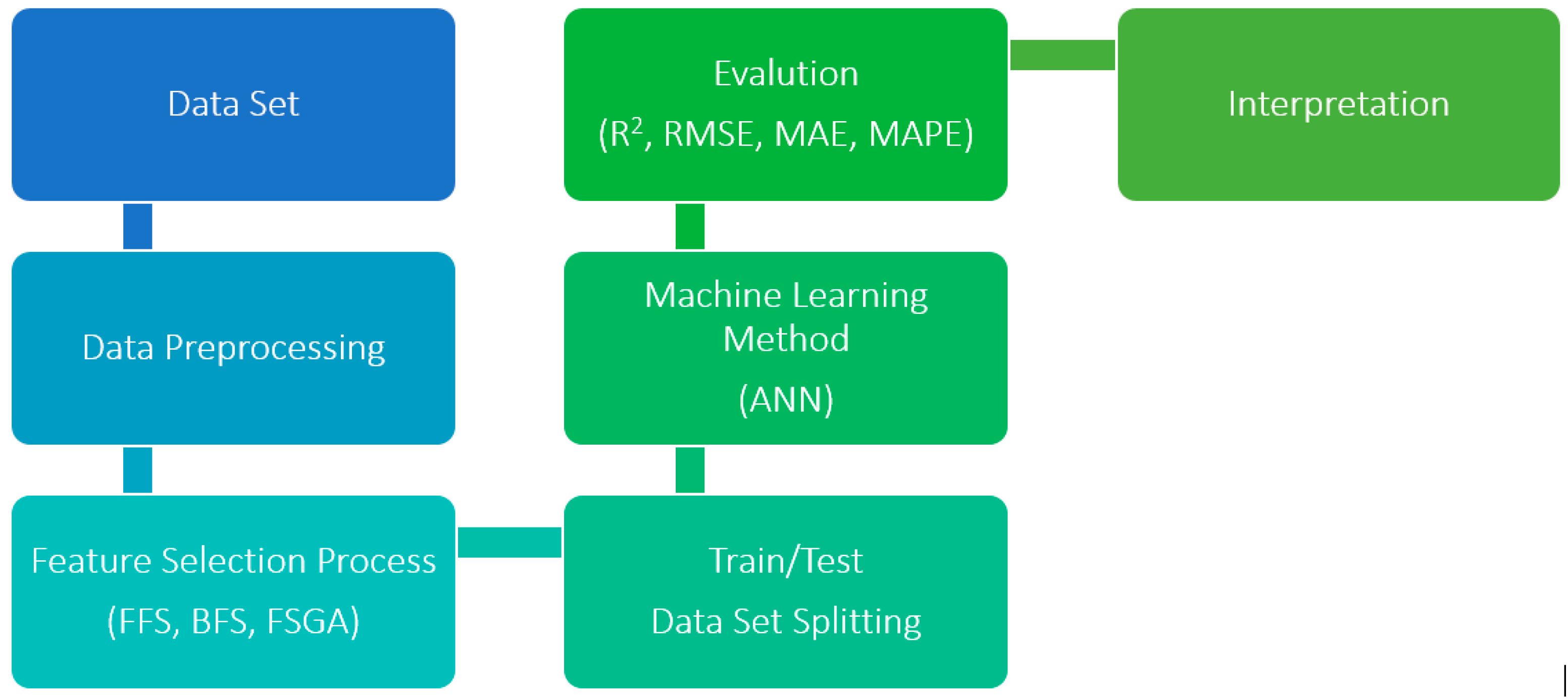
2. Materials and Methods

2.1. Tomato Characteristics Testing

The tomato variety AKT-1270 beef-type, developed by the Organic Agriculture Department of Akdeniz University Manavgat Vocational School, was utilised in this investigation (Figure 1). Using the USDA colour chart as a guide (green, breaker, changing, pink, light red, and red), the tomato fruits utilised in the studies were picked in June 2023 at the red maturity stage [44]. Out of 500 harvested tomatoes, 294 tomato fruit samples were chosen at random for analysis. They were then cleaned, dried, and kept at 20 °C until needed.

Total soluble solid (TSS)

TSS, measured in Brix, was determined using a digital refractometer (ATAGO Classic HHR-2N), and the values are presented as percentages [45].

Titratable acidity (TA) and pH

The tomato’s TA was ascertained utilising the titration process. A 10 mL sample of tomato juice was titrated against 0.1 N NaOH and the values were given as a citric acid percentage [46]. A pH meter was used to measure the pH.

Total dry matter (TDM) and Ash

Every tomato fruit sample was dried at 70 °C in an oven. Fruits were first dried at 100 °C and then burned in an oven at 525 °C after they were weighed. The ash content was expressed in percentage [47].

Tomato Fruit firmness

Two locations in the equatorial region were used to assess the tomato’s fruit firmness using a PCE-PTR 200 penetrometer (pushing probe 6 mm) [48].

Fructose and Glycose content

To ascertain the sugar content of every sample, a 50 mL Erlenmeyer flask was filled with 10 g of sample, followed by the addition of 20 mL of double-distilled water. An ultra-turrax homogeniser was used to smash the mixture, and it was centrifuged for 30 min at 20 °C at 6000 rpm. A total of 10 mL of the clear portion was taken, 10 mL of distilled water was added, and 10 mL of filter paper was used to filter it. The filtrate was filtered through a membrane filter, combined with two millilitres of acetonitrile, and subjected to HPLC analysis [49].

Lycopene content

The spectrophotometer device was used to determine the amount of lycopene present in fruits. Samples of fruit weighing 0.5 g were taken from each puree and placed into a 50 mL erlenmeyer flask along with 10 mL of hexane and 5 mL of 95% ethanol. Samples were extracted on ice for 15 min at 180 rpm using an orbital shaker. Each vial was filled with 3 mL of deionised water and shaken again, this time for five minutes while the samples remained on ice. Phase separation was then allowed to occur by leaving the vials at room temperature for five minutes. A quartz cuvette with a 1 cm path length and a hexane blank at 503 nm was used to measure the upper hexane layer’s absorbance. The absorbance at 503 nm and the sample weight were then used to estimate the lycopene concentration of each sample [50].

Vitamin C (Ascorbic acid)

Ascorbic acid was extracted from tomato fruits in accordance with Karhan et al. (2004) [51]. Five grams of sample weight and five millilitres of 6% metaphosphoric acid were added. After that, the sample was centrifuged for 10 min at 4 °C at 6500 rpm. After collecting 0.5 mL of the supernatant, 6% metaphosphoric acid was added, and the mixture was finished in a 10 mL volumetric flask. This extract was run through a membrane filter with a 0.45 µm pore size. The values obtained from the analysis were given in milligrams of ascorbic acid per gram of fresh tomato fruit.

Nutrient elements

Tomato samples’ levels of calcium (Ca), potassium (K), magnesium (Mg), phosphorus (P), and micromineral manganese (Mn) were measured in accordance with Kacar and Inal (2010) [52].

Colour properties

Peel coloiur L (brightness; 100 white, 0 black), a (+ red; − green) and b (+ yellow; − blue), hue and chroma were ascertained in the cheek area of 294 fruits with a 3NH NR100 colorimeter (Shenzhen Threenh Technology, Shenzhen, China) [53].

2.2. Linear Regression

Linear regression analysis is the process by which the predictor variables (explanatory variables) in a linear model express the predicted variable (target variable). In this method, where the relationship between variables is analysed one-way, while MLR is used when there are multiple predictor variables, simple linear regression is used when there is only one predictor variable [54]. MLR equation is expressed as follows:

$$Y_i={{\beta }_0+\beta }_1{X}_{1i}+{\beta }_2{X}_{2i}+\dots +{\beta }_k{X}_{ki}+{\epsilon }_i$$

Here, Y is the predicted variable, X_i is the predictor variable, and the error term is ε [55].

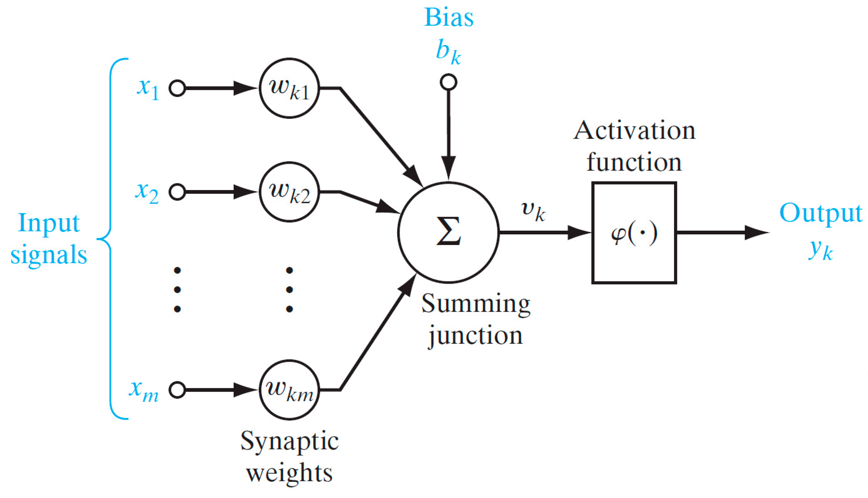
2.3. Artificial Neural Networks

The human brain is an incredibly intricate, non-linear, parallel computer (processor). It has structural components called neurons to carry out several tasks such as perception, identification of patterns, and motor control [56]. There are an estimated 1011 neurons in the brain, and these neurons are connected to each other with an estimated 1015 connections [57]. ANN can be expressed as the summary of the computational model of the brain [58]. ANNs are a subset of artificial intelligence that aims to replicate how the brain processes and stores information. It is a network structure that functions by establishing connections between neurons, which are units of mathematical processing [59]. Figure 2 shows the artificial neuron structure.

There are many definitions and approaches to ANNs, but they are distributed processors composed of neurons [58]. In ANNs, information is obtained from the network through a learning process. Connections between neurons are called synaptic weights, and they are utilised to store newly learned information [56]. In ANNs, learning takes place with the system called the backpropagation algorithm. Learning is actually a matter of determining synaptic weights. One of the supervised learning models, the ANN, uses input–output pairs as its training set. An ANN searches for a function that, given inputs, generates outputs. Applying training data repeatedly over time the network approximates a function for that input space [59].

When the studies in the literature are examined, there are different ANN models such as MLP, SOM, RBF, CNN, RNN, LSTM, LVQ, and LAM [60,61,62,63,64,65]. In this study, feed-forward ANN, which is the most preferred and frequently used in the literature, was used.

In the MLR analysis, the predictor variables specified in Figure 2 were included in the analysis. However, in order for the model established in MLR analysis to be reliable and usable, it must pass multicollinearity, heteroscedasticity, linearity, and normality diagnostic tests [55]. High correlation leads to a multicollinearity problem. To detect this problem, the VIF value among the predictor variables must be examined. A VIF < 10 indicates that there is no multicollinearity in the model [66]. As each VIF value is lower than 10 (all VIFs < 10), the model does not have a multicollinearity issue. For heteroskedasticity detection, Breusch–Pagan/Cook–Weiseberg heteroskedasticity detection was performed [67]. The result is p > 0.05. According to this result, there is no heteroscedasticity in the model. To determine linearity, the Augmented Component Plus Residual graph of the predictor variables in the model was drawn [55]. It was observed that the predictor variables were linearly related to the predicted variable. One of the most important steps of MLR is that the errors of the estimated model come from a population that is normally distributed. We performed a Shapiro–Wilk W test to check whether the errors were normally distributed or not [54]. Since the result is p > 0.05, there is no normality problem in the model. Figure 3 displays this study’s flow chart.

ML is actually a step in the process of discovering the information contained in databases. Different methodologies such as SEMMA, CRISP-DM, and KDD are followed when discovering knowledge from data. Every methodology’s aim is to reveal the information that is hidden in the data. Many steps are similar and common in these methodologies, one of which is the ML stage. Following the purpose of our study, the steps shown in Figure 3 were processed sequentially. As a first step, data that were suitable for our purpose were selected from the data in the database. Secondly, the data preprocessing phase was started. At this stage, descriptive statistics of the data included in the analysis were examined. At this stage, it was also checked whether there was any missing data in the data set, and the presence of outliers was investigated with extreme value analysis. In the third stage, feature selection methods with forward, backwards, and genetic algorithms were applied to determine the presence of effective and ineffective variables in predicting the target variable. Once these phases are finished, the data set is split into two partitions, known as training (70%) and testing (30%) partitions in the ML literature. The fourth stage of the knowledge discovery process is the modeling stage where ML methods are applied. Here, the ANN method was applied. The next stage is the evaluation stage, where the metrics used to evaluate the established models are obtained. Since the selection of evaluation criteria and visualisation instruments is made, the evaluation phase is considerable. Choosing the correct evaluation criteria and visualisation instruments is important for the correct interpretation of the models. At this stage, the metrics R², MAE, MAPE, and RMSE, which are widely employed in the assessment of regression problems [68,69], were calculated. In the final stage, the models are interpreted. Formulations of metrics that used in this study are shown in Equations (1)–(4) $Y_i-{\widehat{Y}}_i$.

$$RMSE=\sqrt{{\displaystyle \frac{1}{m}}{\sum }_{i=1}^m{\left(X_i-Y_i\right)}^2},$$

(1)

$$MAE={\displaystyle \frac{1}{m}}{\sum }_{i=1}^m\left|X_i-Y_i\right|,$$

(2)

$$MAPE={\displaystyle \frac{1}{m}}{\sum }_{i=1}^m\left|{\displaystyle \frac{Y_i-X_i}{Y_i}}\right|,$$

(3)

$$R^2=1-{\displaystyle \frac{{\sum }_{i=1}^m{\left(X_i-Y_i\right)}^2}{{\sum }_{i=1}^m{\left(\overline{Y}-Y_i\right)}^2}},$$

(4)

Defined as the arithmetic mean of the absolute error (e), MAE is a criterion used in the assessment of the regression models. It takes values ranging between [0, ∞); the model’s MAE value close to zero indicates that the regression model is accomplished [70]. Another metric is RMSE, which is frequently used in evaluating the regression problem and is sensitive to outliers. The square root of the sum of the error squares’ arithmetic mean is used to compute RMSE. It can take values between [0, ∞). Both RMSE and MAE metrics are measured in the same unit as the target value [71]. It takes values between [0, ∞), and the model’s RMSE value close to zero points out that the regression model is accomplished [72]. MAPE is another statistical value that is commonly employed in assessing regression problems like MAE and RMSE. It shows the percentage deviation of the predicted variable from its actual value. While it takes values between [0, ∞), as in both RMSE and MAE, the regression model is accomplished when the value is near zero [73]. The coefficient of determination, or simply R², is a measure of goodness of fit and is defined as the explained variance in the predicted variable. The remaining ratio, (1–R²), is the variance not predicted by the model. The R² metric can take values between [0, 1], and, if it takes the value 1, the predictor variables are interpreted as fully explaining the predicted variable. Otherwise, predictor variables fail to explain the predicted variable. To summarise, the greater the accuracy of a model in making estimations, the closer its R² will be to 1 [74].

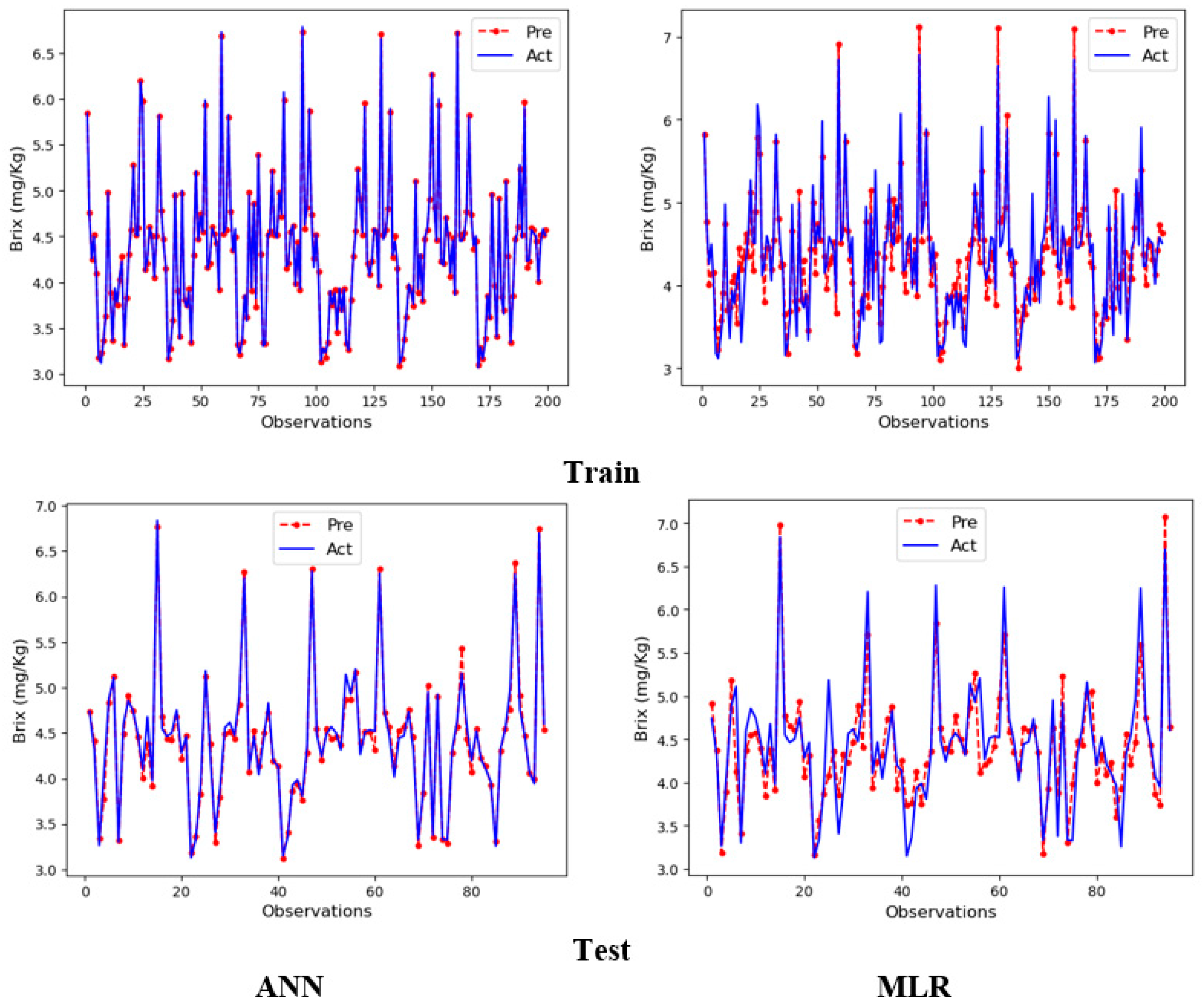
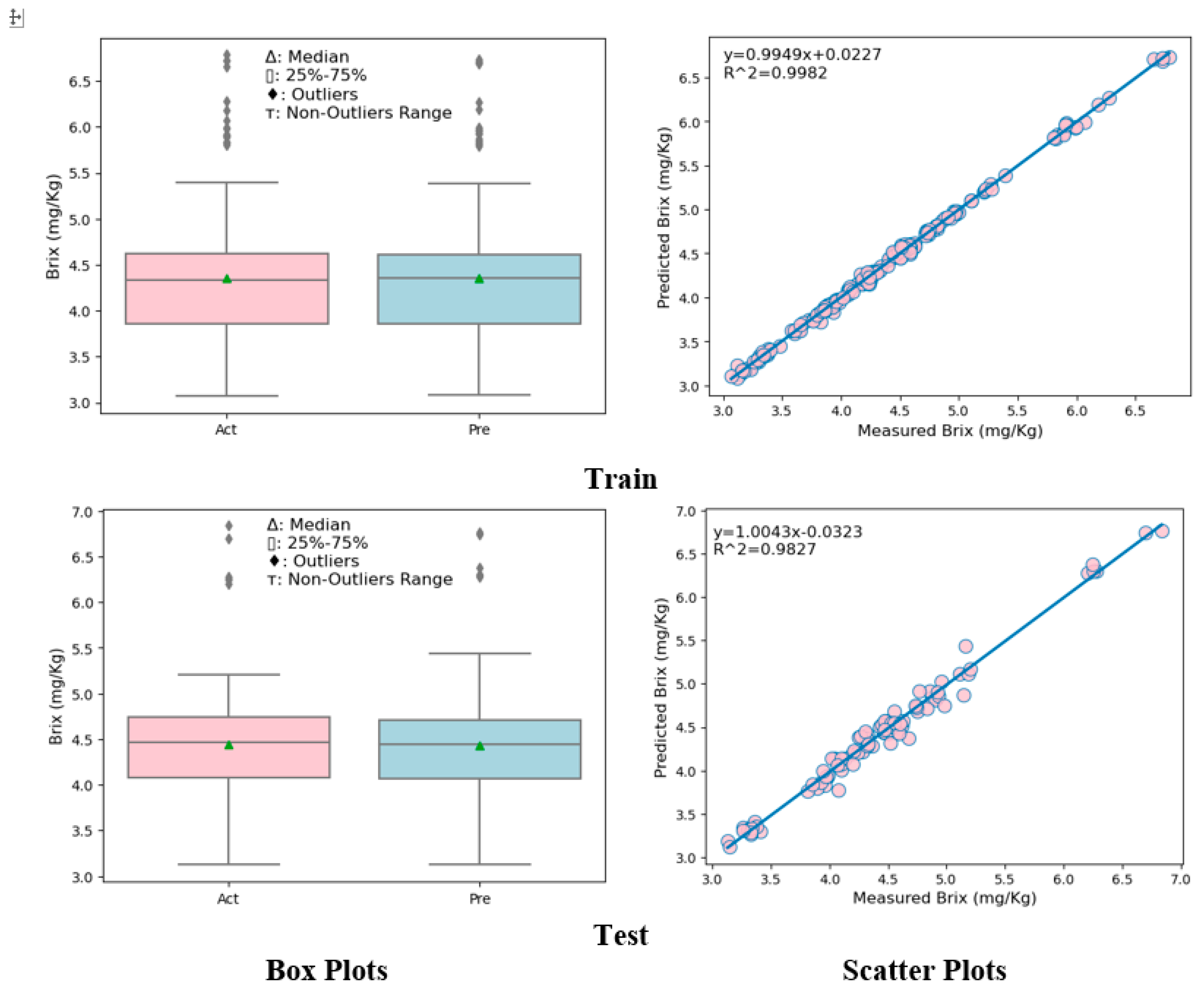
3. Results and Discussion

A descriptive statistical analysis of the values obtained as a result of the trials conducted on the tomato fruits used in this study can be found in

Table 1. Descriptive statistics of the variables ¹.

Variables	Mean	Min	Max	Std,Dev	Variables	Mean	Min	Max	Std,Dev
Brix *	4.32	2.90	6.82	0.76	a	24.78	16.99	31.78	3.07
TKM	5.72	4.14	9.15	0.84	b	23.30	18.55	31.97	3.01
Ash	0.50	0.30	0.75	0.09	C	34.06	25.27	45.02	3.92
pH	4.25	4.03	4.46	0.10	h	43.48	35.43	49.97	3.11
Acidity	0.38	0.27	0.54	0.06	Manganese	1.13	0.69	1.76	0.22
Hardness	1.07	0.55	1.70	0.26	Sodium	32.35	22.68	42.85	4.95
Fructose	1.24	0.51	2.18	0.29	Calcium	360.62	206.56	583.91	87.62
Glucose	1.10	0.48	2.05	0.31	Potassium	2305.29	1305.35	2936.53	365.29
Lycopene	51.32	20.08	105.23	15.72	Magnesium	115.41	78.32	171.63	23.58
Vitamin C	20.45	12.98	29.54	3.69	Phosphor	169.65	99.39	325.63	38.16
L	40.07	35.70	46.16	2.10

¹ Number of observations: 294, * Target Variable.

.

Table 2. Results of the MLR.

Variables	Std.	Beta	Std.	p Value
TKM	0.588	0.047	11.356	0.000
Acidity	0.267	0.592	6.238	0.000
Vitamin C	0.061	0.008	−1.72	0.087
L	0.213	0.017	−4.637	0.000
a	1.557	0.153	2.665	0.008
b	2.814	0.152	4.986	0.000
C	3.828	0.188	−4.239	0.000
h	0.585	0.062	−2.386	0.018
Potassium (K)	0.216	0.000	−3.934	0.000
Magnesium (Mg)	0.116	0.002	2.084	0.038
Sodium (Na)	0.199	0.007	−4.55	0.000
Phosphor (P)	0.217	0.001	3.552	0.000
Constant	2.816	9.79	3.476	0.001

displays the MLR model’s results established to estimate the amount of brix in tomato fruit.

According to the MLR model, while TKM, acidity, Vitamin C, L, a, b, C, h, K, Mg, Na, and P are significant, ash, pH, hardness, fructose, glucose, Ca, Mn, and lycopene are insignificant. All variables are significant at the 0.05 error level, except Vitamin C (significant at the 0.10 error level). According to the MLR result, the regression equation is given in Equation (5).

$$\begin{gathered} \widehat{brix}=2.816+0.588TKM+0.267Acidity-0.061vitC-0.213L+1.557a+ \\ 2.814b-3.828C-0.585-0.216K+0.116Mg-0.199Na+0.217P \end{gathered}$$

(5)

Table 3. Metric results of the MLR and ANN.

Technique	Evaluation Metrics	Training Partition	Testing Partition
MLR	MAE	0.2349	0.2573
	RMSE	0.3048	0.3343
	R2	0.8441	0.7843
	MAPE	5.5368	5.8199
ANN	MAE	0.0250	0.0720
	RMSE	0.0331	0.0964
	R2	0.9982	0.9827
	MAPE	0.5814	1.6240

displays the outcomes of the MLR and ANN models. According to the training data set results of the MLR model established to estimate the amount of brix in tomato fruit, the results can be calculated as MAE: 0.2349, RMSE: 0.3048, R²: 0.8441, and MAPE: 5.5368, while, according to the ANN model, MAE: 0.0250, RMSE: 0.031, R²: 0.9982, and MAPE: 0.5814.

As seen in Table 3, the training and test data results of the MLR model are close to each other. A similar situation applies to the ANN model. Accordingly, there is no overlearning problem in MLR and ANN models. As seen in Table 1, the training and test data results of the MLR model are close to each other. A similar situation applies to the ANN model. Accordingly, there is no overlearning problem in MLR and ANN models. Based on the test data set findings, the MLR model predicts the amount of Brix with an average error of 0.2573, while the ANN model estimates it with an error of 0.0250. According to the RMSE result of the MLR model, the model estimates the brix amount with an RMSE error of 0.3343, while the ANN model estimates it with an RMSE error of 0.031. In the MLR model, the explained variation is approximately 78%, while, in the ANN model, it is 99.8%. The MAPE value of MLR is 5.8199, the predicted variable, namely, the brix amount, can be predicted with an error of approximately 5.8%, while the ANN model makes a prediction with an error of approximately 0.6%. However, in light of these outcomes, it is seen that the ANN model is more successful and makes better predictions than the MLR model in the training data set. These comments can also be made for the training dataset. Figure 4 shows line plots created with data from the ANN and MLR model results.

While the plots in the upper part are created with the data obtained from the training results of the models, the plots in the lower part are created with the data obtained from the test results of the models. Figure 4 illustrates how successful the models created using both ANN and MLR techniques are on the whole in the training set. The lines of both real and estimated values overlap in the plots. On the other hand, in the training partition, it is clearly seen in the plots that the ANN method is more successful than the MLR method, and the metric results also support the plots. It can be concluded that the ANN model outperforms the MLR model in the testing partition. As this situation can be clearly seen in the plots at the bottom of Figure 4, the metric results also support these plots. The box plots and scatter plots for the ANN model’s training and testing partitions are displayed in Figure 5.

In recent years, many researchers have been using ML techniques to solve problems in many branches of agricultural science. ML methods are more advantageous compared to traditional statistical techniques such as MLR in solving nonlinear complex problems [33,75,76,77]. Although ML methods are very diverse, the ANN method is preferred in most studies, especially to estimate the amount of solid content in fruits and vegetables, while MLR, one of the traditional statistical methods, is preferred as a comparison. In the study of Huang et al., the amount of soluble solids in loquat fruit was estimated by ANN and MLR. In this study, while, in the ANN model (both in the training and test data sets), MAE and RMSE were lower than in the MLR model, R² was greater. In the test data set, the R² value of the ANN model is 0.84, while it is 0.64 in the MLR model. The MAE value of the ANN model is 0.138, while it is 0.149 in the MLR model. The RMSE value of the ANN model is 0.177, while it is 0.181 in the MLR model. In this study, while better R² values were obtained in both ANN and MLR models compared to Huang et al.‘s study, MAE and RMSE results were close to each other. In the study of Torkashvand et al., like that previous study, the ANN model outperforms MLR in all metrics. Many studies have reported that ANN model results are better than MLR model results. Accordingly, it can be said that ML models give better results than classical methods [31,34,78,79,80].

The box plots and scatter plots for the MLR model’s training and testing partitions are displayed in Figure 6.

In this study, the ANN model was more successful in predicting better results than the MLR model. When comparing the ANN model with the MLR model in predicting the amount of brix, MAE, RMSE and MAPE decreased by 89%, while R² increased by 18% in the training data set. When the ANN model was matched with the MLR model in predicting the amount of brix, MAE and MAPE decreased by 72%, RMSE decreased by 71%, and R² increased by 25% in the testing data set. Together with these details, graphs are used to visually represent and compare the expected and actual values of the ANN and MLR models during the training and testing phases (Figure 5 and Figure 6).

4. Conclusions

The prediction of the total soluble solid (TSS) content in tomatoes has important implications for various stakeholders in the agricultural and food industries. Tomato producers can benefit from optimising harvest time, improving quality control, and predicting yield in advance. The food processing industry can enhance product development, quality assurance, and process optimisation. Consumers can make informed choices based on accurate product information. Researchers can deepen their understanding of tomato ripening, develop new varieties, and improve predictive models. This study’s results provide a rapid and precise method for estimating TSS, contributing to increased efficiency, sustainability, and consumer satisfaction within the tomato industry.

In this study, we estimate the amount of brix (soluble solids) in beef tomato fruit by ANN and MLR methods. To evaluate the models R², MAE, MAPE, and RMSE metrics were used. The regression equation is written according to the coefficients obtained as a result of MLR analysis. According to the MLR model, while TKM, acidity, Vitamin C, L, a, b, C, h, K, Mg, Na, and P are significant, ash, pH, hardness, fructose, glucose, Ca, Mn, and lycopene are insignificant. All variables are significant at the 0.05 error level, except Vitamin C (significant at the 0.10 error level). Based on the metric outcomes that were acquired, the ANN model was more successful in both the training and testing partitions. Line plots created for training and testing splits also support the metric results. Furthermore, graphs have been used to visually represent and compare the actual and predicted values of the models in each of the two partitions. According to the training data set results of the MLR model established to estimate the amount of brix in tomato fruit, the results were calculated as MAE: 0.2349, RMSE: 0.3048, R²: 0.8441 and MAPE: 5.5368, while, according to the ANN model, they were calculated as MAE: 0.0250, RMSE: 0.031, R²: 0.9982 and MAPE: 0.5814. Since the training and testing results of both ANN and MLR models are close to each other, it can be said that the models are consistent and there is no overlearning problem in the models.

References

1. FAO FAOSTAT. Available online: https://www.fao.org/faostat/en/#data/QCL (accessed on 28 January 2024).
2. Abdel-Sattar, M.; Al-Saif, A.M.; Aboukarima, A.M.; Eshra, D.H.; Sas-Paszt, L. Quality Attributes Prediction of Flame Seedless Grape Clusters Based on Nutritional Status Employing Multiple Linear Regression Technique. Agriculture 2022, 12, 1303. [Google Scholar] [CrossRef]
3. Olaniyi, J.O.; Akanbi, W.B.; Adejumo, T.A.; Akande, O.G. Growth, Fruit Yield and Nutritional Quality of Tomato Varieties. African J. Food Sci. 2010, 4, 398–402. [Google Scholar]
4. Quinet, M.; Angosto, T.; Yuste-Lisbona, F.J.; Blanchard-Gros, R.; Bigot, S.; Martinez, J.P.; Lutts, S. Tomato Fruit Development and Metabolism. Front. Plant Sci. 2019, 10, 475784. [Google Scholar] [CrossRef]
5. Tieman, D.M.; Zeigler, M.; Schmelz, E.A.; Taylor, M.G.; Bliss, P.; Kirst, M.; Klee, H.J. Identification of Loci Affecting Flavour Volatile Emissions in Tomato Fruits. J. Exp. Bot. 2006, 57, 887–896. [Google Scholar] [CrossRef] [PubMed]
6. Beckles, D.M.; Hong, N.; Stamova, L.; Luengwilai, K. Biochemical Factors Contributing to Tomato Fruit Sugar Content: A Review. Fruits 2012, 67, 49–64. [Google Scholar] [CrossRef]
7. Li, N.; Wang, J.; Wang, B.; Huang, S.; Hu, J.; Yang, T.; Asmutola, P.; Lan, H.; Qinghui, Y. Identification of the Carbohydrate and Organic Acid Metabolism Genes Responsible for Brix in Tomato Fruit by Transcriptome and Metabolome Analysis. Front. Genet. 2021, 12, 714942. [Google Scholar] [CrossRef] [PubMed]
8. Bergougnoux, V. The History of Tomato: From Domestication to Biopharming. Biotechnol. Adv. 2014, 32, 170–189. [Google Scholar] [CrossRef]
9. Georgelis, N. High Fruit Sugar Characterization, Inheritance and Linkage of Molecular Markers in Tomato; University of Florida: Gainesville, FL, USA, 2002. [Google Scholar]
10. Tieman, D.; Zhu, G.; Resende, M.F.R.; Lin, T.; Nguyen, C.; Bies, D.; Rambla, J.L.; Beltran, K.S.O.; Taylor, M.; Zhang, B.; et al. A Chemical Genetic Roadmap to Improved Tomato Flavor. Science 2017, 355, 391–394. [Google Scholar] [CrossRef]
11. Ikeda, H.; Hiraga, M.; Shirasawa, K.; Nishiyama, M.; Kanahama, K.; Kanayama, Y. Analysis of a Tomato Introgression Line, IL8-3, with Increased Brix Content. Sci. Hortic. 2013, 153, 103–108. [Google Scholar] [CrossRef]
12. Amr, A.; Raie, W.Y. Tomato Components and Quality Parameters. A Review. Jordan J. Agric. Sci. 2022, 18, 199–220. [Google Scholar] [CrossRef]
13. de Brito, A.A.; Campos, F.; dos Nascimento, A.R.; de Carvalho Corrêa, G.; de Silva, F.A.; de Almeida Teixeira, G.; Júnior, L.C.C. Determination of Soluble Solid Content in Market Tomatoes Using Near-Infrared Spectroscopy. Food Control 2021, 126, 108068. [Google Scholar] [CrossRef]
14. Kabas, O.; Kayakus, M.; Ünal, İ.; Moiceanu, G. Deformation Energy Estimation of Cherry Tomato Based on Some Engineering Parameters Using Machine-Learning Algorithms. Appl. Sci. 2023, 13, 8906. [Google Scholar] [CrossRef]
15. Maulud, D.H.; Mohsin Abdulazeez, A. A Review on Linear Regression Comprehensive in Machine Learning. J. Appl. Sci. Technol. Trends 2020, 1, 140–147. [Google Scholar] [CrossRef]
16. Belouz, K.; Nourani, A.; Zereg, S.; Bencheikh, A. Prediction of Greenhouse Tomato Yield Using Artificial Neural Networks Combined with Sensitivity Analysis. Sci. Hortic. 2022, 293, 110666. [Google Scholar] [CrossRef]
17. Tripathi, P.; Kumar, N.; Rai, M.; Shukla, P.K.; Verma, K.N. Applications of Machine Learning in Agriculture. In Smart Village Infrastructure and Sustainable Rural Communities; Khan, M., Gupta, B., Verma, A., Praveen, P., Peoples, C., Eds.; IGI Global: Hershey, PA, USA, 2023; pp. 99–118. [Google Scholar]
18. Attri, I.; Awasthi, L.K.; Sharma, T.P. Machine Learning in Agriculture: A Review of Crop Management Applications. Multimed. Tools Appl. 2024, 83, 12875–12915. [Google Scholar] [CrossRef]
19. Araújo, S.O.; Peres, R.S.; Ramalho, J.C.; Lidon, F.; Barata, J. Machine Learning Applications in Agriculture: Current Trends, Challenges, and Future Perspectives. Agronomy 2023, 13, 2976. [Google Scholar] [CrossRef]
20. Yang, B.; Gao, Y.; Yan, Q.; Qi, L.; Zhu, Y.; Wang, B. Estimation Method of Soluble Solid Content in Peach Based on Deep Features of Hyperspectral Imagery. Sensors 2020, 20, 5021. [Google Scholar] [CrossRef]
21. Akbarzadeh, S.; Paap, A.; Ahderom, S.; Apopei, B.; Alameh, K. Plant Discrimination by Support Vector Machine Classifier Based on Spectral Reflectance. Comput. Electron. Agric. 2018, 148, 250–258. [Google Scholar] [CrossRef]
22. Son, N.T.; Chen, C.F.; Chen, C.R.; Guo, H.Y.; Cheng, Y.S.; Chen, S.L.; Lin, H.S.; Chen, S.H. Machine Learning Approaches for Rice Crop Yield Predictions Using Time-Series Satellite Data in Taiwan. Int. J. Remote Sens. 2020, 41, 7868–7888. [Google Scholar] [CrossRef]
23. Shah, S.S.A.; Zeb, A.; Qureshi, W.S.; Malik, A.U.; Tiwana, M.; Walsh, K.; Amin, M.; Alasmary, W.; Alanazi, E. Mango Maturity Classification Instead of Maturity Index Estimation: A New Approach towards Handheld NIR Spectroscopy. Infrared Phys. Technol. 2021, 115, 103639. [Google Scholar] [CrossRef]
24. Zhao, C.; Lee, W.S.; He, D. Immature Green Citrus Detection Based on Colour Feature and Sum of Absolute Transformed Difference (SATD) Using Colour Images in the Citrus Grove. Comput. Electron. Agric. 2016, 124, 243–253. [Google Scholar] [CrossRef]
25. Ozaktan, H.; Çetin, N.; Uzun, S.; Uzun, O.; Ciftci, C.Y. Prediction of Mass and Discrimination of Common Bean by Machine Learning Approaches. Environ. Dev. Sustain. 2024, 26, 18139–18160. [Google Scholar] [CrossRef]
26. Kour, V.P.; Arora, S. Fruit Disease Detection Using Rule-Based Classification. Adv. Intell. Syst. Comput. 2019, 851, 295–312. [Google Scholar] [CrossRef]
27. Liu, B.; Zhang, Y.; He, D.J.; Li, Y. Identification of Apple Leaf Diseases Based on Deep Convolutional Neural Networks. Symmetry 2017, 10, 11. [Google Scholar] [CrossRef]
28. Castro, W.; Oblitas, J.; De-La-Torre, M.; Cotrina, C.; Bazan, K.; Avila-George, H. Classification of Cape Gooseberry Fruit According to Its Level of Ripeness Using Machine Learning Techniques and Different Color Spaces. IEEE Access 2019, 7, 27389–27400. [Google Scholar] [CrossRef]
29. Emamgholizadeh, S.; Parsaeian, M.; Baradaran, M. Seed Yield Prediction of Sesame Using Artificial Neural Network. Eur. J. Agron. 2015, 68, 89–96. [Google Scholar] [CrossRef]
30. Tang, C.; He, H.; Li, E.; Li, H. Multispectral Imaging for Predicting Sugar Content of ‘Fuji’ Apples. Opt. Laser Technol. 2018, 106, 280–285. [Google Scholar] [CrossRef]
31. Huang, X.; Wang, H.; Luo, W.; Xue, S.; Hayat, F.; Gao, Z. Prediction of Loquat Soluble Solids and Titratable Acid Content Using Fruit Mineral Elements by Artificial Neural Network and Multiple Linear Regression. Sci. Hortic. 2021, 278, 109873. [Google Scholar] [CrossRef]
32. Özreçberoğlu, N.; Kahramanoğlu, İ. Mathematical Models for the Estimation of Leaf Chlorophyll Content Based on RGB Colours of Contact Imaging with Smartphones: A Pomegranate Example. Folia Hortic. 2020, 32, 57–67. [Google Scholar] [CrossRef]
33. Abdipour, M.; Ramazani, S.H.R.; Younessi-Hmazekhanlu, M.; Niazian, M. Modeling Oil Content of Sesame (Sesamum Indicum L.) Using Artificial Neural Network and Multiple Linear Regression Approaches. J. Am. Oil Chem. Soc. 2018, 95, 283–297. [Google Scholar] [CrossRef]
34. Torkashvand, A.M.; Ahmadi, A.; Nikravesh, N.L. Prediction of Kiwifruit Firmness Using Fruit Mineral Nutrient Concentration by Artificial Neural Network (ANN) and Multiple Linear Regressions (MLR). J. Integr. Agric. 2017, 16, 1634–1644. [Google Scholar] [CrossRef]
35. Pflanz, M.; Zude, M. Spectrophotometric Analyses of Chlorophyll and Single Carotenoids during Fruit Development of Tomato (Solanum Lycopersicum L.) by Means of Iterative Multiple Linear Regression Analysis. Appl. Opt. 2008, 47, 5961–5970. [Google Scholar] [CrossRef] [PubMed]
36. Vursavuş, K.; Kesilmiş, Z.; Benal, Y.; Ondokuz, Y.; Üniversitesi, M.; Vursavus, K.K.; Kesilmis, Z.; Oztekin, Y.B. Nondestructive Dropped Fruit Impact Test for Assessing Tomato Firmness. Chem. Eng. Trans. 2017, 58, 1–6. [Google Scholar] [CrossRef]
37. Takahashi, N.; Yokoyama, N.; Takayama, K.; Nishina, H. Estimation of Tomato Fruit Lycopene Content after Storage at Different Storage Temperatures and Durations. Environ. Control Biol. 2018, 56, 157–160. [Google Scholar] [CrossRef]
38. Garcia, M.B.; Ambat, S.; Adao, R.T. Tomayto, Tomahto: A Machine Learning Approach for Tomato Ripening Stage Identification Using Pixel-Based Color Image Classification. In Proceedings of the 2019 IEEE 1th International Conference on Humanoid, Nanotechnology, Information Technology, Communication and Control, Environment, and Management, HNICEM, Laoang, Philippines, 29 November–1 December 2019. [Google Scholar] [CrossRef]
39. Berrueta, C.; Heuvelink, E.; Giménez, G.; Dogliotti, S. Estimation of Tomato Yield Gaps for Greenhouse in Uruguay. Sci. Hortic. 2020, 265, 109250. [Google Scholar] [CrossRef]
40. Nyalala, I.; Okinda, C.; Chao, Q.; Mecha, P.; Korohou, T.; Yi, Z.; Nyalala, S.; Jiayu, Z.; Chao, L.; Kunjie, C. Weight and Volume Estimation of Single and Occluded Tomatoes Using Machine Vision. Int. J. Food Prop. 2021, 24, 818–832. [Google Scholar] [CrossRef]
41. Pathare, P.B.; Al-Dairi, M. Bruise Damage and Quality Changes in Impact-Bruised, Stored Tomatoes. Horticulturae 2021, 7, 113. [Google Scholar] [CrossRef]
42. Égei, M.; Takács, S.; Palotás, G.; Palotás, G.; Szuvandzsiev, P.; Daood, H.G.; Helyes, L.; Pék, Z. Prediction of Soluble Solids and Lycopene Content of Processing Tomato Cultivars by Vis-NIR Spectroscopy. Front. Nutr. 2022, 9, 845317. [Google Scholar] [CrossRef]
43. Dhakshina Kumar, S.; Esakkirajan, S.; Vimalraj, C.; Keerthi Veena, B. Design of Disease Prediction Method Based on Whale Optimization Employed Artificial Neural Network in Tomato Fruits. Mater. Today Proc. 2020, 33, 4907–4918. [Google Scholar] [CrossRef]
44. USDA. U.S. Standards for Grades of Fresh Tomatoes; USDA: Washington, DC, USA, 1991.
45. Javanmardi, J.; Kubota, C. Variation of Lycopene, Antioxidant Activity, Total Soluble Solids and Weight Loss of Tomato during Postharvest Storage. Postharvest Biol. Technol. 2006, 41, 151–155. [Google Scholar] [CrossRef]
46. Cemeroğlu, B. Meyve ve Sebze İşleme Endüstrisinde Temel Analiz Metotları; Biltav Yayınları: Ankara, Turkey, 1992. [Google Scholar]
47. Gıda İşleri Genel Müdürlüğü. Gıda Maddeleri Muayene ve Analiz Yöntemleri; T.C. Tarım Orman ve Köy İşleri Bakanlığı Gıda İşleri Genel Müdürlüğü: Ankara, Turkey, 1983.
48. Uluisik, S.; Oney-Birol, S. Uncovering Candidate Genes Involved in Postharvest Ripening of Tomato Using the Solanum Pennellii Introgression Line Population by Integrating Phenotypic Data, RNA-Seq, and SNP Analyses. Sci. Hortic. 2021, 288, 110321. [Google Scholar] [CrossRef]
49. Topuz, A. Determination of Some Physical, Chemical Properties of Loquat Cultivars (Eriobotrya Japonica L.) and Possibilities of Their Being Processed into Marmalade, Nectar and Canned Fruit. Master’s Thesis, Akdeniz University, Antalya, Turkey, 1998. [Google Scholar]
50. Fish, W.W.; Perkins-Veazie, P.; Collins, J.K. A Quantitative Assay for Lycopene That Utilizes Reduced Volumes of Organic Solvents. J. Food Compos. Anal. 2002, 15, 309–317. [Google Scholar] [CrossRef]
51. Karhan, M.; Aksu, M.; Tetik, N.; Turhan, I. Kinetic Modeling of Anaerobic Thermal Degradation of Ascorbic Acid In Rose Hip (Rosa Canina L.) Pulp. J. Food Qual. 2004, 27, 311–319. [Google Scholar] [CrossRef]
52. Kacar, B.; İnal, A. Bitki Analizleri; Nobel Yayın: Ankara, Turkey, 2010; ISBN 978-605-395-036-3. [Google Scholar]
53. Kaymak, H.Ç.; Rastilantie, M.; Caglar Kaymak, H.; Ozturk, I.; Kalkan, F.; Kara, M.; Ercisli, S. Color and Physical Properties of Two Common Tomato (Lycopersicon Esculentum Mill.) Cultivars. Agric. Environ. 2010, 8, 44–46. [Google Scholar]
54. Mert, M. SPSS/STATA Yatay Kesit Veri Analizi Bilgisayar Uygulamaları; Detay Yayıncılık: Ankara, Turkey, 2016. [Google Scholar]
55. Su, X.; Yan, X.; Tsai, C.L. Linear Regression. Wiley Interdiscip. Rev. Comput. Stat. 2012, 4, 275–294. [Google Scholar] [CrossRef]
56. Haykin, S. Neural Networks and Learning Machines, 3rd ed.; Pearson Education, Inc.: Upper Saddle River, NJ, USA, 2009. [Google Scholar]
57. Larose, D.T. Discovering Knowledge in Data: An Introduction to Data Mining; John Wiley & Sons, Inc.: Hoboken, NJ, USA, 2005. [Google Scholar]
58. Kantardzic, M. Data Mining: Concepts, Models, Methods, and Algorithms, 3rd ed.; John Wiley & Sons, Inc.: Hoboken, NJ, USA, 2019. [Google Scholar]
59. Skias, S.T. Background of the Verification and Validation of Neural Networks. In Methods and Procedures for the Verification and Validation of Artificial Neural Networks; Taylor, B.J., Ed.; Springer: NewYork, NY, USA, 2006; pp. 1–12. ISBN 0387282882. [Google Scholar]
60. Srinivasulu, S.; Jain, A. A Comparative Analysis of Training Methods for Artificial Neural Network Rainfall–Runoff Models. Appl. Soft Comput. 2006, 6, 295–306. [Google Scholar] [CrossRef]
61. Tino, P.; Benuskova, L.; Sperduti, A. Artificial Neural Network Models. In Springer Handbook of Computational Intelligence; Springer: New York, NY, USA, 2015; pp. 455–471. [Google Scholar] [CrossRef]
62. Benardos, P.G.; Vosniakos, G.C. Optimizing Feedforward Artificial Neural Network Architecture. Eng. Appl. Artif. Intell. 2007, 20, 365–382. [Google Scholar] [CrossRef]
63. Hossain, M.S.; Mahmood, H. Short-Term Photovoltaic Power Forecasting Using an LSTM Neural Network and Synthetic Weather Forecast. IEEE Access 2020, 8, 172524–172533. [Google Scholar] [CrossRef]
64. Song, X.H.; Hopke, P.K. Kohonen Neural Network as a Pattern Recognition Method Based on the Weight Interpretation. Anal. Chim. Acta 1996, 334, 57–66. [Google Scholar] [CrossRef]
65. Hernandez, L.; Baladron, C.; Aguiar, J.M.; Carro, B.; Sanchez-Esguevillas, A.J.; Lloret, J.; Massana, J. A Survey on Electric Power Demand Forecasting: Future Trends in Smart Grids, Microgrids and Smart Buildings. IEEE Commun. Surv. Tutor. 2014, 16, 1460–1495. [Google Scholar] [CrossRef]
66. García, C.; Gómez, R.S.; García, C.B. Choice of the Ridge Factor from the Correlation Matrix Determinant. J. Stat. Comput. Simul. 2019, 89, 211–231. [Google Scholar] [CrossRef]
67. Eldomiaty, T.; Eid, N.; Taman, F.; Rashwan, M. An Assessment of the Benefits of Optimizing Working Capital and Profitability: Perspectives from DJIA30 and NASDAQ100. J. Risk Financ. Manag. 2023, 16, 274. [Google Scholar] [CrossRef]
68. Aksoy, E.; Kocer, A.; Yilmaz, İ.; Akçal, A.N.; Akpinar, K. Assessing Fire Risk in Wildland–Urban Interface Regions Using a Machine Learning Method and GIS Data: The Example of Istanbul’s European Side. Fire 2023, 6, 408. [Google Scholar] [CrossRef]
69. Ercan, U.; Kocer, A. Prediction of Solar Irradiance with Machine Learning Methods Using Satellite Data. Int. J. Green Energy 2024, 21, 1174–1183. [Google Scholar] [CrossRef]
70. Duman, S.; Elewi, A.; Yetgin, Z. Distance Estimation from a Monocular Camera Using Face and Body Features. Arab. J. Sci. Eng. 2022, 47, 1547–1557. [Google Scholar] [CrossRef]
71. Hodson, T.O. Root-Mean-Square Error (RMSE) or Mean Absolute Error (MAE): When to Use Them or Not. Geosci. Model Dev. 2022, 15, 5481–5487. [Google Scholar] [CrossRef]
72. Kocer, A. Numerical Investigation of Heat Transfer and Thermo-Hydraulic Performance of Solar Air Heater with Different Ribs and Their Machine Learning-Based Prediction. J. Brazilian Soc. Mech. Sci. Eng. 2024, 46, 73. [Google Scholar] [CrossRef]
73. Chicco, D.; Warrens, M.J.; Jurman, G. The Coefficient of Determination R-Squared Is More Informative than SMAPE, MAE, MAPE, MSE and RMSE in Regression Analysis Evaluation. PeerJ Comput. Sci. 2021, 7, e623. [Google Scholar] [CrossRef] [PubMed]
74. Jierula, A.; Wang, S.; Oh, T.M.; Wang, P. Study on Accuracy Metrics for Evaluating the Predictions of Damage Locations in Deep Piles Using Artificial Neural Networks with Acoustic Emission Data. Appl. Sci. 2021, 11, 2314. [Google Scholar] [CrossRef]
75. Cortina, P.R.; Santiago, A.N.; Sance, M.M.; Peralta, I.E.; Carrari, F.; Asis, R. Neuronal Network Analyses Reveal Novel Associations between Volatile Organic Compounds and Sensory Properties of Tomato Fruits. Metabolomics 2018, 14, 1–15. [Google Scholar] [CrossRef]
76. Lan, H.; Wang, Z.; Niu, H.; Zhang, H.; Zhang, Y.; Tang, Y.; Liu, Y. A Nondestructive Testing Method for Soluble Solid Content in Korla Fragrant Pears Based on Electrical Properties and Artificial Neural Network. Food Sci. Nutr. 2020, 8, 5172–5181. [Google Scholar] [CrossRef]
77. Guo, W.; Shang, L.; Zhu, X.; Nelson, S.O. Nondestructive Detection of Soluble Solids Content of Apples from Dielectric Spectra with ANN and Chemometric Methods. Food Bioprocess Technol. 2015, 8, 1126–1138. [Google Scholar] [CrossRef]
78. Kadam, A.K.; Wagh, V.M.; Muley, A.A.; Umrikar, B.N.; Sankhua, R.N. Prediction of Water Quality Index Using Artificial Neural Network and Multiple Linear Regression Modelling Approach in Shivganga River Basin, India. Model. Earth Syst. Environ. 2019, 5, 951–962. [Google Scholar] [CrossRef]
79. Ziari, H.; Amini, A.; Goli, A.; Mirzaiyan, D. Predicting Rutting Performance of Carbon Nano Tube (CNT) Asphalt Binders Using Regression Models and Neural Networks. Constr. Build. Mater. 2018, 160, 415–426. [Google Scholar] [CrossRef]
80. Niazian, M.; Sadat-Noori, S.A.; Abdipour, M. Modeling The Seed Yield of Ajowan (Trachyspermum ammi L.) Using Artificial Neural Network and Multiple Linear Regression Models. Ind. Crop. Prod. 2018, 117, 224–234. [Google Scholar] [CrossRef]
Figure 1. Samples of beef tomatoes used in the trial.
Applsci 14 07741 g001
Figure 2. Illustration of an Artificial Neuron [56].
Applsci 14 07741 g002
Figure 3. The flow chart of this study.
Applsci 14 07741 g003
Figure 4. Line plots for training and testing partitions of ANN and MLR models.
Applsci 14 07741 g004
Figure 5. Box plots and scatter plots for the training and testing partitions of the ANN model.
Applsci 14 07741 g005
Figure 6. Box plots and scatter plots for the training and testing partitions of the MLR model.
Applsci 14 07741 g006