
Multi-Source Image Fusion Based on BEMD and Region Sharpness Guidance Region Overlapping Algorithm

Abstract
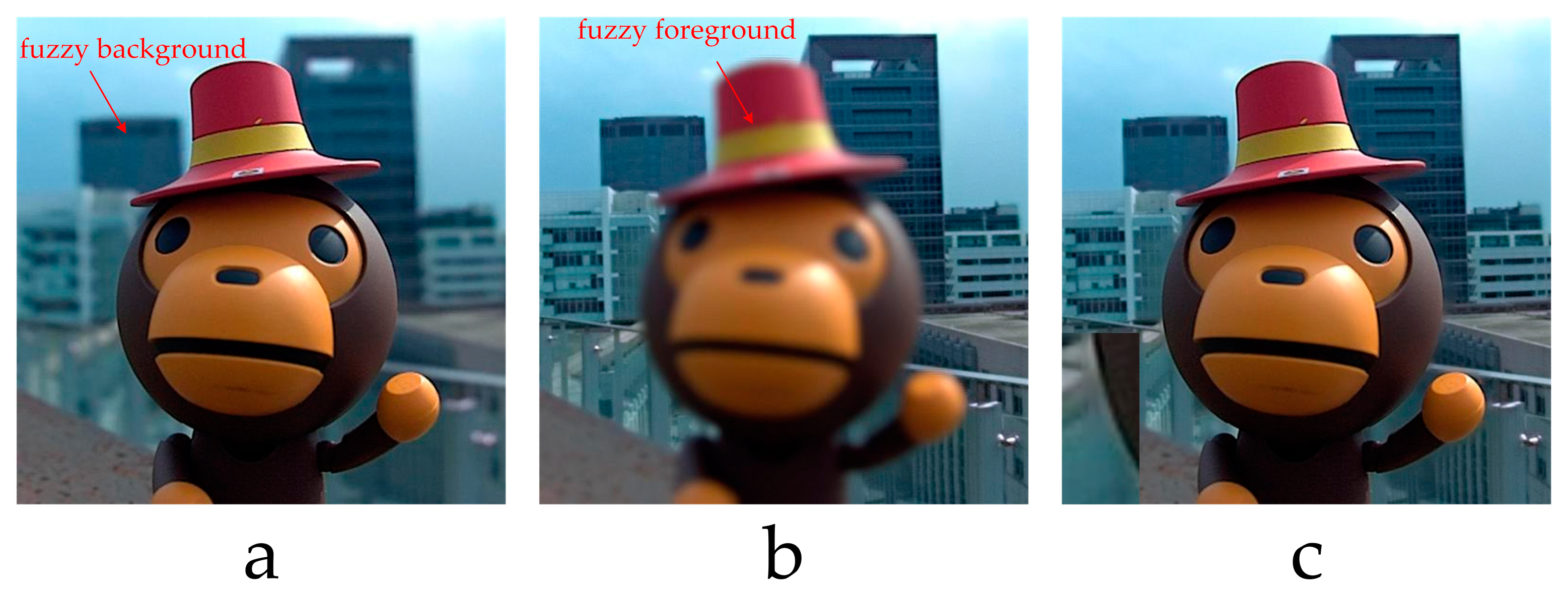
1. Introduction
2. The Related Work
- A region overlapping multi-source image fusion method based on BEMD block sharpness guidance is proposed for image fusion. First, the input image pairs are decomposed into intrinsic mode functions (BIMFs) and residuals, i.e., multiple two-dimensional image layers, respectively, using BEMD. Gaussian filtering is applied to the obtained image layer, the filtered image features are more obvious, and the noise caused in the interpolation process is also smoothed.
- A new fusion method is designed to improve the quality of the final fusion image, the filtered image is divided into different regions, and the improved Sobel weighted operator is used to calculate the image sharpness value of each region, which is an important reference for region selection.
- For the final region selection, we adopt the method of region stitching and region overlapping, which can reduce the influence of artifacts on the final fusion image. First, the area with a higher sharpness value is selected. Based on the articulation comparison strategy, gbimf and residual are fused by subregion splicing and region overlapping. The overlay layer is weighted to build the final fusion image.
3. Bidimensional Empirical Mode Decomposition
- Externally initialized, input image function f(x,y).
- If it is a multi-channel image such as a three-channel color image, the image is automatically layered and cyclically processed; if it is a single channel, it is directly input.
- Select the local maximum point and minimum point by sliding the local window.
- Process the local maximum and minimum points of the image separately through interpolation, obtaining the upper and lower envelope surfaces Emax(x,y) and Emin(x,y), and then calculating their mean value E(x,y).
- Input image f(x,y) minus the envelope mean E(x,y) to achieve a new intermediate variable L(x,y).
- Verify that L(x,y) meets BIMF’s filter termination criteria.
- L(x,y) = BIMFi is satisfied where (5) is performed to the residual image; otherwise, the following process is repeated until SD = 0.03 is satisfied:
- The decomposed BIMF components are summed and subtracted from the original plot to achieve the residual Rm(x,y) between the two.
- Input image F(x,y) can be represented by BEMD decomposition as
4. Multi-Source Image Fusion Algorithm
4.1. Selection Strategy by Sharpness Comparison
4.2. Improved Sobel Weighting Operator
4.3. The Maximum Sharpness Value Guidance of the Region Overlapping Fusion Algorithm
| Algorithm 1 Multi-source image fusion based on BEMD and region sharpness guidance region overlapping algorithm |
| Input: two source image I = (IA, IB) 1: a multi-channel image I 2: repeat 3: find all local maxima (minima) of each channel image of Ri−1 by comparing the values of each pixel and its neighbours in the 3 × 3 window centered on it 4: obtaining the upper and lower envelope surfaces Emax(x,y) and Emin(x,y) by Equations (1) and (2) 5: get a new intermediate variable L(x,y) by Equation (3) 6: obtain the i-th bimf and residue R 7: i = i + 1 8: until the residue Ri is a constant or a monotonic function, or thenumber of IMFs is more than a given threshold 9: Filter BIMFs and Residual through Equation (7) to get GBIMF and GRes 10: Use Sobel operator to calculate the clarity of GBIMF and GRES 11: Use Equation (19) to select a map with high definition 12: Fusion through overlapping segmentation Output: fused image If |
5. Experimental Results
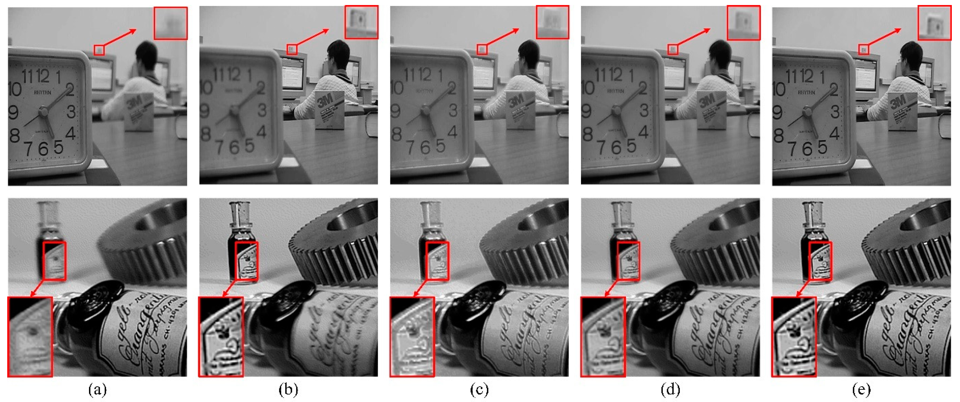
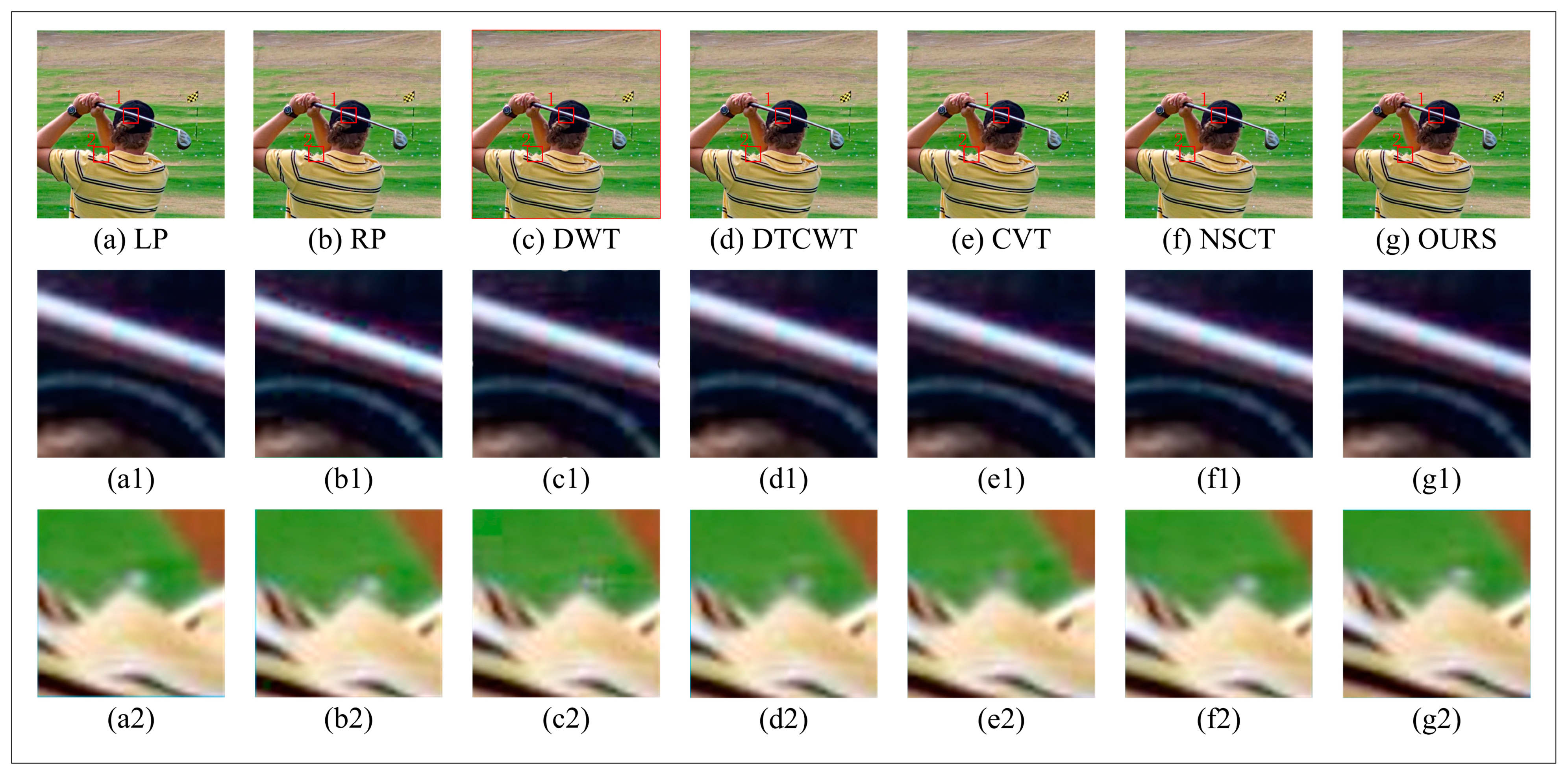
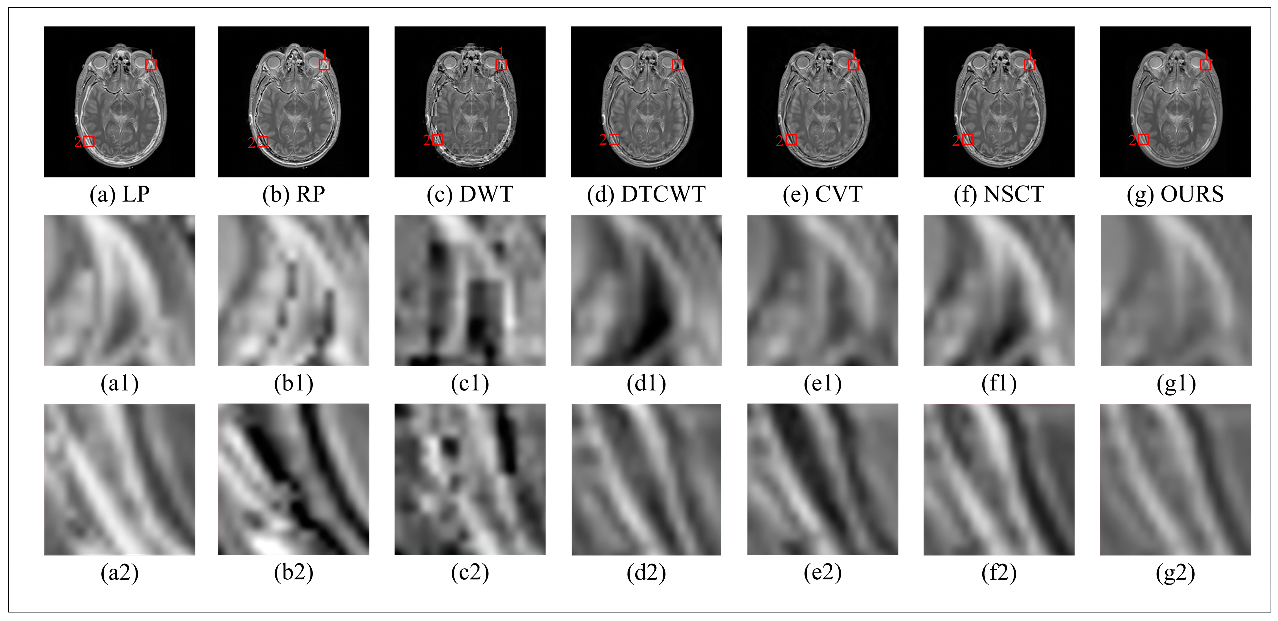
5.1. Qualitative Evaluation
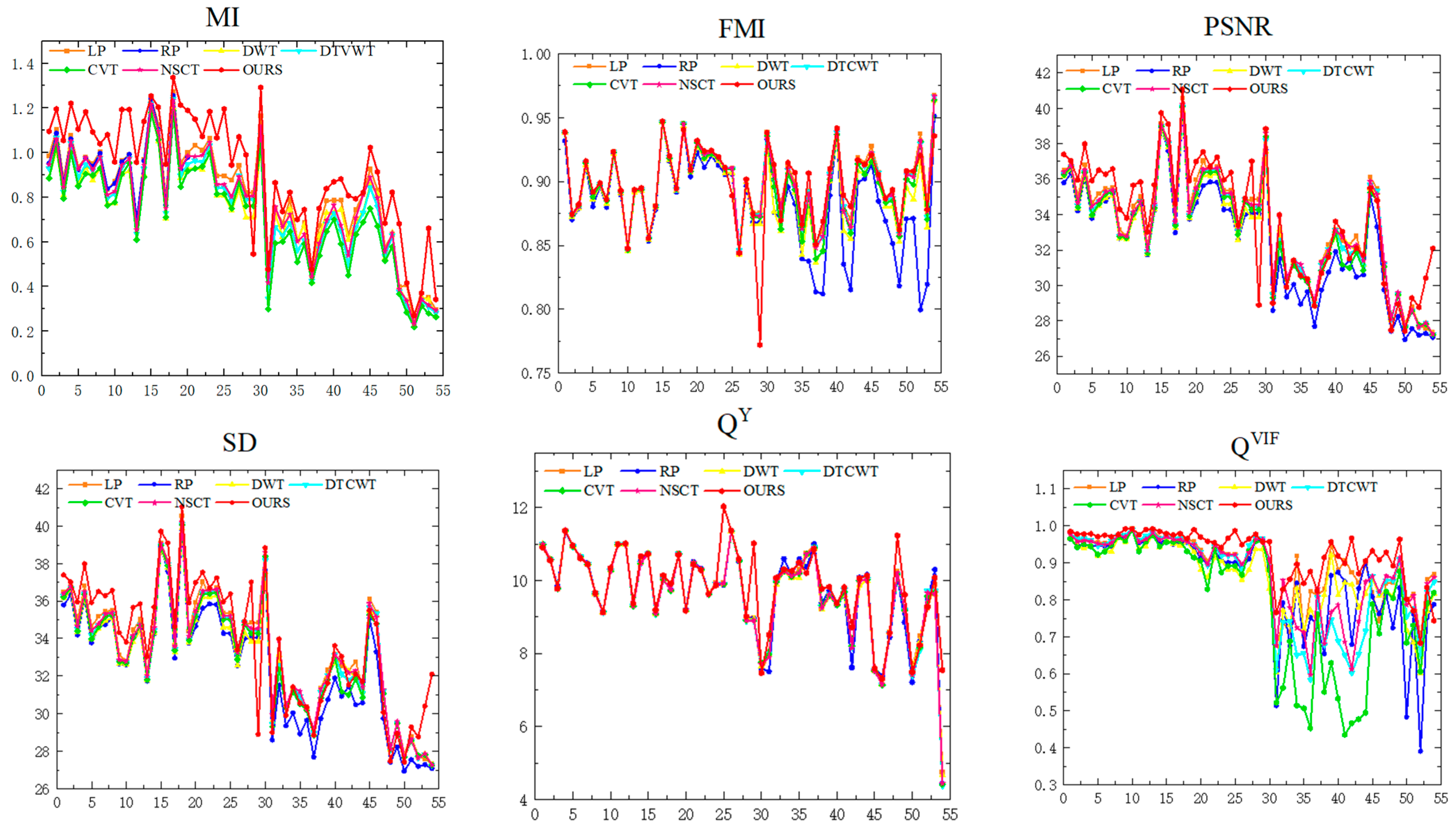
5.2. Quantitative Evaluation
6. Discussion and Conclusions
Author Contributions
Funding
Institutional Review Board Statement
Informed Consent Statement
Data Availability Statement
Conflicts of Interest
References
- Nunes, J.C.; Bouaoune, Y.; Delechelle, E.; Niang, O.; Bunel, P. Image analysis by bidimensional empirical mode decomposition. Image Vis. Comput. 2003, 21, 1019–1026. [Google Scholar] [CrossRef]
- Cheng, H.; Shen, H.; Meng, L.; Ben, C.; Jia, P. A Phase Correction Model for Fourier Transform Spectroscopy. Appl. Sci. 2024, 14, 1838. [Google Scholar] [CrossRef]
- Régal, X.; Cumunel, G.; Bornert, M.; Quiertant, M. Assessment of 2D Digital Image Correlation for Experimental Modal Analysis of Transient Response of Beams Using a Continuous Wavelet Transform Method. Appl. Sci. 2023, 13, 4792. [Google Scholar] [CrossRef]
- Xie, Q.; Hu, J.; Wang, X.; Zhang, D.; Qin, H. Novel and fast EMD-based image fusion via morphological filter. Vis. Comput. 2022, 39, 4249–4265. [Google Scholar] [CrossRef]
- Li, L.; Li, C.; Lu, X.; Wang, H.; Zhou, D. Multi-focus image fusion with convolutional neural network based on Dempster-Shafer theory. Optik 2023, 272, 170223. [Google Scholar] [CrossRef]
- Huang, W.; Jing, Z. Evaluation of focus measures in multi-focus image fusion. Pattern Recognit. Lett. 2007, 28, 493–500. [Google Scholar] [CrossRef]
- Ojdanić, D.; Zelinskyi, D.; Naverschnigg, C.; Sinn, A.; Schitter, G. High-speed telescope autofocus for UAV detection and tracking. Opt. Express 2024, 32, 7147–7157. [Google Scholar] [CrossRef]
- Pan, J.; Tang, Y.Y. A mean approximation based bidimensional empirical mode decomposition with application to image fusion. Digit. Signal Process. 2016, 50, 61–71. [Google Scholar]
- Garg, B.; Sharma, G. A quality-aware Energy-scalable Gaussian Smoothing Filter for image processing applications. Microsystems 2016, 45, 1–9. [Google Scholar] [CrossRef]
- Vairalkar, M.K.; Nimbhorkar, S.U. Edge detection of images using Sobel operator. Int. J. Emerg. Technol. Adv. Eng. 2012, 2, 291–293. [Google Scholar]
- Zhang, H.; Shen, H.; Yuan, Q.; Guan, X. Multispectral and SAR Image Fusion Based on Laplacian Pyramid and Sparse Representation. Remote Sens. 2022, 14, 870. [Google Scholar] [CrossRef]
- Pampanoni, V.; Fascetti, F.; Cenci, L.; Laneve, G.; Santella, C.; Boccia, V. Analysing the Relationship between Spatial Resolution, Sharpness and Signal-to-Noise Ratio of Very High Resolution Satellite Imagery Using an Automatic Edge Method. Remote. Sens. 2024, 16, 1041. [Google Scholar] [CrossRef]
- Liu, Y.; Liu, S.; Wang, Z. A general framework for image fusion based on multi-scale transform and sparse representation. Inf. Fusion 2015, 24, 147–164. [Google Scholar] [CrossRef]
- Ioannidou, S.; Karathanassi, V. Investigation of the Dual-Tree Complex and Shift-Invariant Discrete Wavelet Transforms on Quickbird Image Fusion. IEEE Geosci. Remote Sens. Lett. 2007, 4, 166–170. [Google Scholar] [CrossRef]
- Zhan, L.; Zhuang, Y.; Huang, L. Infrared and visible images fusion method based on discrete wavelet transform. J. Comput. 2017, 28, 57–71. [Google Scholar] [CrossRef]
- Zhao, X.; Jin, S.; Bian, G.; Cui, Y.; Wang, J.; Zhou, B. A Curvelet-Transform-Based Image Fusion Method Incorporating Side-Scan Sonar Image Features. J. Mar. Sci. Eng. 2023, 11, 1291. [Google Scholar] [CrossRef]
- Anandhi, D.; Valli, S. An algorithm for multi-sensor image fusion using maximum a posteriori and nonsubsampled contourlet transform. Comput. Electr. Eng. 2018, 65, 139–152. [Google Scholar] [CrossRef]
- Liu, Y.; Wang, L.; Cheng, J.; Li, C.; Chen, X. Multi-focus image fusion: A Survey of the state of the art. Inf. Fusion 2020, 64, 71–91. [Google Scholar] [CrossRef]
- Haghighat, M.B.A.; Aghagolzadeh, A.; Seyedarabi, H. A non-reference image fusion metric based on mutual information of image features. Comput. Electr. Eng. 2011, 37, 744–756. [Google Scholar] [CrossRef]
- Guo, W.; Xiong, N.; Chao, H.-C.; Hussain, S.; Chen, G. Design and Analysis of Self-Adapted Task Scheduling Strategies in Wireless Sensor Networks. Sensors 2011, 11, 6533–6554. [Google Scholar] [CrossRef]
- Wunsch, L.; Tenorio, C.G.; Anding, K.; Golomoz, A.; Notni, G. Data Fusion of RGB and Depth Data with Image Enhancement. J. Imaging 2024, 10, 73. [Google Scholar] [CrossRef] [PubMed]
- Liu, Y.; Chen, X.; Peng, H.; Wang, Z. Multi-focus image fusion with a deep convolutional neural network. Inf. Fusion 2017, 36, 191–207. [Google Scholar] [CrossRef]
- Bhutto, J.A.; Lianfang, T.; Du, Q.; Soomro, T.A.; Lubin, Y.; Tahir, M.F. An enhanced image fusion algorithm by combined histogram equalization and fast gray level grouping using multi-scale decomposition and gray-PCA. IEEE Access 2020, 8, 157005–157021. [Google Scholar] [CrossRef]
- Bhutto, J.A.; Tian, L.; Du, Q.; Sun, Z.; Yu, L.; Soomro, T.A. An improved infrared and visible image fusion using an adaptive contrast enhancement method and deep learning network with transfer learning. Remote Sens. 2022, 14, 939. [Google Scholar] [CrossRef]
- Bhutto, J.A.; Tian, L.; Du, Q.; Sun, Z.; Yu, L.; Tahir, M.F. CT and MRI medical image fusion using noise-removal and contrast enhancement scheme with convolutional neural network. Entropy 2022, 24, 393. [Google Scholar] [CrossRef]


| Region | Stack Layer |
|---|---|
| a,h,p,v | 1 |
| b,f,I,o,q,u | 2 |
| c,d,e,r,s,t | 3 |
| j,n | 4 |
| k,l,m | 6 |
| Methods | MI | FMI | PSNR | SD | QY | QVIF | TIME |
|---|---|---|---|---|---|---|---|
| LP | 0.9811 | 0.9009 | 35.5011 | 10.2568 | 0.9657 | 1.5879 | 0.0170 |
| RP | 0.9678 | 0.8972 | 34.9039 | 10.2615 | 0.9547 | 1.5732 | 0.3491 |
| DWT | 0.9075 | 0.8989 | 34.9948 | 10.2527 | 0.9461 | 1.5197 | 0.7552 |
| DTCWT | 0.9401 | 0.9006 | 35.1847 | 10.2470 | 0.9647 | 1.5482 | 1.4975 |
| CVT | 0.9041 | 0.9001 | 35.1226 | 10.2472 | 0.9447 | 1.5347 | 6.2568 |
| NSCT | 0.9526 | 0.9006 | 35.2878 | 10.2500 | 0.9616 | 1.5667 | 17.1029 |
| Ours | 1.1235 | 0.9010 | 36.4724 | 10.2797 | 0.9791 | 1.6023 | 1.0652 |
| Methods | MI | FMI | PSNR | SD | QY | QVIF | TIME |
|---|---|---|---|---|---|---|---|
| LP | 0.9519 | 0.9024 | 35.7084 | 9.7644 | 0.9264 | 1.5326 | 0.0315 |
| RP | 0.9405 | 0.8964 | 34.8109 | 9.7586 | 0.9148 | 1.5020 | 0.0916 |
| DWT | 0.8481 | 0.8970 | 34.9988 | 9.7636 | 0.8883 | 1.4222 | 0.1350 |
| DTCWT | 0.8969 | 0.9015 | 35.4490 | 9.7546 | 0.9260 | 1.4885 | 0.3092 |
| CVT | 0.9476 | 0.9004 | 35.3754 | 9.7594 | 0.9025 | 1.4694 | 1.7779 |
| NSCT | 0.9138 | 0.9009 | 35.5876 | 9.7618 | 0.9275 | 1.5062 | 4.8504 |
| Ours | 1.0506 | 0.8897 | 35.7860 | 10.1688 | 0.9616 | 1.5071 | 0.3329 |
| Methods | MI | FMI | PSNR | SD | QY | QVIF | TIME |
|---|---|---|---|---|---|---|---|
| LP | 0.7116 | 0.8965 | 31.9464 | 9.4535 | 0.8205 | 0.9016 | 0.0570 |
| RP | 0.7171 | 0.8689 | 30.6170 | 9.4336 | 0.7635 | 0.8500 | 0.0259 |
| DWT | 0.6736 | 0.8828 | 31.8465 | 9.3930 | 0.7918 | 0.7842 | 0.0755 |
| DTCWT | 0.6272 | 0.8928 | 31.7666 | 9.4326 | 0.6999 | 0.7896 | 0.1352 |
| CVT | 0.5818 | 0.8873 | 31.4522 | 9.4282 | 0.5682 | 0.7174 | 0.7658 |
| NSCT | 0.6685 | 0.8929 | 32.0096 | 9.4237 | 0.7483 | 0.8430 | 1.6713 |
| Ours | 0.7819 | 0.8984 | 32.1865 | 9.5780 | 0.9616 | 0.9579 | 1.1853 |
| Methods | MI | FMI | PSNR | SD | QY | QVIF | TIME |
|---|---|---|---|---|---|---|---|
| LP | 0.4047 | 0.8052 | 28.4983 | 8.4960 | 0.8295 | 0.9444 | 0.0061 |
| RP | 0.3667 | 0.8562 | 27.6723 | 8.3892 | 0.6932 | 0.8668 | 0.0370 |
| DWT | 0.3844 | 0.8923 | 28.4818 | 8.4584 | 0.7630 | 0.7499 | 0.0633 |
| DTCWT | 0.3756 | 0.9013 | 28.4693 | 8.3869 | 0.8079 | 0.7787 | 0.1444 |
| CVT | 0.3513 | 0.8988 | 28.4634 | 8.3969 | 0.7668 | 0.7252 | 0.8411 |
| NSCT | 0.3864 | 0.9025 | 28.4964 | 8.4097 | 0.8275 | 0.8329 | 2.3144 |
| Ours | 0.5300 | 0.8991 | 29.3041 | 8.9991 | 0.8328 | 0.9826 | 1.0568 |
| Data Set | Methods | MI | FMI | PSNR | SD | QY | QVIF | TIME |
|---|---|---|---|---|---|---|---|---|
| Color multi-focus set | CNN | 1.1512 | 0.8913 | 36.4127 | 10.1764 | 0.9801 | 1.6011 | 85.1135 |
| Ours | 1.1235 | 0.9010 | 36.4724 | 10.2797 | 0.9791 | 1.6023 | 1.0652 | |
| Gray multi-focus set | CNN | 0.9976 | 0.8762 | 35.4385 | 9.9277 | 0.9386 | 1.4995 | 49.1315 |
| Ours | 1.0506 | 0.8897 | 35.7860 | 10.1688 | 0.9616 | 1.5071 | 0.3329 | |
| Medical multi-modal set | CNN | 0.7362 | 0.8928 | 31.4792 | 9.5564 | 0.7982 | 0.8869 | 24.9169 |
| Ours | 0.7819 | 0.8984 | 32.1865 | 9.5780 | 0.9616 | 0.9579 | 1.1853 | |
| Infrared and visual sets | CNN | 0.6283 | 0.7936 | 28.5707 | 8.5180 | 0.7920 | 0.8163 | 23.1417 |
| Ours | 0.5300 | 0.8991 | 29.3041 | 8.9991 | 0.8328 | 0.9826 | 1.0568 |
Disclaimer/Publisher’s Note: The statements, opinions and data contained in all publications are solely those of the individual author(s) and contributor(s) and not of MDPI and/or the editor(s). MDPI and/or the editor(s) disclaim responsibility for any injury to people or property resulting from any ideas, methods, instructions or products referred to in the content. |
© 2024 by the authors. Licensee MDPI, Basel, Switzerland. This article is an open access article distributed under the terms and conditions of the Creative Commons Attribution (CC BY) license (https://creativecommons.org/licenses/by/4.0/).
Share and Cite
Guo, X.-T.; Duan, X.-J.; Kong, H.-H. Multi-Source Image Fusion Based on BEMD and Region Sharpness Guidance Region Overlapping Algorithm. Appl. Sci. 2024, 14, 7764. https://doi.org/10.3390/app14177764
Guo X-T, Duan X-J, Kong H-H. Multi-Source Image Fusion Based on BEMD and Region Sharpness Guidance Region Overlapping Algorithm. Applied Sciences. 2024; 14(17):7764. https://doi.org/10.3390/app14177764
Chicago/Turabian StyleGuo, Xiao-Ting, Xu-Jie Duan, and Hui-Hua Kong. 2024. "Multi-Source Image Fusion Based on BEMD and Region Sharpness Guidance Region Overlapping Algorithm" Applied Sciences 14, no. 17: 7764. https://doi.org/10.3390/app14177764
APA StyleGuo, X.-T., Duan, X.-J., & Kong, H.-H. (2024). Multi-Source Image Fusion Based on BEMD and Region Sharpness Guidance Region Overlapping Algorithm. Applied Sciences, 14(17), 7764. https://doi.org/10.3390/app14177764