Analysis of Longitudinal Braking Stability of Lightweight Liquid Storage Mini-Track Vehicles

Abstract

In this study, a theoretical model was established for longitudinal braking stability (LBS) of a lightweight liquid storage mini-track vehicle to investigate its behaviors. The influence of the tank liquid filling ratio (TLR), initial velocity (IV), and initial braking deceleration (IBD) on the LBS of the tracked vehicle was studied via FLUENT simulation. The simulation results showed that when the IV and the IBD were constant, the TLR significantly affected the braking efficiency. Conversely, when the TLR was 0.7, the braking efficiency decreased by 32%, resulting in the worst LBS. The braking efficiency at different IVs decreased by ~30% when using a constant IBD and TLR, and the braking stability exhibited little difference. Further, the braking efficiency decreased noticeably with increasing IBD; meanwhile, the braking longitudinal stability worsened. When the IBD was increased to 5 m⋅s⁻², the braking efficiency decreased by 48.4%. The road experiment showed that when the tracked vehicle was accelerated and braked under limit conditions, the stability requirements were met. Finally, by combining the simulation and road experiment, the driving parameters of the tracked vehicle that could satisfy the LBS were obtained.

1. Introduction

A lightweight liquid storage mini-track vehicle that can carry a power source and rescue tools is the research object in this study. Such a vehicle can be used to enable rescue troops to cross obstacles, and rapidly reach the complex and narrow disaster site. Owing to the need to reserve a large amount of hydraulic oil in the tank during the rescue operations, studies on the driving stability of tracked vehicles are quite different from those concerned with ordinary tracked vehicles. This is especially true when it comes to the braking of tracked vehicles, because the influence of the liquid inertial force makes the liquid center of gravity move forward, which affects the tracked vehicle. Therefore, in this scenario, the tracked vehicle is subjected to both its inertia and the liquid impact force, which affect its braking stability.

Many studies on the influence of liquid force on the driving stability of liquid storage vehicles have been carried out to date. For instance, Wan et al. [1] initially established a complex two-way coupled dynamic model for tank trucks and discussed various liquid motion characteristics and their effects on the longitudinal braking performance. Shi et al. [2] concluded that when a rail vehicle passed a curve at a speed higher than the equilibrium speed, the liquid slosh led to the increase in the unbalance effect. Tractive analysis showed that liquid sloshing significantly influenced the load distribution between the front and rear trucks. For example, Wu Wen et al. [3] designed an experimental rig for measuring the dynamic rocking force and slosh torque of liquid in the tank. The rig was able to achieve accurate real-time measurements of the three-dimensional (3D) dynamic signals of the shaking force and shaking movement of liquid in the tank. Further, the author studied the dynamic characteristics of liquid shaking under different working conditions by carrying out many experiments. Consequently, a reliable measurement method and experimental basis were provided for conducting an entire-system dynamic analysis and studying the control of vehicles. Li [4] established a liquid dynamic model by using FLUENT and used it to study the longitudinal stability of the liquid storage vehicle under braking conditions. The main factors affecting the braking stability were studied by changing single variables, such as the speed and acceleration, of the liquid storage vehicle. Next, Azadi et al. [5] also established a tank fluid slosh model using FLUENT and coupled the liquid with a liquid storage vehicle for numerical simulation. The model was used to observe the directional response and roll stability of a semi-trailer under different parameters and conditions.

The effect of the filling ratio of the liquid tank on vehicle stability has also been studied extensively. For example, Zhou and Wang et al. [6,7] established a multi-degree-of-freedom dynamic model of vehicle–liquid coupling. The tank liquid filling ratio (TLR) and lateral acceleration were found to have a significant influence on the vehicle roll dynamics and stability. Zheng et al. [8] studied how the instantaneous liquid impact affected the vehicle roll stability. It was found that the declining degree of roll stability of all tank vehicles increased with the TLR. Li [9] used the smooth particle fluid dynamics method to simulate the sloshing of the liquid in the tank under excitation. HyperMesh 2023 was used to establish a liquid tank calculation model under braking conditions. The study showed that the liquid sloshing in the tank was the most intense when the filling ratio was 75%. Chen [10] established a numerical calculation model of liquid slosh based on the finite volume method for the studied vehicle liquid tank; FLUENT was used to simulate and study the slosh characteristics of the liquid. Characteristics were studied under various braking accelerations, lateral accelerations, and filling ratios. The results showed that the impact of the flow field on the structure increased with the increase in braking excitation and lateral excitation. Moreover, the impact on the structure was the largest when the TLR ranged between 0.7 and 0.9. Further, Feng [11] established a liquid slosh model in a tank based on an equivalent mass-spring-damping system. The model was combined with a liquid slosh prediction model utilizing an artificial neural network, which resulted in a longitudinal dynamic model of the liquid tank vehicle containing a wave plate tank. FLUENT was used to simulate and study the effects of TLR and ground adhesion coefficient on the vehicle braking performance. Finally, Zhang et al. [12] also used FLUENT to establish a stability model of the liquid storage vehicle during braking and turning actions. It was concluded that the liquid exhibited the greatest influence on the stability of the liquid storage vehicle when the TLR of the tank ranged between 30% and 75%.

Based on the investigation of the relevant literature, it was determined that the TLR significantly impacts the longitudinal braking stability (LBS) of a liquid storage vehicle. However, the systematic research on the LBS of a liquid storage tracked vehicle have rarely been carried out to date. Therefore, based on previous research results, in this study, the LBS of a lightweight liquid storage mini-track vehicle was systematically explored. The term LBS of a tracked vehicle refers to the braking deceleration stability of the tracked vehicle [13]. The main factors affecting the longitudinal stability of a tracked vehicle are road conditions, TLR, initial velocity (IV), and initial braking deceleration (IBD). In this study, a lightweight liquid storage mini-track vehicle was designed and used as the research object. First, a theoretical model of the LBS of the tracked vehicle under liquid impact was established. Next, the influences of TLR, IV, and IBD on the LBS of the hydraulic tracked vehicle were studied. Finally, it was intended that this study should provide the theoretical guidance and data support required for in-depth studies on the dynamic stability of lightweight liquid storage mini-track vehicles.

The outline of this paper is as follows. Section 2 presents the LBS model. Section 3 outlines the simulation results. Section 4 discusses the road experiment and Section 5 provides the conclusions.

2. Analysis of LBS

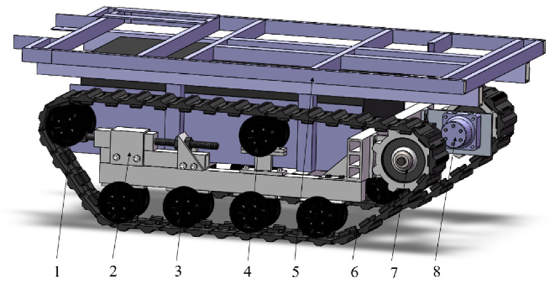
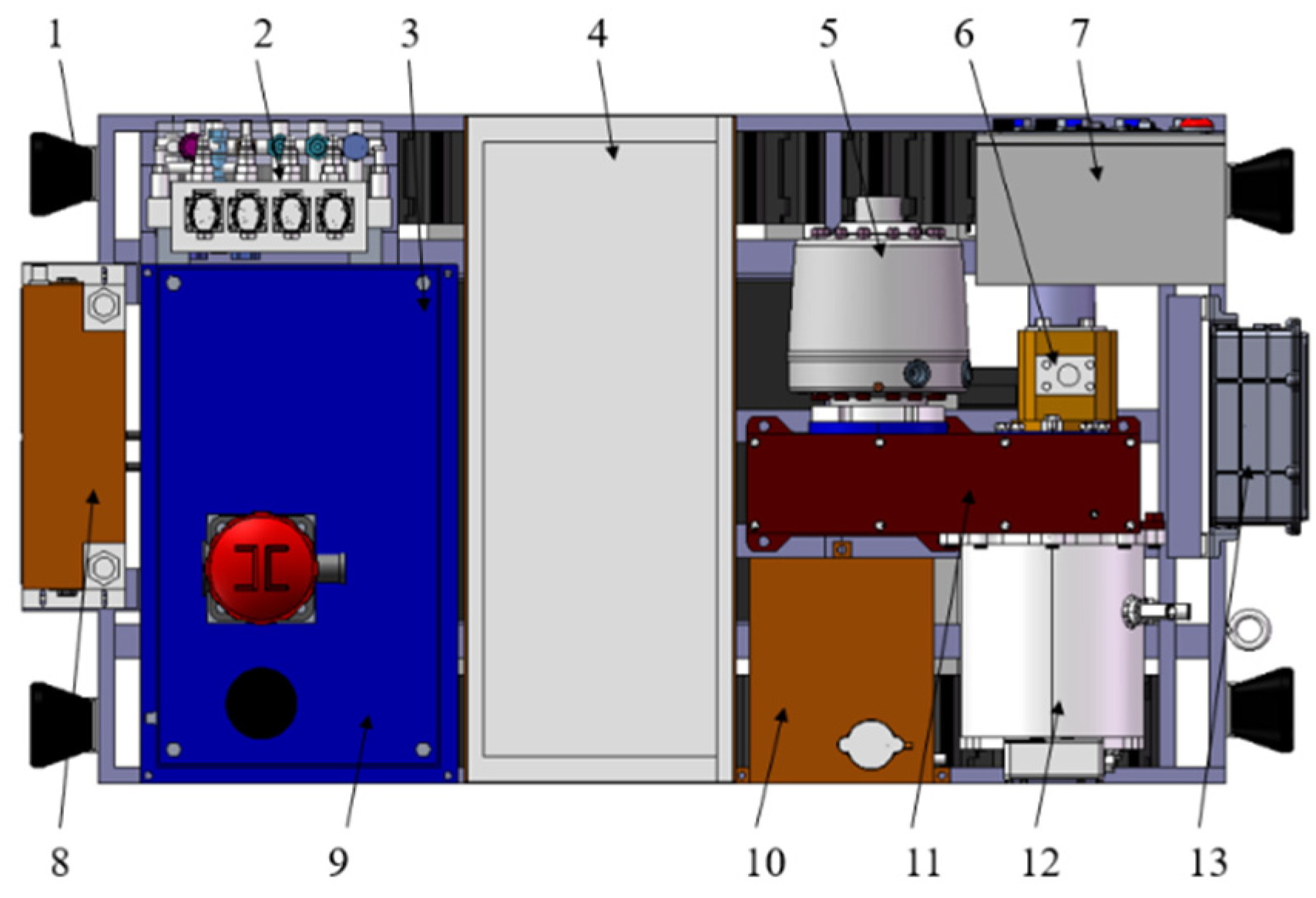
2.1. Tracked Vehicle Structure and Onboard Layout

The chassis of the tracked vehicle is primarily composed of guide wheels, load support wheels, drive wheels, belt support wheels, track, frame, a tensioning buffer device, and drive motor (see Figure 1). The main parameters are as follows: the overall dimensions were 1500 mm × 800 mm × 1000 mm, liquid tank size was 800 mm × 340 mm × 340 mm, and the maximum speed was above 5 km⋅h⁻¹.

Figure 2 shows the layout of each component on the chassis. The chassis frame is the core supporting part of the tracked vehicle. The working parts, such as the liquid tank, reducer, high/low-pressure pump, and motor, were mounted on the chassis frame. The remaining components, except for the liquid tank, were regarded as a fixed load. The liquid in the tank shows a dynamic impact on the vehicle due to the change in the speed of the tracked vehicle. Therefore, it was necessary to study the influence of liquid impact force on the dynamic stability of the tracked vehicle.

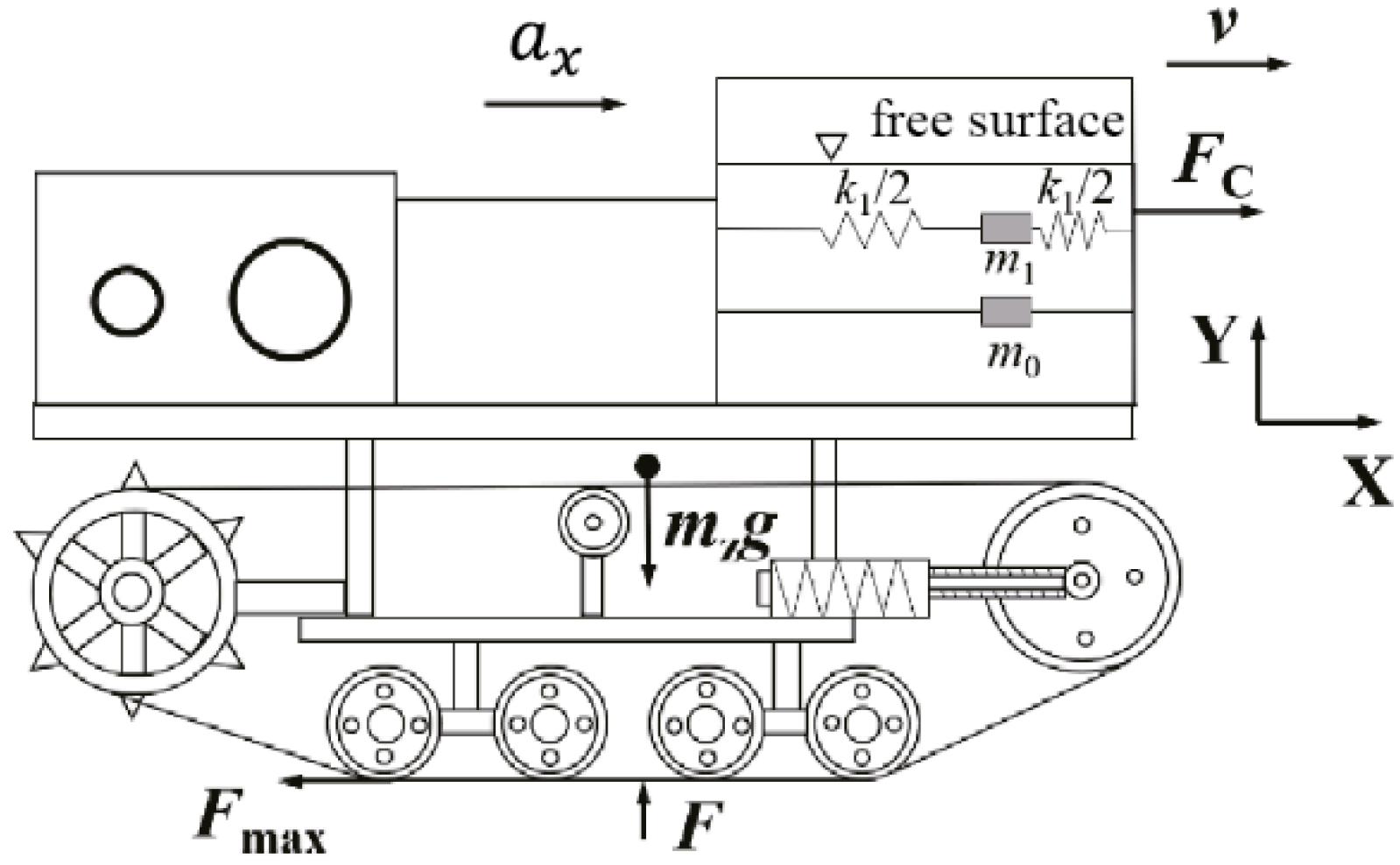
2.2. Mathematical Modeling

The braking force diagram of the tracked vehicle is shown in Figure 3.

The effective braking force F_x satisfies Newton’s second law, as follows:

$$F_x=m_z{a}_x$$

(1)

where m_z is the total mass of the tracked vehicle when the fluid is loaded in the tank and a_x denotes the effective braking deceleration.

Owing to the influence of liquid slosh on the longitudinal force, the effective braking force was obtained as follows:

$$F_x=F_{max}-F_c$$

(2)

where F_c is the longitudinal impact force of liquid oscillation on the tracked vehicle tank wall and F_max denotes the maximum braking force exerted on the ground, calculated as follows:

$$F_{max}=m_{z}g\phi$$

(3)

where φ is the ground adhesion coefficient and φ = 0.5 is used in this study.

By combining Equations (1)–(3), the expression for effective braking deceleration a_x of the tracked vehicle was obtained:

$$a_x=g\phi -{\displaystyle \frac{F_c}{m_z}}$$

(4)

According to Equation (4), under the impact of liquid, effective braking deceleration is negatively correlated with longitudinal impact force F_c. The larger the F_c, the smaller the effective braking deceleration. Its increase also led to the decrease in the LBS and increase in the braking time.

Since the liquid impact in the tank affects the LBS of the tracked vehicle, it is necessary to study the kinematic and dynamic characteristics of the liquid in the tank when the tracked vehicle is driving on any road surface. The equivalent spring-mass mechanical model should be used to simulate the oscillations of the liquid in the tank [14]. Such liquid motion includes the oscillation term and the longitudinal impact force term, and can be expressed as follows:

$$m_1{\displaystyle \frac{d^{2}x}{d{t}^2}}+c_1{\displaystyle \frac{dx}{dt}}+k_{1}x+F_c=-m_1{a}_x$$

(5)

where m₁ is the liquid mass; t is the time; c₁ is the spring damping coefficient; and k₁ is the spring stiffness coefficient.

The longitudinal impact force F_c of the liquid in the tank can be calculated as follows:

$$F_c=\eta m_1{x}_0{\left({\displaystyle \frac{x}{x_0}}\right)}^{2n-1}$$

(6)

where η is a normal parameter coefficient; m₁ is the spring mass; x₀ = w/2; w is the tank width (the distance between the front and back walls); x denotes the change in the spring length; and n is a positive integer significantly greater than 1 (n >> 1).

Equation (6) indicates that the longitudinal impact force F_c is related to the liquid mass, the longitudinal distance of the tank, the oscillation displacement of the liquid, and the inertial force of the liquid. Therefore, the longitudinal impact force F_c is needed to evaluate the longitudinal stability of a tracked vehicle during braking, and the theoretical calculation method of F_c is given in the subsequent text.

2.3. Theoretical Solution of the Longitudinal Impact Force of Tank Liquid According to a Literature Study [4]

During the track vehicle braking, the tank liquid produces a turbulent impact. The governing equations of fluids required for studying turbulence problems are continuity, momentum, and turbulence equations [2]. They are given as follows:

• Continuity equation:

$${\displaystyle \frac{\partial u_i}{\partial x_i}}+{\displaystyle \frac{\partial u_j}{\partial x_j}}+{\displaystyle \frac{\partial u_k}{\partial x_k}}=0$$

(7)

where $u_i, u_j,\mathrm{and}{u}_{k }$ are velocity vectors in the x, y, and z directions, respectively, and are coordinate values in the x, y, and z directions.

• Momentum conservation equation:

$$\begin{array}{c}{\displaystyle \frac{\partial u_i}{\partial t}}+u_i{\displaystyle \frac{\partial u_i}{\partial x_i}}+u_j{\displaystyle \frac{\partial u_i}{\partial x_j}}+u_k{\displaystyle \frac{\partial u_i}{\partial x_k}}=F_i-{\displaystyle \frac{1}{\rho }}{\displaystyle \frac{\partial p}{\partial x}}+{\displaystyle \frac{\mu }{\rho }}\left[{\displaystyle \frac{{\partial }^2{u}_i}{\partial {x_i}^2}}+{\displaystyle \frac{{\partial }^2{u}_i}{\partial {x_j}^2}}+{\displaystyle \frac{{\partial }^2{u}_i}{\partial {x_k}^2}}\right]\\ {\displaystyle \frac{\partial u_j}{\partial t}}+u_i{\displaystyle \frac{\partial u_j}{\partial x_i}}+u_j{\displaystyle \frac{\partial u_j}{\partial x_j}}+u_k{\displaystyle \frac{\partial u_j}{\partial x_k}}=F_j-{\displaystyle \frac{1}{\rho }}{\displaystyle \frac{\partial p}{\partial x}}+{\displaystyle \frac{\mu }{\rho }}\left[{\displaystyle \frac{{\partial }^2{u}_j}{\partial {x_i}^2}}+{\displaystyle \frac{{\partial }^2{u}_j}{\partial {x_j}^2}}+{\displaystyle \frac{{\partial }^2{u}_j}{\partial {x_k}^2}}\right]\\ {\displaystyle \frac{\partial u_k}{\partial t}}+u_i{\displaystyle \frac{\partial u_k}{\partial x_i}}+u_j{\displaystyle \frac{\partial u_k}{\partial x_j}}+u_k{\displaystyle \frac{\partial u_k}{\partial x_k}}=F_k-{\displaystyle \frac{1}{\rho }}{\displaystyle \frac{\partial p}{\partial x}}+{\displaystyle \frac{\mu }{\rho }}\left[{\displaystyle \frac{{\partial }^2{u}_k}{\partial {x_i}^2}}+{\displaystyle \frac{{\partial }^2{u}_k}{\partial {x_j}^2}}+{\displaystyle \frac{{\partial }^2{u}_k}{\partial {x_k}^2}}\right]\end{array}$$

(8)

where F_i, F_j, and F_k are components of force in the x, y, and z directions, respectively; ρ is the density; μ is the dynamic viscosity; and p is the liquid pressure.

• Parametric equation of turbulence model

K (turbulent kinetic energy) equation:

$$\rho {\displaystyle \frac{\partial K}{\partial t}}+\rho u_j{\displaystyle \frac{\partial K}{x_j}}={\displaystyle \frac{\partial }{\partial x_i}}\left[\left[\mu +{\displaystyle \frac{{\mu }_t}{{\sigma }_K}}\right]{\displaystyle \frac{\partial K}{\partial x_j}}\right]+{\mu }_t{\displaystyle \frac{\partial u_i}{\partial x_j}}\left[{\displaystyle \frac{\partial u_i}{\partial x_j}}+{\displaystyle \frac{\partial u_j}{\partial x_i}}\right]-\rho \epsilon$$

(9)

ε (dissipation rate) equation:

$$\rho {\displaystyle \frac{\partial \epsilon }{\partial t}}+\rho u_k{\displaystyle \frac{\partial \epsilon }{x_k}}={\displaystyle \frac{\partial }{\partial x_k}}\left[\left[\mu +{\displaystyle \frac{{\mu }_t}{{\sigma }_{\epsilon }}}\right]{\displaystyle \frac{\partial \epsilon }{\partial x_k}}\right]+{\displaystyle \frac{c_1\epsilon }{K}}{\mu }_t{\displaystyle \frac{\partial u_i}{\partial x_j}}\left[{\displaystyle \frac{\partial u_i}{\partial x_j}}+{\displaystyle \frac{\partial u_j}{\partial x_i}}\right]-c_2\rho {\displaystyle \frac{{\epsilon }^2}{K}}$$

(10)

where K is the Reynolds mean velocity component; μ_t is the turbulence viscosity coefficient; $-\rho \epsilon$ is the dissipation term; and ${\sigma }_K,{\sigma }_{\epsilon }, c_1, \mathrm{and} c_2$ are the empirical constants of the standard K–ε turbulence model.

The longitudinal impact force F_c of the liquid can be obtained through the fluid control equation; however, it is difficult to solve the nonlinear and partial differential problems. Therefore, since the fluid simulation software FLUENT 2023 R1 integrates all the equations outlined above, it can simulate the fluid flow, and thus accurate CFD analysis results can be obtained. Therefore, solving the longitudinal impact force of the liquid in the tank via FLUENT 2023 R1 can improve the solving efficiency.

3. Simulation of LBS

3.1. Simulation Parameters

Liquid slosh is a type of movement generated by the fluid with the free liquid surface in a specific space [15]. The longitudinal impact force of the liquid of the lightweight liquid storage mini-track vehicles was simulated and solved. Both the transverse and horizontal sections of the liquid tank were rectangular. Therefore, to simplify the modeling and reduce the computational cost of the simulation process, the 3D model of the liquid tank was converted into a 2D model pair through the mass method.

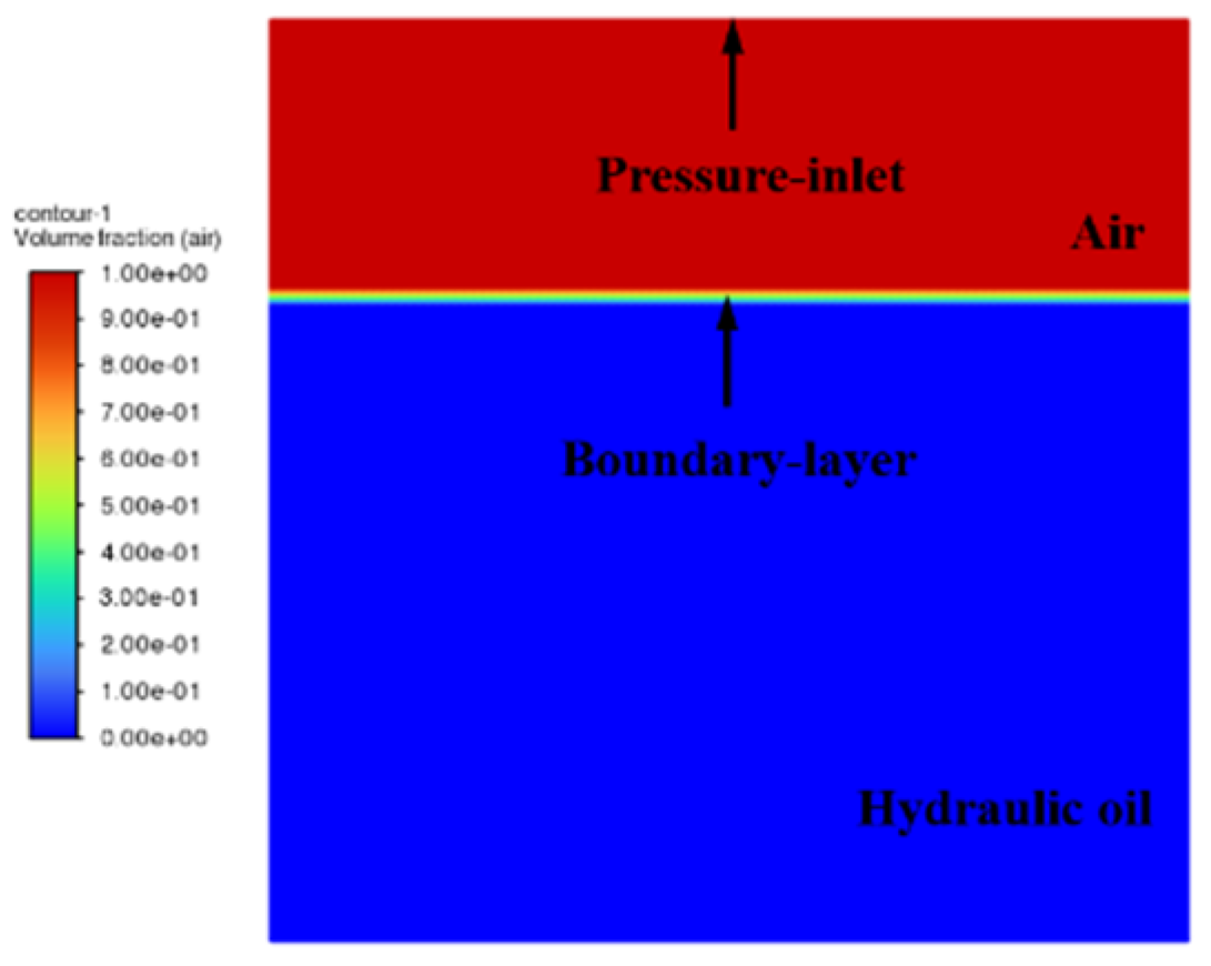
3.1.1. Liquid Tank Model and Boundary Conditions

The CAE pre-processing software ICEM CFD 2023 R1was used to establish the liquid tank model. The longitudinal section of the tank was 0.34 m long and 0.34 m high. The liquid tank model and boundary conditions were set as shown in Figure 4. The free liquid surface of the liquid tank at the initial moment was the boundary line of the two-phase flow. Furthermore, the boundary of the 2D liquid slop model included the pressure inlet boundary condition, ensuring the constant pressure in the tank and the wall condition, restricting the liquid slop deformation.

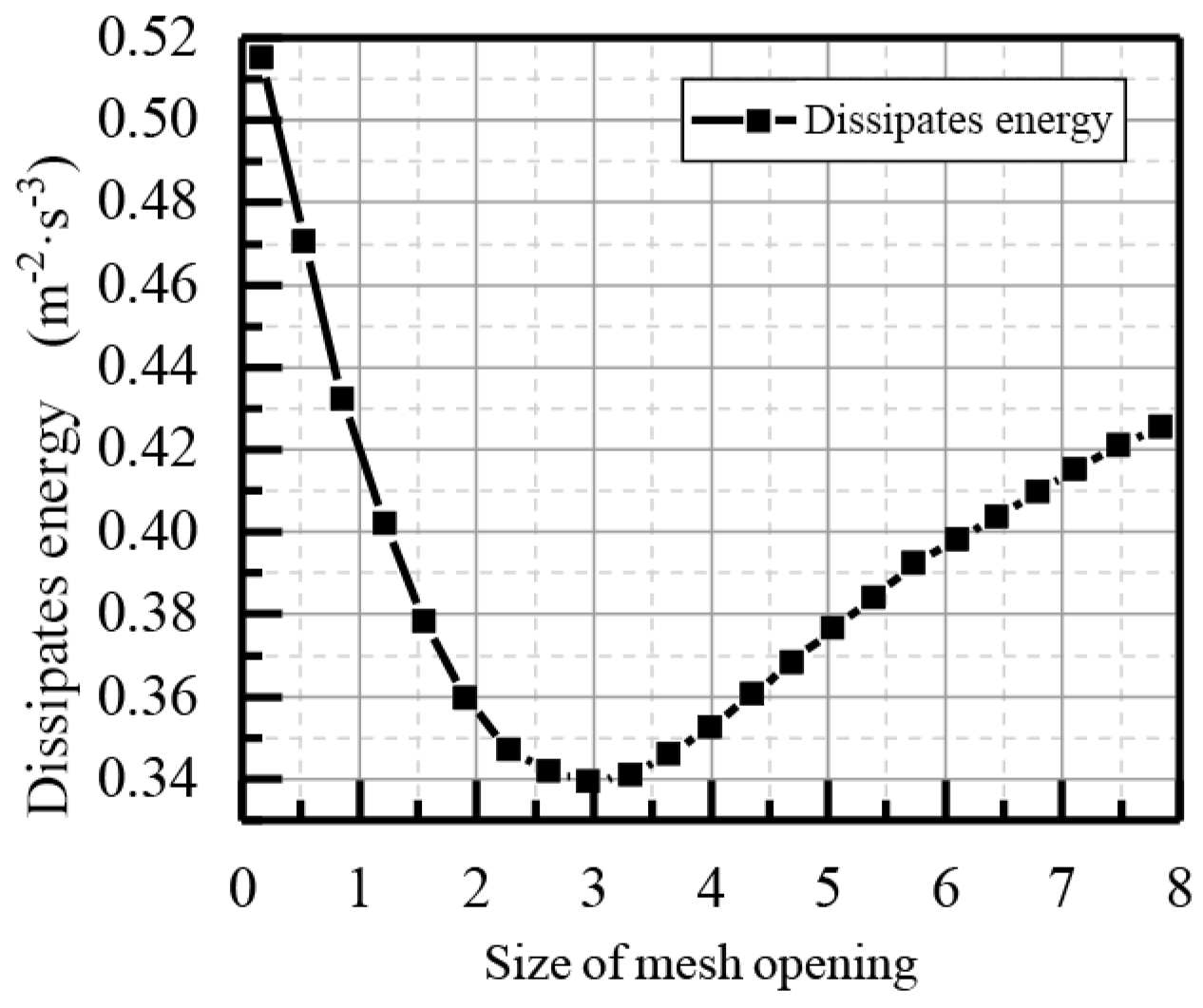
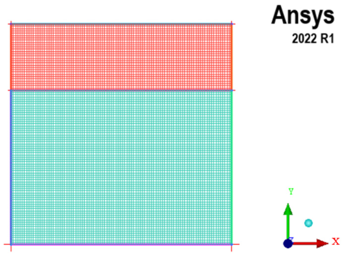
3.1.2. Mesh Precision Design and Mesh Division

Notably, liquid oscillation is a turbulence problem; therefore, turbulent dissipation energy was used as an evaluation index for grid accuracy design [14]. Lower turbulent dissipation energy corresponded to a higher mesh accuracy. By using the turbulent dissipation energy function and ANSYS mesh size design, the mesh was designed accurately. The corresponding relationship between turbulent dissipated energy and mesh size is given in Figure 5.

Figure 5 shows that when the mesh size was between 2.2 and 3.2 mm, the turbulent dissipation energy was rather stable and relatively low, while the mesh accuracy was high. The cell mesh size of 3 mm was selected to grid the liquid and air in the tank (Figure 6). The mesh consisted of 12,656 elements, implying a high mesh quality.

3.1.3. Setting of the Key Parameters

After the completion of the grid division, it was imported into FLUENT 2023 for simulation calculation. Before the simulation, simulation parameters were required to be set. In this study, a pressure-based solver was used and an implicit solution was adopted. The SIMPLE algorithm was used to solve the flow field, and liquid slosh was considered as a transient problem. Transient and gravity were activated, and the gravity acceleration in the Y direction was set to −9.81 m⋅s⁻². The standard k–ε turbulence model was selected.

It is noteworthy that the main objective of this study was to solve the multiphase flow model problem; therefore, relevant parameters of the multiphase flow model were required to be set. The volume of fluid (VOF) model was used, with the number of phases set to two; the first phase was set as air while the second was hydraulic oil. The specific density of air was 1.225 kg⋅m⁻³, with its viscosity being 1.7894 × 10⁻⁵ kg⋅(m⋅s)⁻¹. The density and viscosity of hydraulic oil were 876 kg⋅m⁻³ and 0.048 kg⋅(m⋅s)⁻¹, respectively.

3.1.4. Simulation Experimental Data

Equations (4)–(6) show that effective braking deceleration is related to hydraulic oil quality, IV of the tracked vehicle, and braking deceleration. Therefore, the influence of the TLR, IV of the tracked vehicles, and braking deceleration on the longitudinal stability of the studied vehicle during braking was investigated through the control variable method. The TLR of the tracked vehicle was set between 0.5 and 0.9, the IV was 1 km⋅h⁻¹, and the IBD was 3 to 5 m⋅s⁻². The experimental groups were formed as presented in

Table 1. Parameter settings of different experimental groups.

Experiment Group 1			Experiment Group 2			Experiment Group 3
Filling Ratio	IV/(km⋅h−1)	IBD/(m⋅s−2)	IV/(km⋅h−1)	IBD/(m⋅s−1)	Filling Ratio	IBD/(m⋅s−1)	IV/(km⋅h−1)	Filling Ratio
0.5	5	4	1	4	0.7	3	5	0.7
0.6			2			3.5
0.7			3			4
0.8			4			4.5
0.9			5			5

. Parameter values in the experimental group were set to the initial values of the FLUENT liquid tank model, after which the simulation was run.

3.2. Influence of TLR on Stability

Experiment group 1 observes the influence of the TLR on the stability of the tracked vehicle.

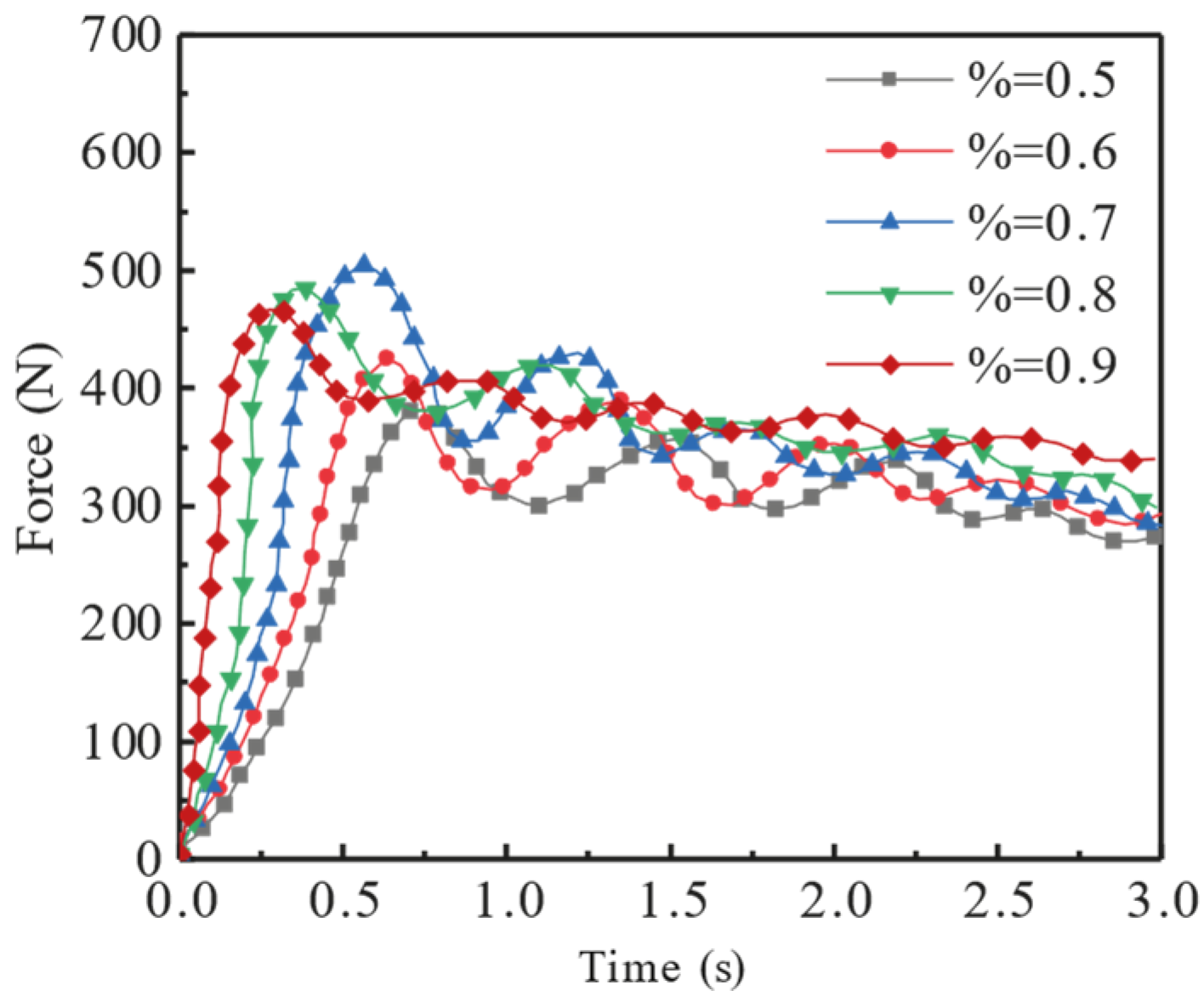
3.2.1. Influence of the TLR on the Longitudinal Impact Force

The initial driving speed of the tracked vehicle was 5 km⋅h⁻¹, while the IBD of 4 m⋅s⁻² was used for braking. The TLR was varied starting from 0.5 (to 0.9). The longitudinal impact force changed with filling ratios, as shown in Figure 7.

Figure 7 demonstrates that at the start of the braking stage, regardless of the TLR, the longitudinal impact force rapidly increased to the maximum value. The larger TLR shortened the time required to reach the maximum value. For the TLRs of 0.5, 0.6, 0.7, 0.8, and 0.9, the longitudinal impact force reached the maximum in 0.274, 0.386, 0.564, 0.634, and 0.755 s, respectively. The rapid increase in the longitudinal impact force was caused by the sharp liquid oscillation and its impact on the front wall of the tank while braking. The larger the TLR, the shorter the time needed for the longitudinal impact force to reach the peak. It also resulted in the shorter time required for attenuation to the stable value. Such behavior is attributed to the more liquid in the tank, which increases the liquid mass and its inertial force, facilitating the appearance of the maximum force.

Next, it was determined that the maximum value of longitudinal impact force was related to the liquid filling ratio. For the TLR of 0.7, the maximum longitudinal impact force was 504.5 N. According to Equation (6), the longitudinal impact force is related to the liquid quality and the degree of liquid oscillation displacement [2]. When the liquid filling ratio was 0.7, the liquid wobble increased, that is, its oscillation degree increased, and the maximum longitudinal impact force value increased.

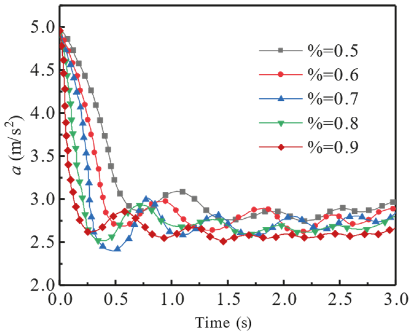
3.2.2. The Effect of TLR on the Effective Braking Deceleration

The effective braking deceleration was calculated under different TLRs, and the results are presented in Figure 7. With the increase in the TLR from 0.7 to 0.9, the time required for effective braking deceleration to decrease to the minimum value became shorter. An increase in the amount of liquid in the tank ensured that the maximum longitudinal impact force would appear more rapidly under the influence of inertia. Moreover, the minimum effective braking deceleration value appeared earlier.

When the TLR was 0.7, the effective braking deceleration was the smallest, 2.397 m⋅s⁻². This was attributed to the fact that when the TLR was 0.7, the maximum longitudinal impact force was the largest. Equation (4) indicates that the effective braking deceleration at this time was the minimum.

The fluctuation of effective braking deceleration was negatively correlated with the TLR. The liquid slosh was the most severe for the filling ratio of 0.5; when the filling ratio was 0.9, the liquid slosh was the most moderate. Its value was practically maintained at 2.5 m⋅s⁻² after 1.5 s of braking. In other words, the more fluid the tank holds, the smoother the liquid oscillations during braking.

3.2.3. Analysis of LBS for Different TLRs

The term effective braking deceleration refers to the actual deceleration of the vehicle during braking [11]. The braking efficiency is used to evaluate the change in the deceleration of the tracked vehicle, that is, its LBS. Figure 8 shows the longitudinal stability under several braking conditions with varying TLRs. When the vehicle driving speed and the IBD are fixed, the vehicle braking efficiency is greatly affected by the liquid TLR. With the increase in the TLR, the average braking deceleration rate of the tracked vehicle decreases significantly.

Figure 9 shows the longitudinal stability under braking conditions with different TLR. For the TLR of 0.7, the average braking deceleration decreased to 2.72 m⋅s⁻², while the braking efficiency decreased by 32%, resulting in the worst braking effect. Therefore, in the actual loading of hydraulic oil, the TLR of 0.7 should be avoided.

3.3. Influence of IV on Stability

Experiment group 2 was used to assess the influence of IV of the tracked vehicles on its stability.

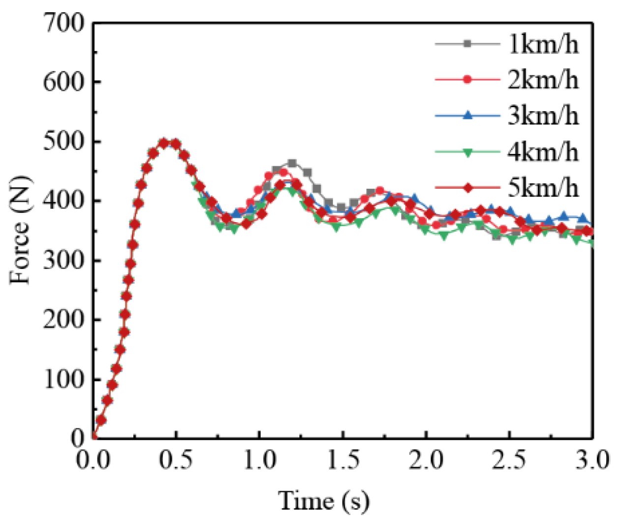
3.3.1. Influence of IV on the Longitudinal Impact Force

The IBD of the tracked vehicle was 4 m⋅s⁻², the TLR was 0.7, and the IV was varied from 1 to 5 km⋅h⁻¹. The simulation results for the longitudinal impact force obtained at different IV levels are shown in Figure 10.

At the beginning of the braking stage, the IV was varied from 1 to 5 km⋅h⁻¹. The longitudinal impact force reached the maximum value of 499.4 N at about 0.5 s. Once the longitudinal impact force reaches its maximum, its value gradually decreases and fluctuates within a given range after it falls to a certain extent. This is attributed to the backward movement of the part of the liquid due to the tank wall reaction force, thereby reducing the longitudinal impact force. Under the repeated action of the front and back walls of the tank, the longitudinal impact force shows an aperiodic attenuation trend.

Change in the IV value does not affect the time required for the longitudinal impact force to reach the maximum (~0.47 s). All five curves practically coincide in the first 0.65 s and fluctuate differently thereafter. It occurs because the IV of the liquid varies, resulting in different application times of the inertial force received by the liquid.

In general, the change in the IV shows a limited effect on the longitudinal impact force. Regardless of the IV, the liquid is statically relative to the tracked vehicle, indicating that the IV is not the factor causing the change in the longitudinal impact force of the liquid.

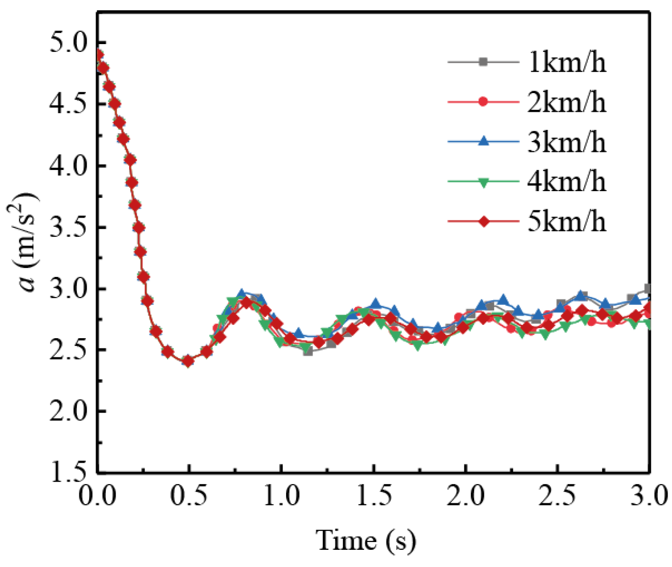
3.3.2. The Influence of IV on the Effective Braking Deceleration

The changes in the effective braking deceleration at different IVs are given in Figure 11. After the braking starts, regardless of the IV, the effective braking deceleration decreases to the minimum value of 2.41 m⋅s⁻² at around 0.5 s. Owing to the oscillation of the liquid tank and the liquid impact on the tank wall in the beginning stage of the tracked vehicle braking, the actual deceleration is less than 4 m⋅s⁻².

Once the effective braking deceleration is reduced to the minimum value of 2.41 m⋅s⁻², it starts to increase gradually. When a certain level is reached, effective braking deceleration starts to steadily fluctuate within a given value range. Its value is related to the longitudinal impact force gradually decreasing in a non-periodic trend, as the degree of liquid oscillation decreases once the longitudinal impact force reaches maximum.

Change in the IV value exhibits a limited effect on the effective braking deceleration. There are slight differences in effective braking decelerations corresponding to the five IVs; however, the fluctuation trend is the same. The fluctuation difference is caused by a small change in the longitudinal impact force.

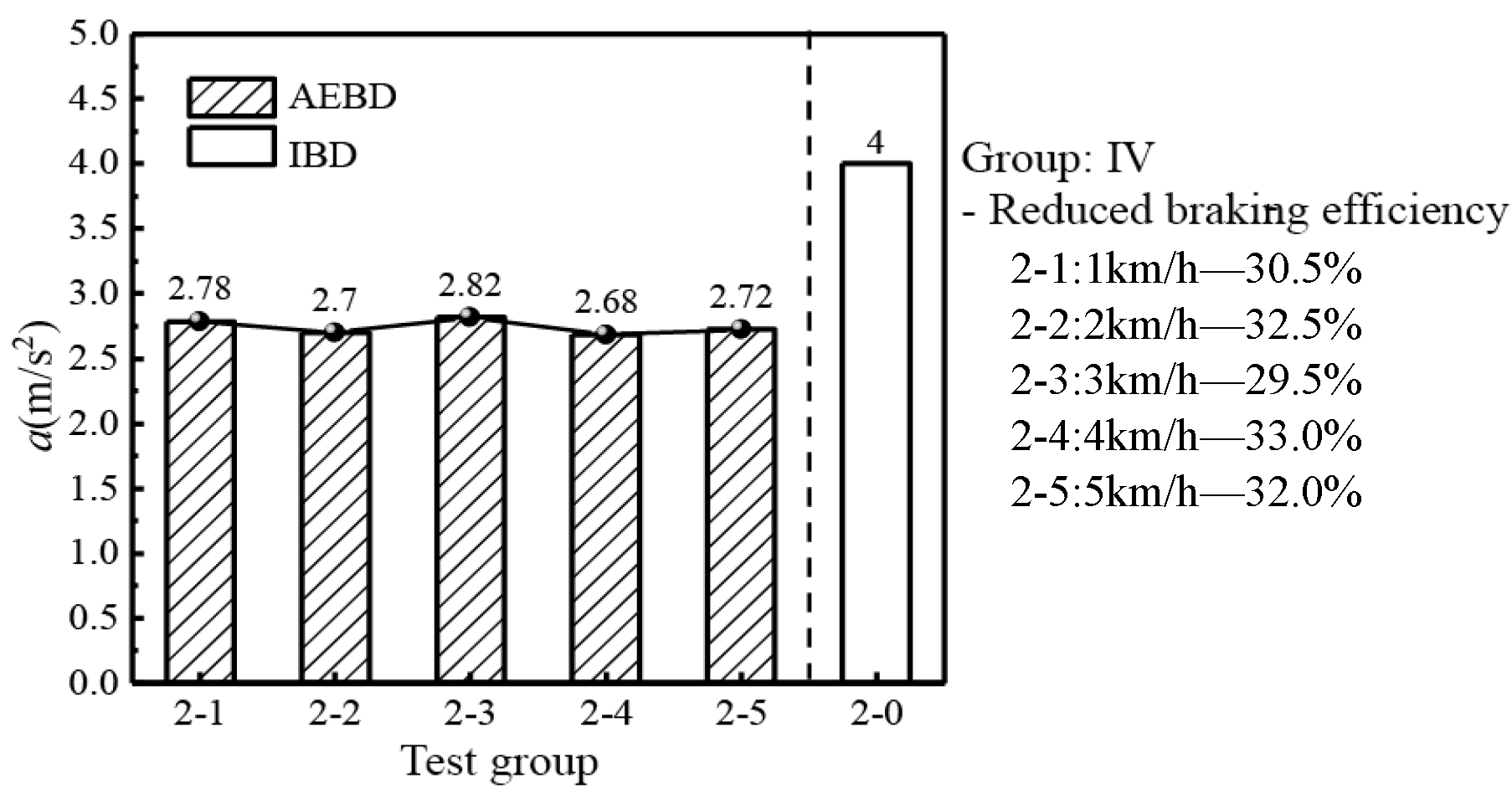
3.3.3. Analysis of the LBS at Various IVs

Based on the simulation results, the average values of effective braking deceleration (AEBD) obtained at various IVs were compared with the IBD, as shown in Figure 12. The mean effective braking decelerations of the five observed groups were similar, and the braking efficiency was reduced by about 30%. Such behavior indicates that changing only IV during the braking shows little impact on the longitudinal stability of the hydraulic tracked vehicle. However, the braking efficiency was reduced by more than 30%, thus increasing both the braking time and the braking distance. The braking distance, in turn, affects the braking safety of the tracked vehicle. Thus, the IV of the tracked vehicle exceeding 5 km⋅h⁻¹ should be avoided.

3.4. Influence of IBD on Stability

Experiment group 3 was used to observe the influence of IBD on the tracked vehicle stability.

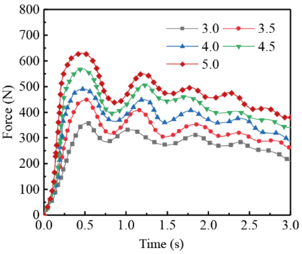
3.4.1. Influence of IBD on the Longitudinal Impact Force

The IV of the tracked vehicles was kept constant at 5 km⋅h⁻¹, the TLR was 0.7, and the deceleration speed was changed from 3 to 5 m⋅s⁻². The simulation results obtained for the longitudinal impact force at different deceleration speeds are given in Figure 13.

At the beginning of the braking stage, when the IBD changed from 3 to 5 m⋅s⁻², the longitudinal impact forces borne by the tracked vehicle all reached the peak value after around 0.5 s. Their magnitudes were 357.4, 448.7, 490.4, 568.7, and 630, corresponding to 3, 3.5, 4, 4.5, and 5 m⋅s⁻², respectively. This result can be attributed to the fact that when the tracked vehicle suddenly brakes, the liquid violently impacts the front wall of the tank, resulting in a rapid increase in the longitudinal impact force.

When the longitudinal impact force reaches its peak, its value displays an aperiodic declining trend as time prolongs. This is because, after the liquid oscillates and collides with the front wall of the liquid tank under the action of inertial force, the liquid tank wall reaction force acts on the liquid, and part of the liquid moves backward. The liquid oscillation displacement decreases, eventually leading to a gradual reduction in the liquid longitudinal impact force.

The greater the IBD, the greater the maximum longitudinal impact on the tracked vehicle. When the deceleration was 5 m⋅s⁻², the longitudinal impact force increased to 630 N at 0.5 s. This occurred since according to Equation (6), the increase in the IBD also increased the liquid deceleration, resulting in a greater longitudinal liquid impact force.

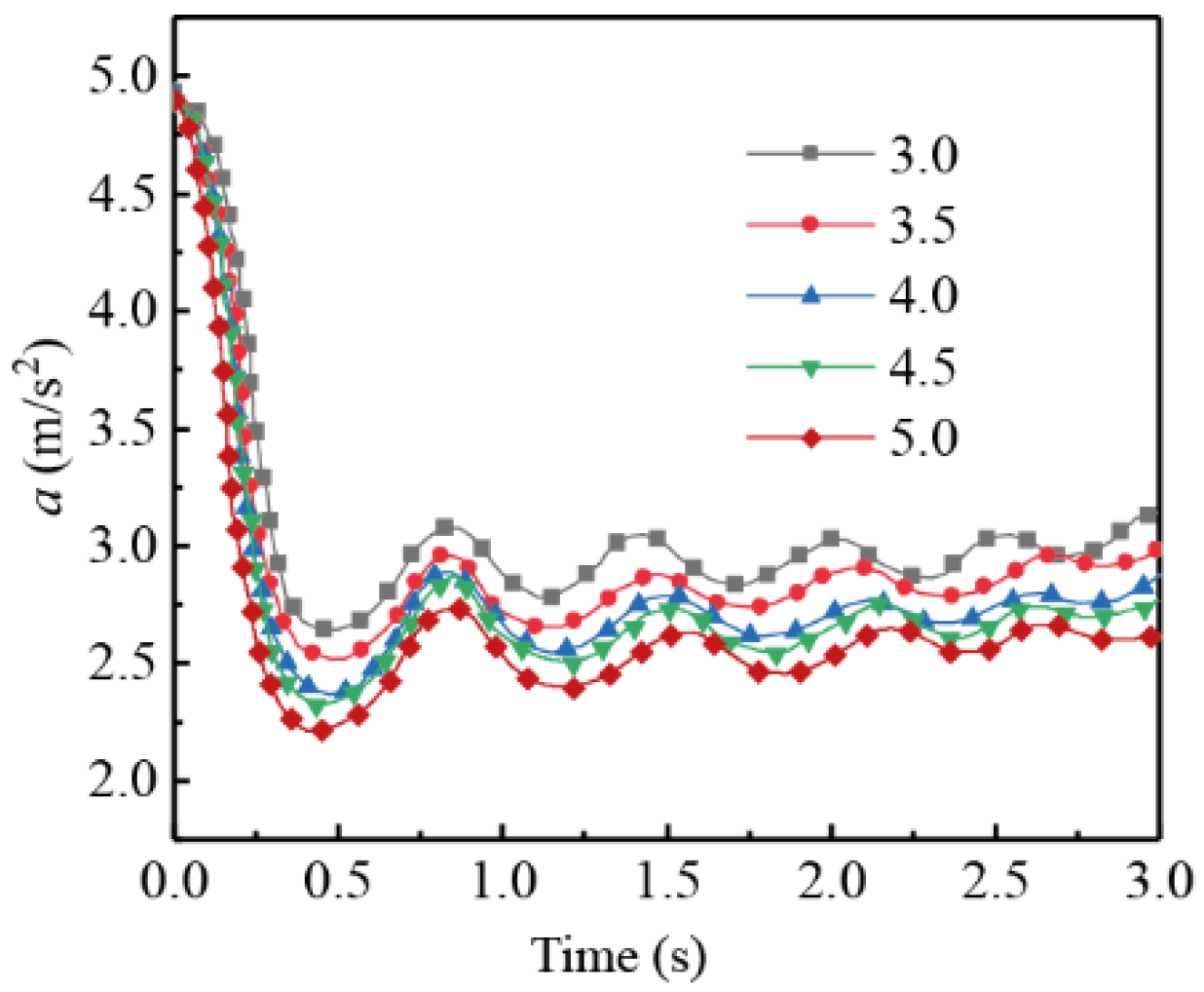
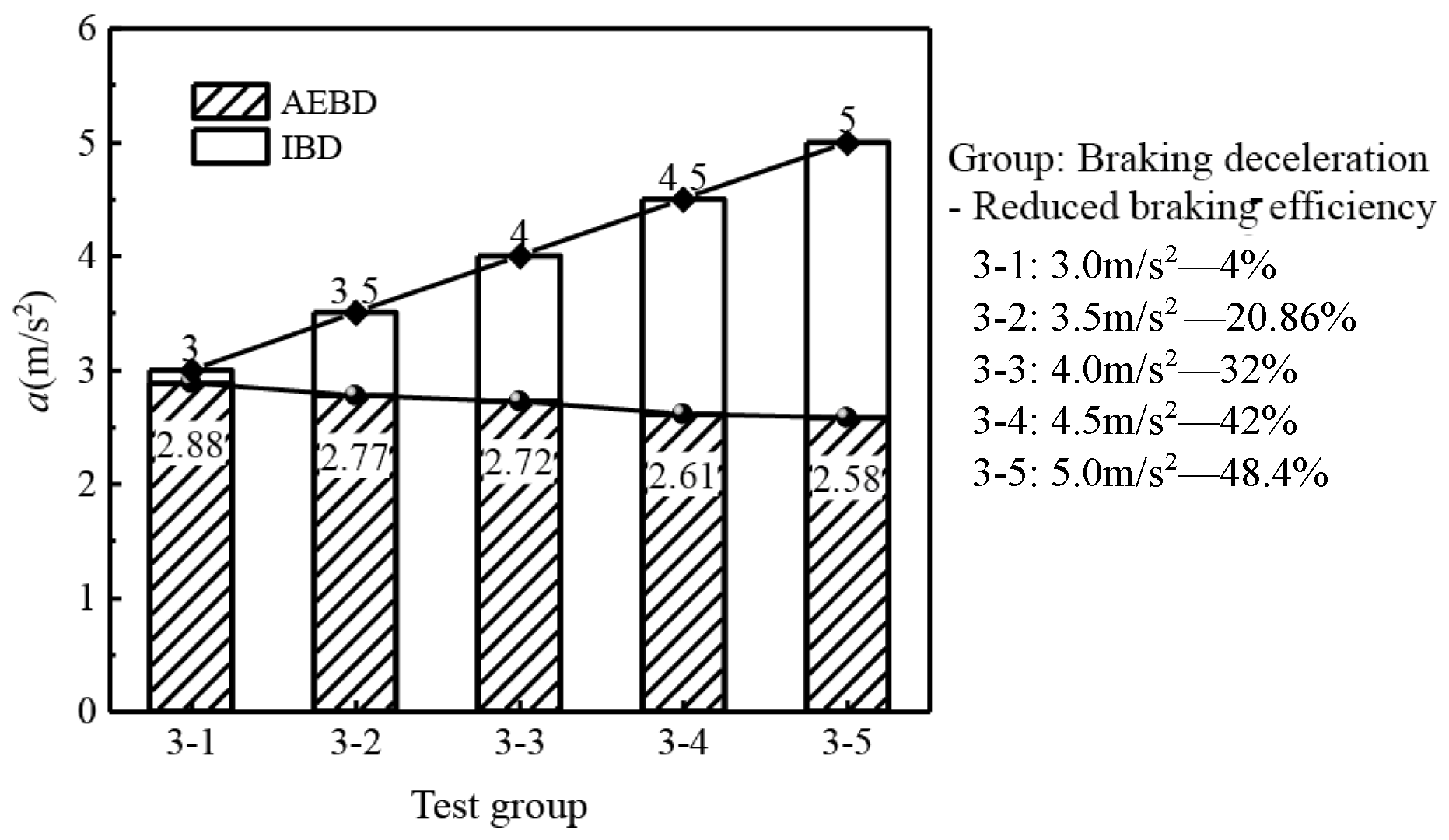
3.4.2. The Influence of IBD on the Effective Braking Deceleration

The changes in the effective braking deceleration under various IBDs are shown in Figure 14. Once the braking started, the effective braking deceleration under the five IBDs dropped to the minimum value at about 0.5 s, and the values were 2.65, 2.52, 2.37, 2.32, and 2.21 m⋅s⁻², in the descending initial deceleration order. This occurred due to the change in the longitudinal impact force of the liquid when the hydraulic tracked vehicle was braking.

The increase in IBD results in a smaller AEBD after stabilization, thus affecting the braking performance of the tracked vehicle. In the actual braking process, a larger deceleration should be avoided.

3.4.3. Analysis of LBS at Different IBDs

Figure 15 presents the comparative analysis of the AEBDs obtained for five IBDs. The braking efficiency reduction rate of tracked vehicles was positively correlated with the IBD. The larger IBD rate corresponded to a greater braking efficiency. When the IBD was increased to 5 m⋅s⁻², the braking efficiency decreased by 48.4%. Therefore, the braking time doubled and the braking distance greatly exceeded the theoretical braking distance. Such results seriously affected the braking safety of the tracked vehicle. Therefore, to ensure the safe braking of the tracked vehicle, it is necessary to avoid the use of large deceleration for emergency braking.

4. Road Experiment

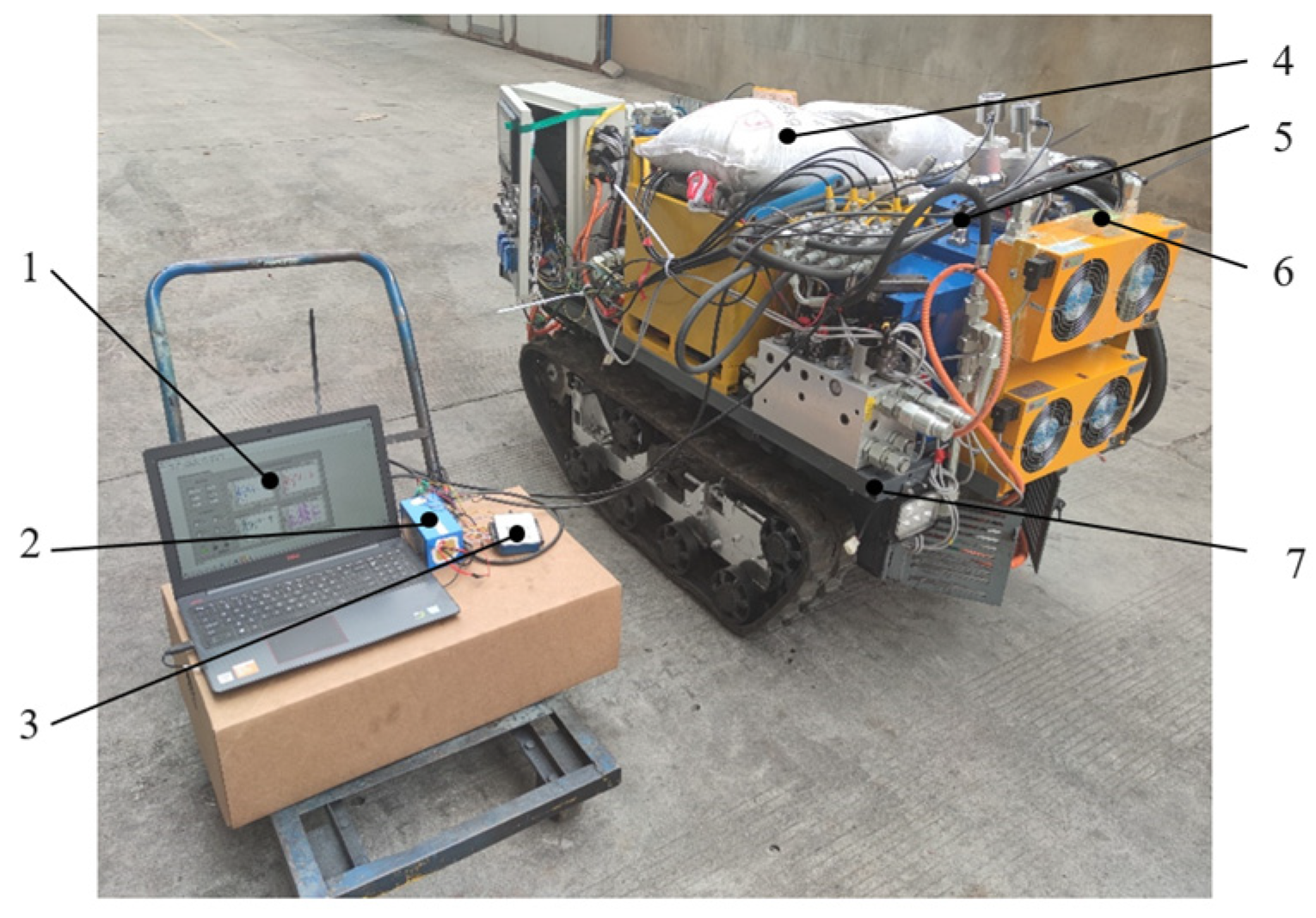
4.1. Dynamic Stability Experiment Device

Figure 16 exhibits the dynamic stability experimental device of the tracked vehicle. It was set up to experiment and verify the longitudinal stability of the tracked vehicle under braking conditions. The experimental device comprised of the physical prototype of the tracked vehicle and the data detection system.

4.2. Dynamic Stability Experiment

4.2.1. Experimental Conditions and Scheme

The experimental conditions are as follows: outdoors, 5 °C temperature, and a wind speed above 3 m⋅s⁻¹.

The experimental scheme was set according to the simulation analysis results shown above. The braking efficiency decreased by 32% or more when the TLR was 0.7. Further, the IBD speed was 4 m⋅s⁻² and the IV was 4 km⋅h⁻¹. In this case, the LBS was poor. For this reason, the LBS of tracked vehicles was tested at IVs of 1, 2, and 3 km⋅h⁻¹ under the limit conditions of critical TLR (0.7) and IBD of 4 m⋅s⁻².

The experiment was carried out on asphalt pavement with a width above 5 m and a length greater than 50 m. The acceleration sensor was fixed on the frame axle and the longitudinal acceleration a_H was measured. The angle sensor was fixed in the middle of the car rear to measure the longitudinal angular displacement θ₁. The tracked vehicle was started and was accelerated at 4 m⋅s⁻² to the IVs of 1, 2, and 3 km⋅h⁻¹ at a constant speed for 10 s. After driving at a constant speed for 20 s, the emergency braking was applied at a deceleration of 4 m⋅s⁻² until the vehicle stopped completely. The signal measured with the sensor was collected by the data acquisition card. Next, the experimental data were displayed and stored by using the software LabVIEW 2022. Three repeated experiments were conducted at each IV level.

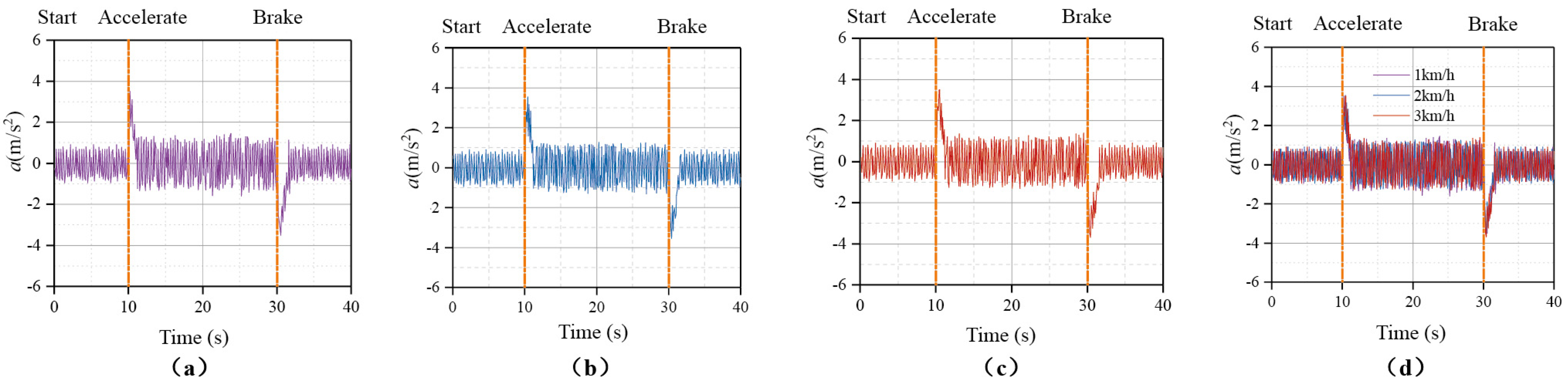
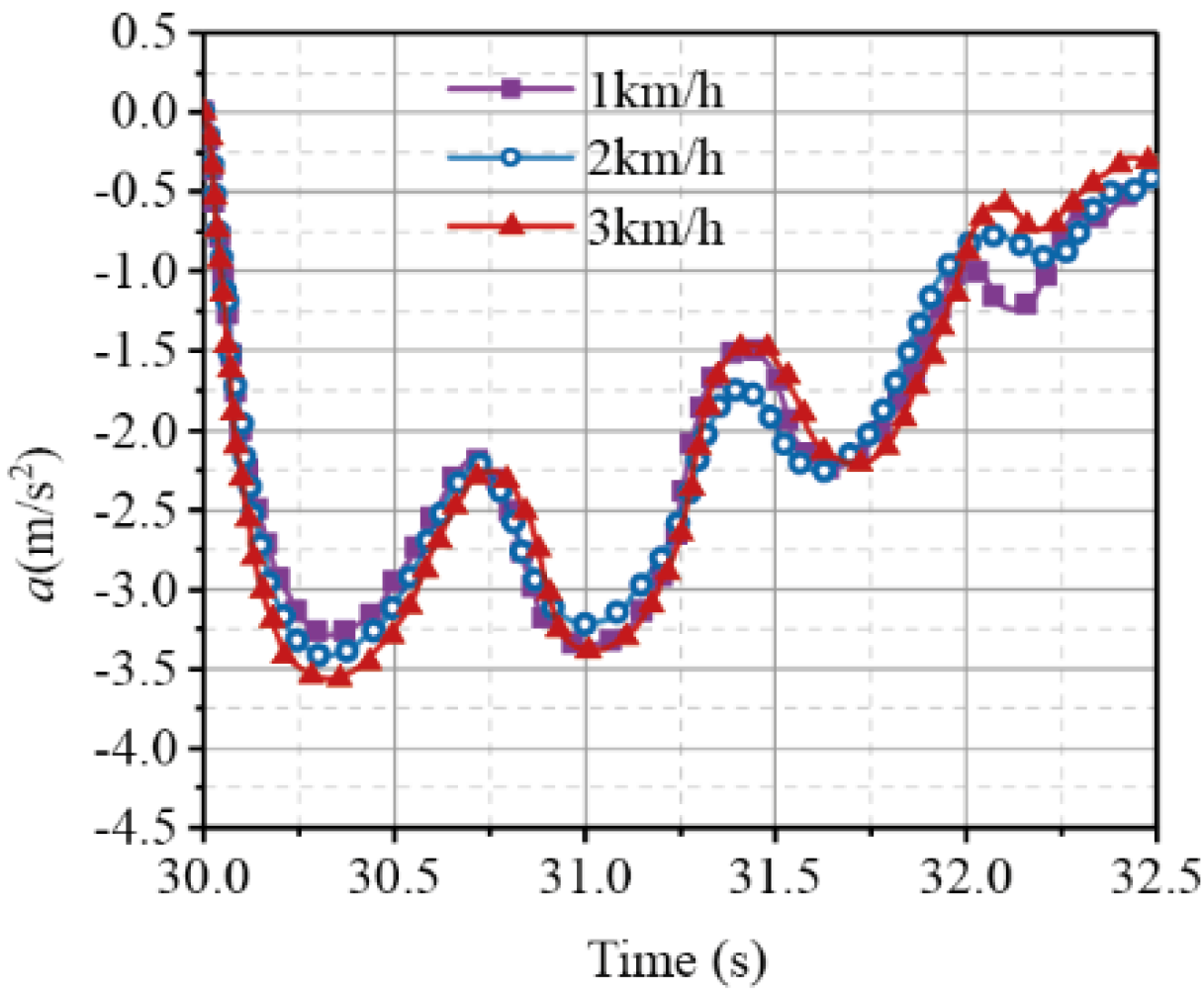
4.2.2. Influence of IV on the Effective Braking Deceleration

Experimental data for the effective braking deceleration were obtained corresponding to the start, acceleration, movement, and braking of the tracked vehicle at the IVs of 1, 2, and 3 km⋅h⁻¹, respectively, and the corresponding data are shown in Figure 17.

Change trends in effective braking deceleration values during starting, accelerating, walking, and emergency braking at different IVs were practically the same. These results indicate that when the TLR and braking deceleration are fixed, change in the movement speed shows a limited effect on the effective braking deceleration.

The effective braking deceleration of the tracked vehicle shows a sudden change after 10 s of acceleration and 30 s of braking. The remaining stages display an approximately periodic fluctuation, which increases in magnitude between 10 and 30 s. This is due to the sudden acceleration or braking of the vehicle, which causes the forced vibration of its motor, reducer, and pump, among other parts. As such, it intensifies the degree of oscillation of the liquid and the entire body: therefore, the effective braking deceleration fluctuates within a certain range. Furthermore, the higher the speed, the more obvious the superposition effect of forced vibration, and the greater the fluctuation of longitudinal acceleration.

The experimental data obtained for braking conditions at three IVs were filtered and amplified, as shown in Figure 18.

Figure 18 shows that after the braking starts, regardless of the value of IV, the longitudinal acceleration decreases to its minimum value at about 30.3 s. When the tracked vehicle is braking, the liquid oscillation and the impact on the tank wall reduce the vehicle braking performance. It results in the actual effective braking deceleration of less than 4 m⋅s⁻².

Once the effective braking deceleration was reduced to the minimum, its value gradually increased; its absolute value decreased more significantly compared to that shown in Figure 14. This was due to the forced vibration of the motor, gearbox, and pump, in addition to other components, which was caused by sudden acceleration or braking, and intensified the degree of liquid oscillation. Compared to Figure 13, the longitudinal force of the liquid was greater and the effective braking deceleration was reduced to a greater extent.

The variation trend in the effective braking deceleration obtained in the experiment was found to be consistent with the simulation results. However, the time required to decrease it to the minimum value was shorter.

4.2.3. Influence of the IV on the Longitudinal Angular Displacement

Angle sensors were used to measure the longitudinal angular displacement θ₁ of the tracked vehicle when the traveling speed was 1, 2, and 3 km⋅h⁻¹, respectively, and the results are shown in Figure 19.

The overall change trends of longitudinal angular displacement of tracked vehicles were nearly identical during starting, accelerating, walking at different IVs, and braking. This shows that when accelerating and braking with the same acceleration, change in only IV shows an identical effect on the longitudinal driving stability of the hydraulic tracked vehicle.

When the tracked vehicle suddenly accelerated at 10 s, its front appeared to warp with a maximum warp angle of about 4°. The reason for such behavior is that the tracked vehicle experiment has a rear-wheel drive. When the tracked vehicle accelerates, the drive wheel rotates forward and the body is subjected to the force in the opposite direction. This causes the ground pressure of the track front wheel to be lower compared to that under the stationary case; thus, the ground pressure of the rear wheel is greater than that of the front wheel when it is stationary. When the ground pressure of the front wheel is zero, the head tilts. The maximum tilt angle is θ_1max ≤ 5°. The stability check by the moment method shows that it meets the stability requirement.

When the tracked vehicle performed the emergency parking braking at the 30 s point, the vehicle rear was cocked, and the maximum tilt angle was 4°. In the braking moment of the tracked vehicle, the driving wheel locks rapidly. Under the action of inertial force, the rear wheel of the track is warped when the front wheel is the fulcrum. The maximum tilt angle is θ_1max ≤ 5°, meeting the stability requirements.

5. Conclusions

The tracked vehicle works at a complex and narrow disaster site, and thus it is important and innovative to investigate its braking stability, which was evaluated in this study. Further, the fluid–structure coupling analysis of oil, liquid tank, and track vehicle was carried out when analyzing the longitudinal stability of tracked vehicle.

• The braking dynamics model of the lightweight mini-track vehicle was established. According to the model, the effective braking speed reduction was positively correlated with the total mass of the tracked vehicle when the tracked vehicle was impacted by the liquid tank during running. Furthermore, it was negatively correlated with the longitudinal impact force of the liquid oscillation. In other words, the smaller the tracked vehicle mass, the greater the longitudinal impact force. Moreover, smaller vehicle mass also corresponds to a smaller effective braking deceleration, inferior longitudinal stability, and longer braking time.
• Based on the fluid motion equation applied to the liquid tank and the theoretical model of longitudinal impact force, the influences of the TLR, IV, and IBD on the longitudinal stability of the observed vehicle were analyzed. It is noteworthy that the control variable method and the fluid simulation software FLUENT 2023 were used. The results show that the TLR significantly impacted the braking efficiency of the tracked vehicle. The braking effect was the weakest for the filling ratio of 0.7, and the braking efficiency decreased by 32% compared to its initial value. Changing only the IV exhibited a limited effect on the longitudinal stability of the tracked vehicle. Further, the braking efficiency was also reduced by about 30% compared with the IBD. When the IBD was changed, the braking efficiency reduction rate was positively correlated with it. Finally, when the IBD speed was increased to 5 m⋅s⁻², the braking efficiency decreased by more than 48%.
• The dynamic stability experimental platform of the lightweight mini-tracked vehicle was built. The limit conditions of the TLR of 0.7 and effective braking deceleration of 4 m⋅s⁻² were selected for the experimental case. The longitudinal stability of the tracked vehicle during the starting, accelerating, walking, and emergency braking at IVs of 1, 2, and 3 km⋅h⁻¹ was evaluated. Based on the results, the following conclusions were drawn: when the TLR and effective braking deceleration were constant, the change in the IV exhibited a limited effect on the effective braking deceleration. Compared to the simulation results, the AEBD obtained in the experiment was smaller. This was due to the sudden acceleration or braking of the tracked vehicle during the road experiment, which caused forced vibration of its motor, gearbox, and pump, among other components. The forced vibration led to a further increase in the longitudinal force of the liquid, thus reducing effective braking deceleration.
• When the tracked vehicle accelerated and braked under extreme conditions, the front and rear tilt angles were approximately 4°. This value is below 5°, which indicates that the stability requirements are met.
• Owing to time and resource constraints, only the longitudinal stability of the tracked vehicle during the braking was studied. However, the road conditions of the tracked vehicle during the rescue were harsh. Therefore, it might be valuable to systematically examine the lateral rollover stability and longitudinal stability of the tracked vehicle under various working conditions.

References

1. Wan, Y.; Zhao, W.Q.; Zong, C.F.; Zheng, H.Y.; Li, Z.Y. Modelling and Analysis of the Influences of Various Liquid Sloshing Characteristics on Tank Truck Dynamics. Int. J. Heavy Veh. Syst. 2019, 26, 463–493. [Google Scholar] [CrossRef]
2. Shi, H.L.; Wang, L.; Nicolsen, B.; Shabana, A.A. Integration of Geometry and Analysis for the Study of Liquid Sloshing in Railroad Vehicle Dynamics. Proc. Inst. Mech. Eng. Part K J. Multi-Body Dyn. 2017, 231, 608–629. [Google Scholar] [CrossRef]
3. Wu, W.J.; Gao, C.N.; Yue, B.Z.; Deng, M.L. Experimental Study and Dynamic Characteristic Analysis of Nonlinear Steady State Sloshing of Liquid in a Cylindrical Tank. J. Astronaut. 2021, 42, 1078–1089. [Google Scholar]
4. Li, X. Research on the Longitudinal Stability of Tank Vehicles on Liquid Sloshing. Master’s Thesis, Jilin University, Changchun, China, 2016; pp. 10–12. [Google Scholar]
5. Azadi, S.; Jafari, A.; Samadian, M. Effect of Parameters on Roll Dynamic Response of an Articulated Vehicle Carrying Liquids. J. Mech. Sci. Technol. 2020, 28, 837–848. [Google Scholar] [CrossRef]
6. Zhou, F.X. Study on Handling Dynamics and Stability of Heavy-duty Vehicles with Storage Tank. Master’s Thesis, Guangxi University Science Technology, Liuzhou, China, 2020; pp. 33–36. [Google Scholar]
7. Wang, L. Research on Anti-Rollover Stability of Tank Semi-Trailer Considering Vehicle-Liquid Coupling. Master’s Thesis, Harbin Institute Technology, Harbin, China, 2021; pp. 31–35. [Google Scholar]
8. Zheng, X.L.; Li, X.S.; Ren, Y.Y. Rollover Stability Analysis of Tank Vehicle Impacted by Transient Liquid Sloshing. J. Jilin Univ. (Eng. Technol. Ed.) 2014, 44, 61–64. [Google Scholar]
9. Li, H. Fluid-Structure Coupling Stress Analysis of Tank for Tank Truck and Study of Internal Fluid Sloshing. Master’s Thesis, Northeastern University, Shenyang, China, 2018; pp. 42–46. [Google Scholar]
10. Chen, J.M. Analysis on Characteristics of Liquid Sloshing in Automobile Fuel Tank under Multiple Operating Condition. Master’s Thesis, Wuhan University of Technology, Wuhan, China, 2019; pp. 24–41. [Google Scholar]
11. Feng, C.Q. Study on Longitudinal Sloshing of Liquid Tank Car and Vehicle Dynamics Model. Master’s Thesis, Kunming University of Science and Technology, Kunming, China, 2020; pp. 67–82. [Google Scholar]
12. Zhang, J.W.; Wang, W.Y.; Peng, Y.H.; Li, X.D. A Study on Turning-braking Stability of a Tanker. Automot. Eng. 2019, 2, 118–123. [Google Scholar]
13. Yu, Z.S. Automobile Theory, 6th ed.; China Machine Press: Beijing, China, 2018. [Google Scholar]
14. Ranganathan, R.; Rakheja, S.; Sankar, S. Steady Turning Stability of Partially Filled Tank Vehicles with Arbitrary Tank Geometry. J. Dyn. Sys., Meas. Control 2019, 111, 481–489. [Google Scholar] [CrossRef]
15. Zhang, E.H.; He, R.; Su, W.D. Numerical Analysis of Oil Liquid Sloshing Characteristics in fuel tank with different baffle structure. J. Jilin Univ. (Eng. Technol. Ed.) 2021, 1, 83–95. [Google Scholar]
Figure 1. The 3D model of the chassis of the tracked vehicle: 1. Guide wheel; 2. tension buffer device; 3. support heavy wheel; 4. belt support wheel; 5. rack; 6. track; 7. driving wheel; 8. driving motor.
Applsci 14 07780 g001
Figure 2. Layout of each component on the chassis of the tracked vehicle: 1. Lighting; 2. valve block; 3. battery; 4. carriage; 5. high-pressure pump; 6. low-pressure pump; 7. electric control box; 8. cooler; 9. liquid tank; 10. water tank; 11. reducer box; 12. motor; 13. motor controller.
Applsci 14 07780 g002
Figure 3. Braking force diagram of the tracked vehicle.
Applsci 14 07780 g003
Figure 4. Tank model and boundary conditions.
Applsci 14 07780 g004
Figure 5. Relationship between turbulent dissipated energy and mesh size.
Applsci 14 07780 g005
Figure 6. Grid division.
Applsci 14 07780 g006
Figure 7. Simulation results for the longitudinal impact force.
Applsci 14 07780 g007
Figure 8. Curves for the change in the effective braking deceleration.
Applsci 14 07780 g008
Figure 9. Longitudinal stability diagram.
Applsci 14 07780 g009
Figure 10. Simulation results obtained for the longitudinal impact force.
Applsci 14 07780 g010
Figure 11. Curves showing changes in the effective braking deceleration.
Applsci 14 07780 g011
Figure 12. Evaluation diagram of the longitudinal stability.
Applsci 14 07780 g012
Figure 13. Simulation results of longitudinal impact force.
Applsci 14 07780 g013
Figure 14. Changes in the effective braking deceleration curve.
Applsci 14 07780 g014
Figure 15. Evaluation of the longitudinal stability.
Applsci 14 07780 g015
Figure 16. Dynamic stability test platform of tracked vehicle: 1. Upper computer; 2. the 24 V power supply; 3. data acquisition card; 4. the 200 kg weight; 5. three-axis acceleration sensor; 6. angular displacement sensor; 7. physical prototype of the tracked vehicle.
Applsci 14 07780 g016
Figure 17. Experimental data obtained for effective braking deceleration during starting, accelerating, walking, and braking of a tracked vehicle: (a) IV 1 km⋅h−1; (b) IV 2 km⋅h−1; (c) IV 3 km⋅h−1; and (d) comparison of each IV condition.
Applsci 14 07780 g017
Figure 18. Locally enlarged data of braking conditions at different speeds.
Applsci 14 07780 g018
Figure 19. Experimental data obtained for longitudinal angular displacement of the tracked vehicle during starting, accelerating, walking, and braking: (a) IV 1 km⋅h−1; (b) IV 2 km⋅h−1; (c) IV 3 km⋅h−1; and (d) comparison of each IV condition.
Applsci 14 07780 g019