Nonlinear Modeling and Transient Stability Analysis of Grid-Connected Voltage Source Converters during Asymmetric Faults Considering Multiple Control Loop Coupling

Abstract

As large-scale renewable energy sources are increasingly integrated into AC grids via voltage source converters (VSCs), the transient synchronization stability of phase-locked loop (PLL)-based VSCs during fault ride-through is gaining more attention. Most existing studies assume that the positive and negative sequence separation and current control dynamics are much faster than the PLL dynamics, thereby neglecting their impact on the transient synchronization stability of the system. However, when the PLL bandwidth is relatively large, ignoring the positive and negative sequence separation and current control dynamics may result in incorrect stability assessments. To address this issue, this paper first considers the multiple control loop coupling, including positive and negative sequence separation, current control, and PLL, to construct a full-order nonlinear mathematical model of the VSC grid-connected system under asymmetric fault conditions. Based on this, the phase trajectory method is employed to analyze the transient synchronization stability of the system. Additionally, this full-order mathematical model is used to determine the PLL bandwidth boundary beyond which the effects of positive and negative sequence separation and current control dynamics cannot be neglected. Finally, PSCAD/EMTDC simulation results validate the effectiveness of the theoretical analysis presented in this paper.

1. Introduction

With the advantages of a simple structure for active and reactive power decoupling control and easy current limiting ability, control strategies based on the d-q rotating coordinate system and phase-locked loop (PLL) synchronization have been widely used in grid-feeding VSCs [1]. At present, the majority of grid-feeding VSCs still use PLL to achieve synchronization [2]. However, numerous theoretical studies and real-world engineering cases have indicated that grid-feeding converters with PLL are exposed to the risk of transient synchronization instability, particularly under grid faults [3,4]. Thus, it is essential to investigate the transient stability of grid-connected VSC systems under fault conditions.

Current research predominantly focuses on the transient synchronization stability of VSC grid-connected systems under symmetric fault conditions. References [5,6] point out the mathematical similarity between PLL dynamic models and synchronous machine rotor motion equations, using the equal area criterion to reveal the transient synchronization instability mechanism of VSC grid-connected systems. References [7,8,9,10] and [11,12,13] employ the phase trajectory method, inverse trajectory method, and direct method, respectively, to quantitatively analyze the transient synchronization stability of VSC grid-connected systems. Additionally, references [14,15,16] analyze the impact of dynamic interactions within the current inner loop on the transient synchronization stability of the system under fault conditions. However, these studies primarily address the transient synchronization stability of VSC grid-connected systems under symmetric grid faults. In practice, asymmetric faults are more common. As reported in [17], PLL synchronization instability during asymmetrical line-to-line and single line-to-ground faults in California in 2016 led to the disconnection of 700 MW in a large photovoltaic power plant. Thus, analyzing the transient synchronization stability of grid-connected VSCs under asymmetric faults is equally important.

Existing studies on synchronization stability under asymmetric faults mainly investigate three aspects: the existence of equilibrium points during asymmetric faults, the stability of these equilibrium points, and the system’s ability to return to equilibrium after a fault. For the existence of equilibrium points, reference [18,19,20] establishes a reduced-order dynamic model suitable for analyzing PLL synchronization stability under asymmetric faults and derives static synchronization stability criteria to ensure the existence of equilibrium points post-fault. Clearly, if the system lacks equilibrium points during a fault, it will inevitably experience transient instability. However, the existence of equilibrium points during a fault does not guarantee transient stability, as it also depends on the system’s dynamic processes.

Regarding the small-signal stability analysis of equilibrium points, reference [21] constructs a complex frequency domain impedance model of the VSC grid-connected system under asymmetric grid faults, using the generalized Nyquist criterion to analyze small-signal stability during asymmetric faults. Reference [22] develops a high-order state-space analysis model under asymmetric faults and uses eigenvalue analysis to study the impact of positive and negative sequence currents on the small-signal stability of the VSC grid connection. It is important to note that references [21,22] base their analysis on linearized models, which cannot fully describe the transient synchronization process under large disturbances like asymmetric grid faults, where the post-fault operating point deviates significantly from the pre-fault steady-state operating point. In such cases, the nonlinear characteristics of the VSC grid connection must be considered, and transient stability analysis methods are required.

For transient synchronization stability analysis, references [23,24] ignore the coupling between positive and negative sequence dynamics, separately analyzing the transient synchronization stability of positive and negative sequence systems. However, under asymmetric faults, especially when the fault point is near the grid connection point, the coupling between positive and negative sequence dynamics cannot be ignored. To address this, reference [25] constructs a mathematical model considering the coupling of positive and negative sequences and uses the TS method to quantitatively analyze the system’s transient synchronization stability. However, most of these studies assume that PLL dynamics are much slower than positive and negative sequence separation and current control dynamics. In reality, if the PLL bandwidth is not particularly small, the transient synchronization stability analysis models considering only PLL dynamics, as proposed in references [23,24,25], may lead to incorrect stability assessment results.

Therefore, it is necessary to analyze the transient synchronization stability of grid-connected VSC systems considering the coupling effects of multiple control loops, including positive and negative sequence separation, current control, and PLL control. However, the existing literature seldom addresses this aspect. More importantly, during transient synchronization stability analysis, it is not clear under what conditions a nonlinear mathematical model considering only PLL dynamics can be used to analyze the system’s transient synchronization stability. This paper aims to address these questions as a primary research objective.

The main contributions of this paper are summarized as follows:

(1)

Considering the coupling of multiple control loops, including positive and negative sequence separation, current control, and PLL control, a full-order nonlinear mathematical model of the VSC grid-connected system under asymmetric fault conditions is constructed. The phase trajectory method is used to analyze the system’s transient synchronization stability under asymmetric faults.

(2)

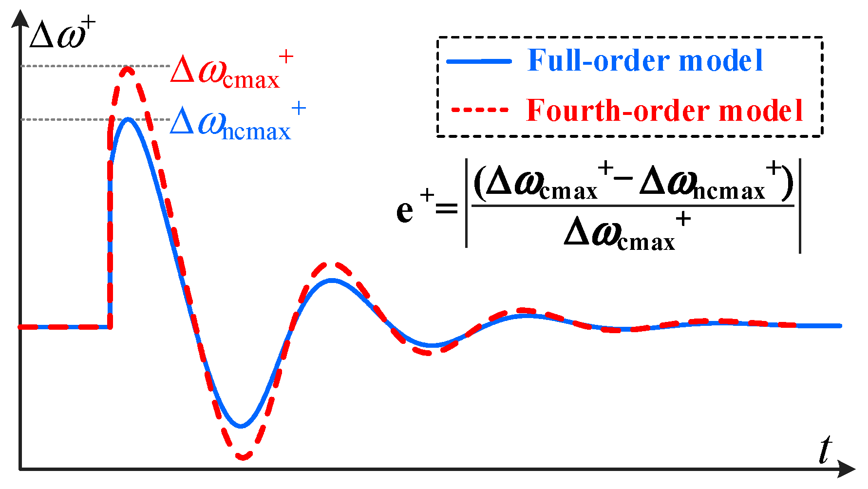
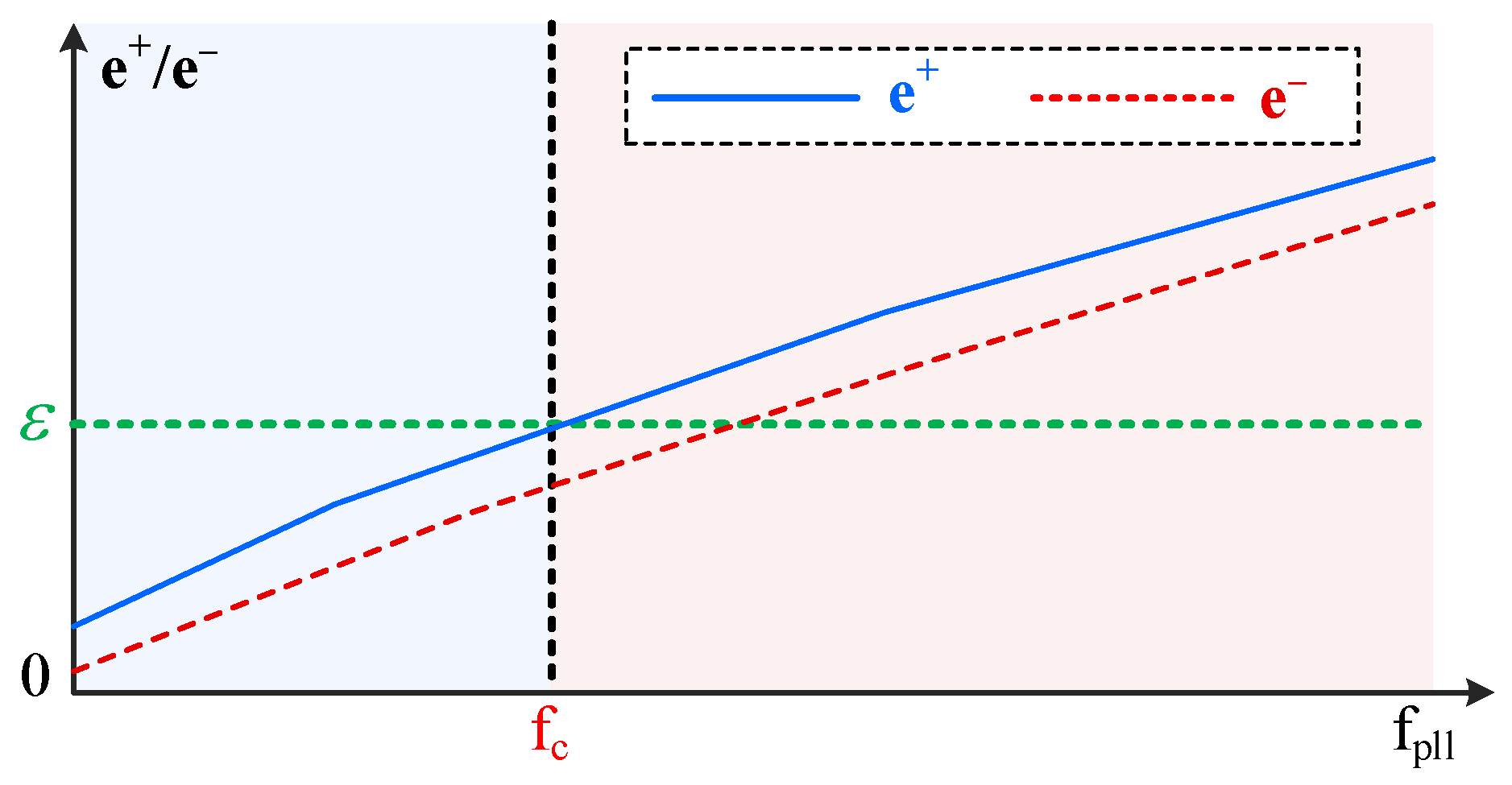
Based on the full-order mathematical model established in this paper, numerical methods are used to analyze the PLL bandwidth threshold within which the impacts of positive and negative sequence separation and current control dynamics can be ignored. This provides a theoretical basis for the design of control parameters for grid-connected converters.

2. System Description

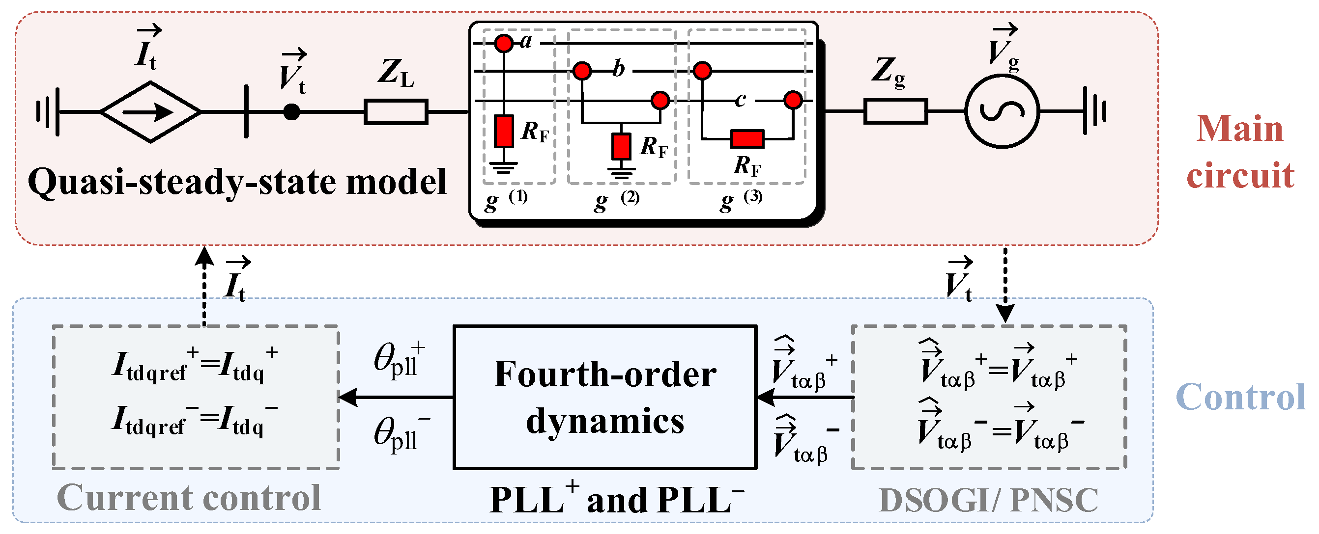
2.1. System Overview

The topology and control of the system are presented in Figure 1. The VSC is connected to the weak grid through a Delta-wye (Dy) grounded step-up transformer. The impedance of the transformer is much less than that of the line impedance; thus, the transformer is considered as an ideal transformer in this paper.

In Figure 1, e_abc, v_tabc, v_Fabc, and v_gabc are the abc three-phase components of VSC output voltage, low-voltage-side PCC voltage, fault point voltage, and infinite-bus voltage, respectively. i_tabc denotes the abc three-phase component of the current injected by the VSC into the grid. The equivalent impedances from the point of common coupling (PCC) to fault location and from fault location to infinite-bus are denoted as Z_L and Z_g, respectively. Notably, different asymmetric fault types are denoted by g⁽ⁿ⁾, where g⁽¹⁾, g⁽²⁾, and g⁽³⁾ denote single line-to-ground (SLG), double line-to-ground (DLG), and line-to-line (LL) faults, respectively.

The control strategy of VSC comprises dual second-order generalized integrator- positive/negative-sequence calculator (DSOGI/PNSC), the positive and negative sequences PLL (PLL⁺ and PLL⁻), and proportional resonant (PR)-based dual-sequence current control in stationary reference frames.

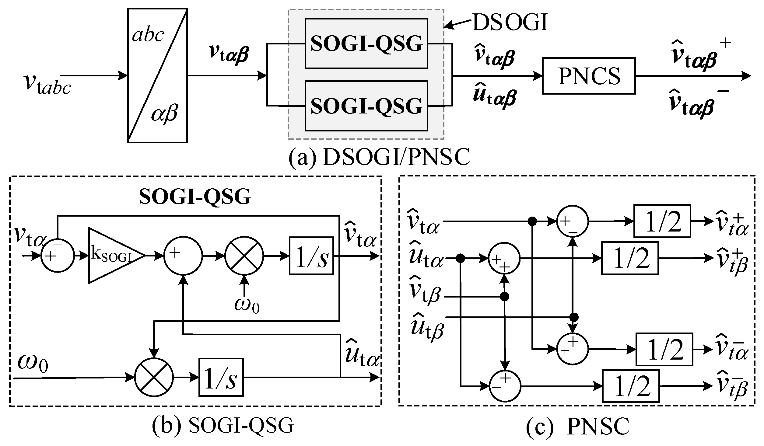
2.2. DSOGI/PNSC Control Structure

The control structure of DSOGI/PNSC is shown in Figure 2, in which DSOGI contains two second-order generalized integrator–quadrature signals generators (SOGI–QSGs). The DSOGI enables quadrature phase division and harmonic suppression of the voltage at the PCC. The PNSC can obtain the PS and NS voltage components at the PCC in the αβ coordinate system based on the output of DSOGI.

2.3. PLL⁺ and PLL⁻ Control Structure

Figure 3 gives the control structure of PLL⁺ and PLL⁻. The PLL⁺ and PLL⁻ take positive and negative sequence voltages of PCC as inputs, respectively, and output the positive and negative sequence angular frequency ω_pll⁺, ω_pll⁻, and phase angle θ_pll⁺, θ_pll⁻.

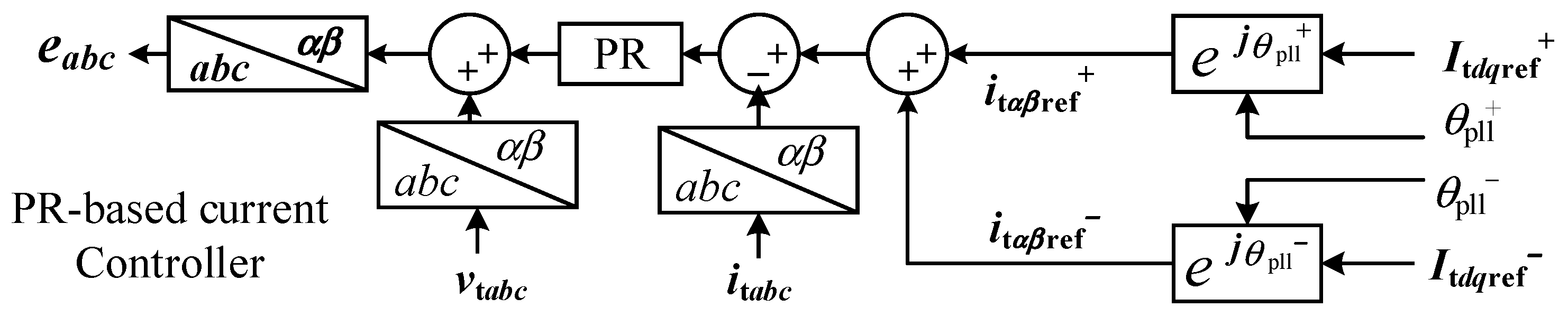
2.4. PR-Based Dual-Sequence Current Control

The control structure of PR-based dual-sequence current control is illustrated in Figure 4. The PR-based current control regulates the converter-side currents, enabling the VSC dual-sequence injection current to follow the PS and NS current reference values I_tdref⁺, I_tqref⁺, and I_tdref⁻, I_tqref⁻. Note that the PN sequence current references are directly specified when the grid-connected VSC system is exposed to asymmetric grid faults.

2.5. Fourth-Order Model Considering Only Phase-Locked Loop Dynamics

Ref. [25] considers the PLL bandwidth that is significantly smaller than the bandwidth of the LC filter and AC network transient, PR-based current control dynamics, and the DSOGI//PNSC dynamics. Therefore, the impact of the LC filter, AC network transients, PR-based current control dynamics, and DSOGI/PNSC dynamics on the transient characteristics of the system is much smaller compared to the PLL dynamics. As a result, Ref. [25] neglects the effects of the LC filter, AC network transients, PR-based current control dynamics, and DSOGI/PNSC dynamics, leading to the equivalent circuit shown in Figure 5. Then, a fourth-order synchronization model that only considers PLL dynamics is constructed to analyze the transient synchronization stability of the system during asymmetric faults. The detailed mathematical expressions and derivation process of the fourth-order model can be found in [25] and are not provided in this paper.

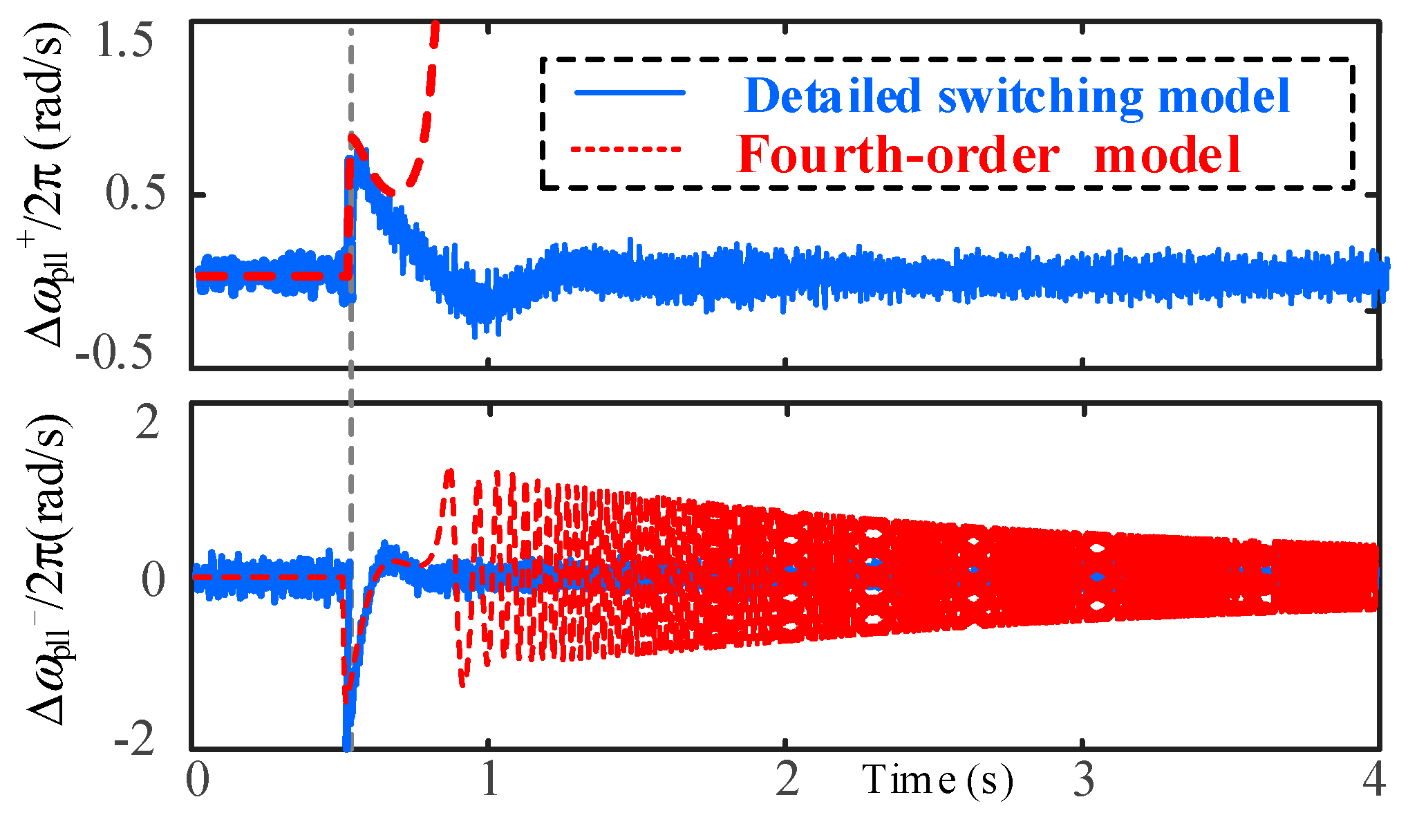
2.6. The Necessity of Considering Multiple Control Coupling

In certain special cases, the bandwidth of the PLL cannot be designed to be too small. In such cases, a model only considering PLL dynamics may not accurately capture the system’s dynamics. To illustrate this, consider a double line-to-ground fault, PS and NS current reference values I_tdref⁺, I_tqref⁺, and I_tdref⁻, I_tqref⁻ are selected as 0.4, 0.5, and 0, 0.5, respectively, referred to as Case 1. Figure 6 compares the simulation results of the fourth-order model, which only considers PLL dynamics, with those of the detailed electromagnetic transient switching model. System parameters are listed in Appendix A,

Table A1. System parameters on the low-voltage side.

System	Parameter Name	Value
Base values	Base value of power	50 kW
	Base value of AC voltage	400 V
	Base value of frequency	50 Hz
Hardware parameters	Switching frequency	10 kHz
	LC filter Lf/Cf	0.1/0.04 pu
	XL/RL	0.5/0.05 pu
	Xg/Rg	0.4/0.04 pu
	Ground resistance RF	4.5 × 10−6 pu
	Itd,0+/Itq,0+/Vg	0.9 pu/0.4 pu/1 pu
	Maximum current Im	1 pu
Control parameters	PLL PI parameters kp/ki	100/2000
	Gain of SOGI unit kSOGI	1.414
	PR parameters kpi/kri/ωc	0.5/5/6.5

. As shown in Figure 6, the fourth-order model (dashed line), which only considers PLL dynamics, indicates transient instability during asymmetric faults. However, the detailed electromagnetic transient switching model (solid line) shows that transient synchronization instability will occur.

This result in Figure 6 demonstrates that the fourth-order model, which considers only PLL dynamics, fails to accurately reflect the dynamic characteristics of the system when the PLL bandwidth is relatively large. The erroneous conclusion from the fourth-order model arises because, with a larger PLL bandwidth, the transient synchronization process of the VSC is no longer solely dominated by the PLL dynamics. It is also influenced by the LC filter and AC network transient, PR-based current control dynamics, and the DSOGI//PNSC dynamics. Ignoring the coupling effects between multiple control loops will inevitably lead to incorrect analysis results.

Therefore, it is crucial to consider the detailed nonlinear model of the system to study the transient stability considering the coupling of multiple control loops. This is the main motivation for this paper.

3. Detailed Nonlinear Modeling of Grid-Connected VSCs during Asymmetric Faults

This section develops a detailed nonlinear model of grid-connected VSCs during asymmetric faults, considering the LC filter and AC network transient, PR-based current control dynamics, DSOGI dynamics, and PLL dynamics. First, the coordinate system used for modeling in this paper is given in Section 3.1. Then, in Section 3.2, the mathematical model of the main circuit is built. Next, the mathematical model of the control is constructed in Section 3.3. Finally, in Section 3.4, the complete nonlinear mathematical model of the system during asymmetric fault is obtained.

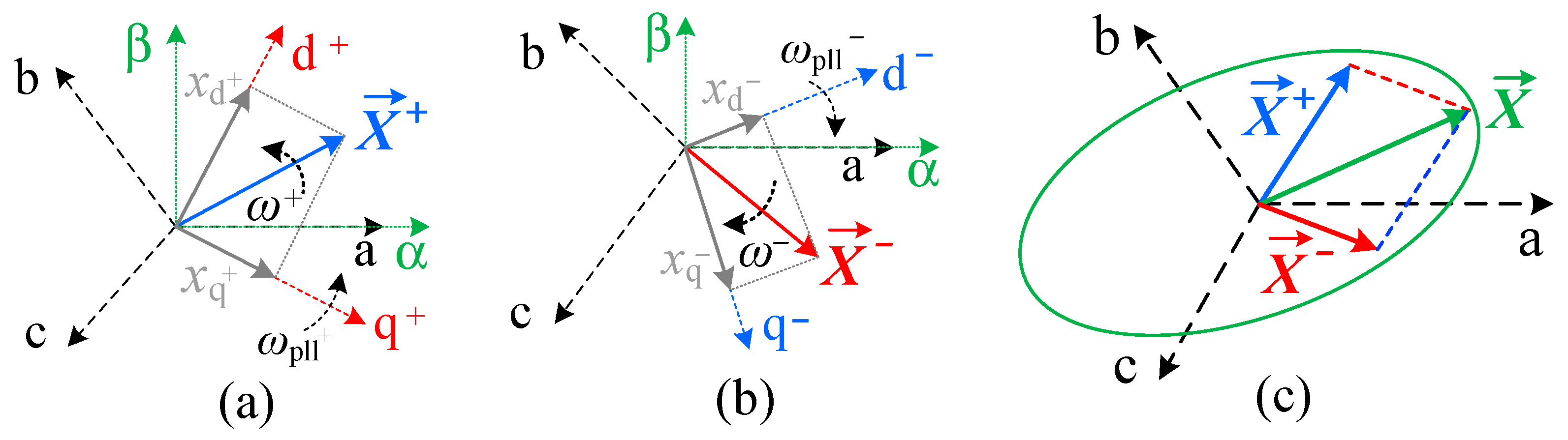
3.1. Coordinate System

The coordinate system used for modeling in this paper is shown in Figure 7, where abc is the three-phase stationary coordinate system, αβ is the two-phase stationary coordinate system, d⁺q⁺ is the two-phase positive-sequence (PS) rotating coordinate system, and d⁻q⁻ is the two-phase negative-sequence (NS) rotating coordinate system. For Figure 7a–c, the details are as follows:

As shown in Figure 7a, for the d⁺q⁺ coordinate system, the q⁺-axis lags the d⁺-axis by 90°, and the d⁺-axis is oriented in the direction of the positive-sequence voltage vector of PCC.

As shown in Figure 7b, for the d⁻q⁻ coordinate system, the q⁻-axis exceeds the d⁻-axis by 90°, and the d⁺-axis is oriented in the direction of the negative-sequence voltage vector of PCC.

As shown in Figure 7c, the synthetic vector of the PS and NS vectors is denoted as $\overrightarrow{\mathit{X}}$. The NS vector is usually non-zero under asymmetrical faults, and thus the trajectory of the endpoints of the synthetic vector is an ellipse when the synthetic vector is rotated by one week.

As shown in Figure 1, the high-voltage-side zero-sequence circuit is closed through the grounding connection of the neutral point. However, the low-voltage-side zero-sequence circuit is open. Thus, the voltages and currents of the VSC, denoted as x_abc, contain only PS and NS components. The vectors (complex vectors) of the symmetrical PS components and NS components can be denoted by ${\overrightarrow{\mathit{X}}}^{+}={\mathit{X}}^{+}{e}^{j({\omega }_{0}t+{\phi }^{+})}$ and ${\overrightarrow{\mathit{X}}}^{-}={\mathit{X}}^{-}{e}^{j(-{\omega }_{0}t+{\phi }^{-})}$, respectively, where X⁺ and X⁻ are the amplitude of the PS and NS components of x_abc, respectively, while φ⁺ and φ⁻ are the initial phase angle of the PS and NS components of x_abc, respectively.

The phasors of ${\overrightarrow{\mathit{X}}}^{+}$ and ${\overrightarrow{\mathit{X}}}^{-}$ are defined via the symmetrical components method as ${\dot{\mathit{X}}}^{+}={\mathit{X}}^{+}{e}^{j{\phi }^{+}}$ and ${\dot{\mathit{X}}}^{-}={\mathit{X}}^{-}{e}^{j{\phi }^{-}}$, respectively. The relationship between the vectors and the phasors is then expressed by Equation (1).

$${\overrightarrow{\mathit{X}}}^{+}={\dot{\mathit{X}}}^{+}{e}^{j{\omega }_{0}t},{\overrightarrow{\mathit{X}}}^{-}={\dot{\mathit{X}}}^{-}{e}^{-j{\omega }_{0}t}$$

(1)

The synthetic vector of the PS and NS vectors is denoted as $\overrightarrow{\mathit{X}}$, and the specific expression is shown in (2). The NS vector is usually non-zero under asymmetrical faults, and thus the trajectory of the endpoints of the synthetic vector is an ellipse when the synthetic vector is rotated by one week, as shown in Figure 7. The projection of the synthetic vector under the abc coordinate axis corresponds to the x_abc instantaneous value.

$$\overrightarrow{\mathit{X}}={\overrightarrow{\mathit{X}}}^{+}+{\overrightarrow{\mathit{X}}}^{-}$$

(2)

As can be seen from Figure 7, the transformation relations of the positive- and negative-sequence vectors ${\overrightarrow{\mathit{X}}}^{+}$ and ${\overrightarrow{\mathit{X}}}^{-}$ in the αβ and dq coordinate systems are shown in Equations (3) and (4), respectively.

$$\{\begin{array}{l}{\overrightarrow{\mathit{X}}}^{+}={{\overrightarrow{\mathit{X}}}_{\alpha }}^{+}+j{{\overrightarrow{\mathit{X}}}_{\beta }}^{+}\triangleq {{\overrightarrow{\mathit{X}}}_{\alpha \beta }}^{+}\\ {\overrightarrow{\mathit{X}}}^{-}={{\overrightarrow{\mathit{X}}}_{\alpha }}^{-}+j{{\overrightarrow{\mathit{X}}}_{\beta }}^{-}\triangleq {{\overrightarrow{\mathit{X}}}_{\alpha \beta }}^{-}\end{array}$$

(3)

$$\{\begin{array}{l}{\overrightarrow{\mathit{X}}}^{+}={({{\mathit{X}}_d}^{+}+j{{\mathit{X}}_q}^{+})}^{*}{e}^{j{{\theta }_{\mathrm{pll}}}^{+}}\triangleq {({{\mathit{X}}_{dq}}^{+})}^{*}{e}^{j{{\theta }_{\mathrm{pll}}}^{+}}\\ {\overrightarrow{\mathit{X}}}^{-}={({{\mathit{X}}_d}^{-}+j{{\mathit{X}}_q}^{-})}^{*}{e}^{j{{\theta }_{\mathrm{pll}}}^{-}}\triangleq {({{\mathit{X}}_{dq}}^{-})}^{*}{e}^{j{{\theta }_{\mathrm{pll}}}^{-}}\end{array}$$

(4)

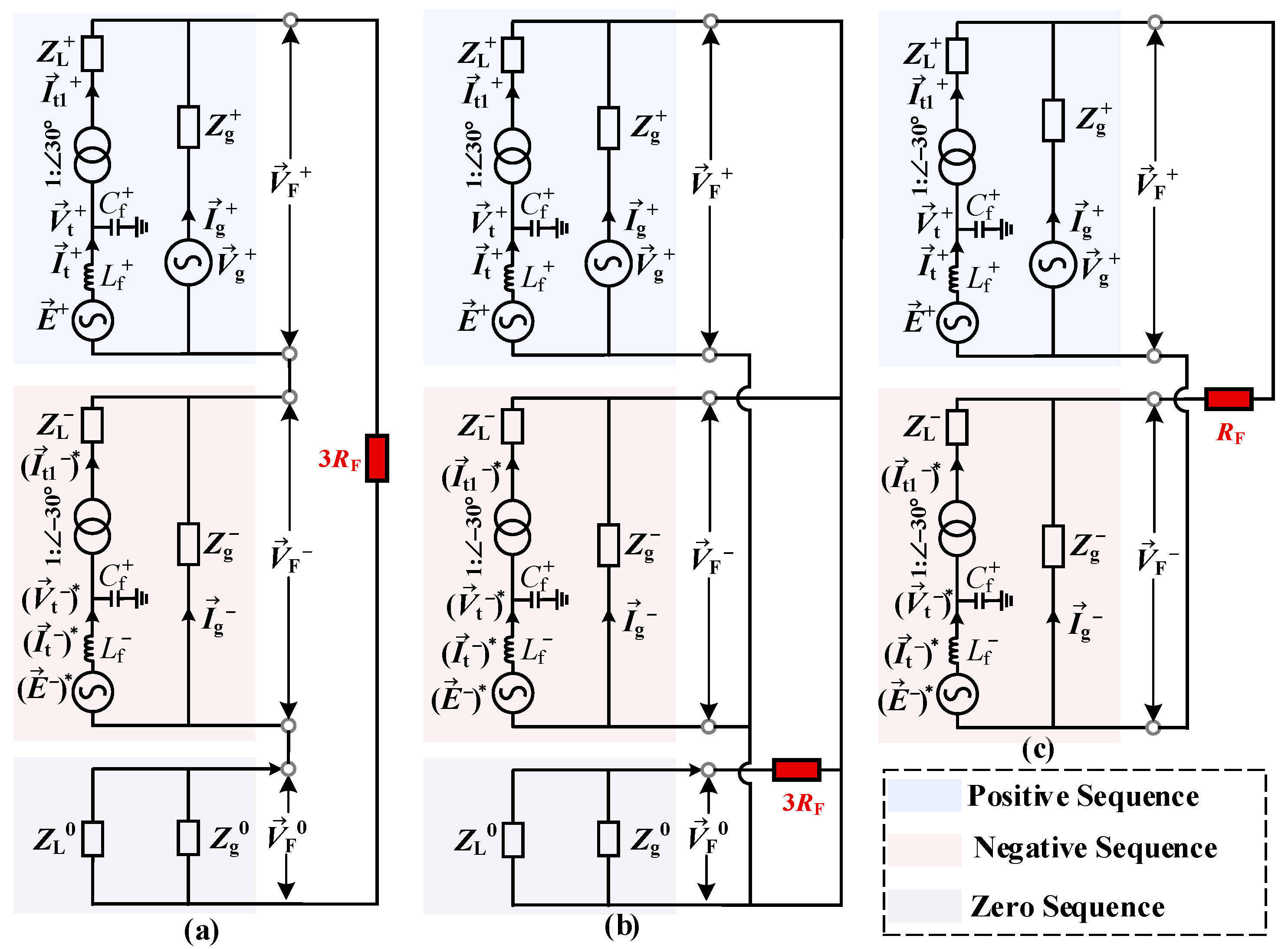
3.2. Main Circuit Modeling

Under different types of faults, the boundary conditions of the fault points are different. Based on the boundary conditions under different fault types, the interconnection of the sequence network under single line-to-ground (SLG), double line-to-ground (DLG), and line-to-line (LL) can be represented, as shown in Figure 8, where R_F represents the ground resistance. Note that Z_i⁺, Z_i⁻, and Z_i⁰ (i = L, g) represent positive, negative, and zero sequence impedances, respectively. For Figure 8a–c, the details are as follows:

Figure 8a presents the composite sequence network of the system under single line-to-ground faults.

Figure 8b presents the composite sequence network of the system under double line-to-ground faults.

Figure 8c presents the composite sequence network of the system under line-to-line faults.

Based on the circuit shown in Figure 8 and combined with the circuit graph theory, ${{\overrightarrow{\mathit{I}}}_t}^{+}$, ${{\overrightarrow{\mathit{I}}}_{t1}}^{+}$, ${{\overrightarrow{\mathit{I}}}_{t1}}^{-}$, ${{\overrightarrow{\mathit{I}}}_t}^{+}$, ${{\overrightarrow{\mathit{V}}}_t}^{+}$, ${{\overrightarrow{\mathit{V}}}_t}^{-}$ and ${{\overrightarrow{\mathit{I}}}_g}^{+}$ can be chosen as the state variables. Then, the state equation of the main circuit can be obtained based on Kirchhoff current law (KCL) and Kirchhoff voltage law (KVL), as shown in Equations (5) and (6).

$$\{\begin{array}{l}{\displaystyle \frac{d{{\overrightarrow{\mathit{I}}}_{t1}}^{+}}{dt}}=a_{11}{{\overrightarrow{\mathit{I}}}_{t1}}^{+}{e}^{j\pi /6}+a_{12}{{\overrightarrow{\mathit{I}}}_g}^{+}+a_{13}{({{\overrightarrow{\mathit{I}}}_{t1}}^{-})}^{*}{e}^{-j\pi /6}+a_{14}{{\overrightarrow{\mathit{V}}}_t}^{+}{e}^{j\pi /6}+a_{15}{{\overrightarrow{\mathit{V}}}_g}^{+}+a_{16}{({{\overrightarrow{\mathit{V}}}_t}^{-})}^{*}{e}^{-j\pi /6}\\ {\displaystyle \frac{d{{\overrightarrow{\mathit{I}}}_g}^{+}}{dt}}=a_{21}{{\overrightarrow{\mathit{I}}}_{t1}}^{+}{e}^{j\pi /6}+a_{22}{{\overrightarrow{\mathit{I}}}_g}^{+}+a_{23}{({{\overrightarrow{\mathit{I}}}_{t1}}^{-})}^{*}{e}^{-j\pi /6}+a_{24}{{\overrightarrow{\mathit{V}}}_t}^{+}{e}^{j\pi /6}+a_{25}{{\overrightarrow{\mathit{V}}}_g}^{+}+a_{26}{({{\overrightarrow{\mathit{V}}}_t}^{-})}^{*}{e}^{-j\pi /6}\\ {\displaystyle \frac{d{{\overrightarrow{\mathit{V}}}_t}^{+}}{dt}}=({{\overrightarrow{\mathit{I}}}_t}^{+}-{{\overrightarrow{\mathit{I}}}_{t1}}^{+})/{C_f}^{+}\\ {\displaystyle \frac{d{{\overrightarrow{\mathit{I}}}_t}^{+}}{dt}}=({\overrightarrow{\mathit{E}}}^{+}-{{\overrightarrow{\mathit{V}}}_t}^{+})/{L_f}^{+}\end{array}$$

(5)

$$\{\begin{array}{l}{\displaystyle \frac{d{({{\overrightarrow{\mathit{I}}}_{t1}}^{-})}^{*}}{dt}}=a_{31}{{\overrightarrow{\mathit{I}}}_{t1}}^{+}{e}^{j\pi /6}+a_{32}{{\overrightarrow{\mathit{I}}}_g}^{+}+a_{33}{({{\overrightarrow{\mathit{I}}}_{t1}}^{-})}^{*}{e}^{-j\pi /6}+a_{34}{{\overrightarrow{\mathit{V}}}_t}^{+}{e}^{j\pi /6}+a_{35}{{\overrightarrow{\mathit{V}}}_g}^{+}+a_{36}{({{\overrightarrow{\mathit{V}}}_t}^{-})}^{*}{e}^{-j\pi /6}\\ {\displaystyle \frac{d{({{\overrightarrow{\mathit{V}}}_t}^{-})}^{*}}{dt}}=\left({({{\overrightarrow{\mathit{I}}}_t}^{-})}^{*}-{({{\overrightarrow{\mathit{I}}}_{t1}}^{-})}^{*}\right)/{C_f}^{-}\\ {\displaystyle \frac{d{({{\overrightarrow{\mathit{I}}}_t}^{-})}^{*}}{dt}}=\left({({\overrightarrow{\mathit{E}}}^{-})}^{*}-{({{\overrightarrow{\mathit{V}}}_t}^{-})}^{*}\right)/{L_f}^{-}\end{array}$$

(6)

where a_ij (i = 1, 2, 3, j = 1, …, 6) is related to the type of fault. Taking the DLG fault as an example, the expressions for a_ij are provided in Appendix B.

Transforming Equations (5) and (6) into the rotating coordinate system d⁺q⁺ and d⁻q⁻, respectively, by using the coordinate transformation in (4), we obtain the following:

$$\{\begin{array}{l}{\displaystyle \frac{d{{\mathit{I}}_{t1dq}}^{+}}{dt}}=\left(\begin{array}{l}j{{\omega }_{\mathrm{pll}}}^{+}{{\mathit{I}}_{t1dq}}^{+}+a_{11}{{\mathit{I}}_{t1dq}}^{+}{e}^{-j\pi /6}+a_{12}{{\mathit{I}}_{gdq}}^{+}+a_{13}{({{\mathit{I}}_{t1dq}}^{-})}^{*}{e}^{j({{\theta }_{\mathrm{pll}}}^{-}+{{\theta }_{\mathrm{pll}}}^{+}+\pi /6)}+\\ a_{14}{{\mathit{V}}_{tdq}}^{+}{e}^{-j\pi /6}+a_{15}{{\mathit{V}}_g}^{+}{e}^{-j({{\theta }_g}^{+}-{{\theta }_{\mathrm{pll}}}^{+})}+a_{16}{({{\mathit{V}}_{tdq}}^{-})}^{*}{e}^{j({{\theta }_{\mathrm{pll}}}^{-}+{{\theta }_{\mathrm{pll}}}^{+}+\pi /6)}\end{array}\right)\\ {\displaystyle \frac{d{{\mathit{I}}_{gdq}}^{+}}{dt}}=\left(\begin{array}{l}j{{\omega }_{\mathrm{pll}}}^{+}{{\mathit{I}}_{gdq}}^{+}+a_{21}{{\mathit{I}}_{t1dq}}^{+}{e}^{-j\pi /6}+a_{22}{{\mathit{I}}_{gdq}}^{+}+a_{23}{({{\mathit{I}}_{t1dq}}^{-})}^{*}{e}^{j({{\theta }_{\mathrm{pll}}}^{-}+{{\theta }_{\mathrm{pll}}}^{+}+\pi /6)}+\\ a_{24}{{\mathit{V}}_{tdq}}^{+}{e}^{-j\pi /6}+a_{25}{{\mathit{V}}_g}^{+}{e}^{-j({{\theta }_g}^{+}-{{\theta }_{\mathrm{pll}}}^{+})}+a_{26}{({{\mathit{V}}_{tdq}}^{-})}^{*}{e}^{j({{\theta }_{\mathrm{pll}}}^{-}+{{\theta }_{\mathrm{pll}}}^{+}+\pi /6)}\end{array}\right)\\ {\displaystyle \frac{d{{\mathit{V}}_{tdq}}^{+}}{dt}}=j{{\omega }_{\mathrm{pll}}}^{+}{{\mathit{V}}_{tdq}}^{+}+({{\mathit{I}}_{tdq}}^{+}-{{\mathit{I}}_{t1dq}}^{+})/{C_f}^{+}\\ {\displaystyle \frac{d{{\mathit{I}}_{tdq}}^{+}}{dt}}=j{{\omega }_{\mathrm{pll}}}^{+}{{\mathit{I}}_{tdq}}^{+}+({{\mathit{E}}_{dq}}^{+}-{{\mathit{V}}_{tdq}}^{+})/{L_f}^{+}\end{array}$$

(7)

$$\{\begin{array}{l}{\displaystyle \frac{d{{\mathit{I}}_{t1dq}}^{-}}{dt}}=\left(\begin{array}{l}j{{\omega }_{\mathrm{pll}}}^{-}{{\mathit{I}}_{t1dq}}^{-}+a_{31}{\left({{\mathit{I}}_{t1dq}}^{+}\right)}^{*}{e}^{j({{\theta }_g}^{+}+{{\theta }_{\mathrm{pll}}}^{-}+j\pi /6)}+a_{32}{\left({{\mathit{I}}_{gdq}}^{+}\right)}^{*}{e}^{j({{\theta }_g}^{+}+{{\theta }_{\mathrm{pll}}}^{-})}+\\ a_{33}{{\mathit{I}}_{t1dq}}^{-}{e}^{-j\pi /6}+a_{34}{\left({{\mathit{V}}_{tdq}}^{+}\right)}^{*}{e}^{j({{\theta }_g}^{+}+{{\theta }_{\mathrm{pll}}}^{-}+j\pi /6)}+a_{35}{{\mathit{V}}_g}^{+}{e}^{j({{\theta }_g}^{+}+{{\theta }_{\mathrm{pll}}}^{-})}+a_{36}{{\mathit{V}}_{tdq}}^{-}{e}^{-j\pi /6}\end{array}\right)\\ {\displaystyle \frac{d{{\mathit{V}}_{tdq}}^{-}}{dt}}=j{{\omega }_{\mathrm{pll}}}^{-}{{\mathit{V}}_{tdq}}^{-}+\left({{\mathit{I}}_{tdq}}^{-}-{{\mathit{I}}_{t1dq}}^{-}\right)/{C_f}^{-}\\ {\displaystyle \frac{d{{\mathit{I}}_{tdq}}^{-}}{dt}}=j{{\omega }_{\mathrm{pll}}}^{-}{{\mathit{I}}_{tdq}}^{-}+\left({{\mathit{E}}_{dq}}^{-}-{{\mathit{V}}_{tdq}}^{-}\right)/{L_f}^{-}\end{array}$$

(8)

Equations (7) and (8) are the mathematical model of the main circuit, denoted as ${\dot{\mathit{X}}}_{\mathrm{Net}}$ = f(X_Net, Y_Net), where X_Net is the state variable vectors and Y_Net is the input variable vectors. The specific expressions for X_Net and Y_Net are given below:

$$\{\begin{array}{l}{\mathit{X}}_{\mathrm{Net}}={[{I_{t1d}}^{+},{I_{t1q}}^{+},{I_{gd}}^{+},{I_{gq}}^{+},{V_{td}}^{+},{V_{tq}}^{+},{I_{td}}^{+},{I_{tq}}^{+},{I_{t1d}}^{-},{I_{t1q}}^{-},{V_{td}}^{-},{V_{tq}}^{-},{I_{td}}^{-},{I_{tq}}^{-}]}^{\mathrm{T}}\\ {\mathit{Y}}_{\mathrm{Net}}={[{{\omega }_{\mathrm{pll}}}^{+},{{\omega }_{\mathrm{pll}}}^{-},{{\theta }_{\mathrm{pll}}}^{+},{{\theta }_{\mathrm{pll}}}^{-},{E_d}^{+},{E_q}^{+},{E_d}^{-},{E_q}^{-}]}^{\mathrm{T}}\end{array}$$

(9)

3.3. Control Modeling

From Figure 1, the control of the system includes DSOGI/PNSC, PLL⁺, PLL⁻, and a PR-based current controller, and this paper models the above controls in turn.

(a)

DSOGI/PNSC modeling

From Figure 1, the input of DSOGI is ${\overrightarrow{\mathit{V}}}_{t\alpha \beta }$ and the output is ${\widehat{\overrightarrow{\mathit{V}}}}_{t\alpha \beta }$ and its quadrature signal ${\widehat{\overrightarrow{\mathit{U}}}}_{t\alpha \beta }$. The control structure based on SOGI-QSG can be obtained as follows:

$$\{\begin{array}{l}d{\widehat{\overrightarrow{\mathit{V}}}}_{t\alpha }/dt={\omega }_0{k}_{\mathrm{SOGI}}\left({\overrightarrow{\mathit{V}}}_{t\alpha }-{\widehat{\overrightarrow{\mathit{V}}}}_{t\alpha }\right)-{\omega }_0{\widehat{\overrightarrow{\mathit{U}}}}_{t\alpha }\\ d{\widehat{\overrightarrow{\mathit{U}}}}_{t\alpha }/dt={\omega }_0{\widehat{\overrightarrow{\mathit{V}}}}_{t\alpha }\end{array}\hspace{1em}\hspace{1em}\{\begin{array}{l}d{\widehat{\overrightarrow{\mathit{V}}}}_{t\beta }/dt={\omega }_0{k}_{\mathrm{SOGI}}\left({\overrightarrow{\mathit{V}}}_{t\beta }-{\widehat{\overrightarrow{\mathit{V}}}}_{t\beta }\right)-{\omega }_0{\widehat{\overrightarrow{\mathit{U}}}}_{t\beta }\\ d{\widehat{\overrightarrow{\mathit{U}}}}_{t\beta }/dt={\omega }_0{\widehat{\overrightarrow{\mathit{V}}}}_{t\beta }\end{array}$$

(10)

where k_SOGI is the proportional gain coefficient of SOGI.

The mathematical model of DSOGI can be obtained by sorting out Equation (10) as shown in Equation (11).

$$\{\begin{array}{l}d{\widehat{\overrightarrow{\mathit{V}}}}_{t\alpha \beta }/dt={\omega }_0{k}_{\mathrm{SOGI}}\left({\overrightarrow{\mathit{V}}}_{t\alpha \beta }-{\widehat{\overrightarrow{\mathit{V}}}}_{t\alpha \beta }\right)-{\omega }_0{\widehat{\overrightarrow{\mathit{U}}}}_{t\alpha \beta }\\ d{\widehat{\overrightarrow{\mathit{U}}}}_{t\alpha \beta }/dt={\omega }_0{\widehat{\overrightarrow{\mathit{V}}}}_{t\alpha \beta }\end{array}$$

(11)

where k_SOGI is the proportional gain coefficient of SOGI.

Based on the control structure of the PNSC, the positive-sequence and negative-sequence components ${{\widehat{\overrightarrow{\mathit{V}}}}_{t\alpha \beta }}^{+}$ and ${{\widehat{\overrightarrow{\mathit{V}}}}_{t\alpha \beta }}^{-}$ of ${\widehat{\overrightarrow{\mathit{V}}}}_{t\alpha \beta }$ can be expressed, respectively, as follows:

$$\{\begin{array}{l}{{\widehat{\overrightarrow{\mathit{V}}}}_{t\alpha \beta }}^{+}={{\widehat{\overrightarrow{\mathit{V}}}}_{t\alpha }}^{+}+j{{\widehat{\overrightarrow{\mathit{V}}}}_{t\beta }}^{+}={\displaystyle \frac{1}{2}}\left({\widehat{\overrightarrow{\mathit{V}}}}_{t\alpha }+j{\widehat{\overrightarrow{\mathit{V}}}}_{t\beta }-{\widehat{\overrightarrow{\mathit{U}}}}_{t\beta }+j{\widehat{\overrightarrow{\mathit{U}}}}_{t\alpha }\right)={\displaystyle \frac{1}{2}}\left({\widehat{\overrightarrow{\mathit{V}}}}_{t\alpha \beta }+j{\widehat{\overrightarrow{\mathit{U}}}}_{t\alpha \beta }\right)\\ {{\widehat{\overrightarrow{\mathit{V}}}}_{t\alpha \beta }}^{-}={{\widehat{\overrightarrow{\mathit{V}}}}_{t\alpha }}^{-}+j{{\widehat{\overrightarrow{\mathit{V}}}}_{t\beta }}^{-}={\displaystyle \frac{1}{2}}\left({\widehat{\overrightarrow{\mathit{V}}}}_{t\alpha }+{\widehat{\overrightarrow{\mathit{U}}}}_{t\beta }+j{\widehat{\overrightarrow{\mathit{V}}}}_{t\beta }-j{\widehat{\overrightarrow{\mathit{U}}}}_{t\alpha }\right)={\displaystyle \frac{1}{2}}\left({\widehat{\overrightarrow{\mathit{V}}}}_{t\alpha \beta }-j{\widehat{\overrightarrow{\mathit{U}}}}_{t\alpha \beta }\right)\end{array}$$

(12)

Combining (12) and (13) and transforming it into the rotating coordinate system d⁺q⁺ and d⁻q⁻, the mathematical model of DSOGI/PNSC can be obtained as shown below:

$$\{\begin{array}{l}{\displaystyle \frac{d{{\widehat{\mathit{V}}}_{tdq}}^{+}}{dt}}=j{{\omega }_{\mathrm{pll}}}^{+}{{\widehat{\mathit{V}}}_{tdq}}^{+}+{\omega }_0{k}_{\mathrm{SOGI}}\left({{\mathit{V}}_{tdq}}^{+}-{{\widehat{\mathit{V}}}_{tdq}}^{+}\right)-{\omega }_0{{\widehat{\mathit{U}}}_{tdq}}^{+}\\ {\displaystyle \frac{d{{\widehat{\mathit{U}}}_{tdq}}^{+}}{dt}}=j{{\omega }_{\mathrm{pll}}}^{+}{{\widehat{\mathit{U}}}_{tdq}}^{+}+{\omega }_0{{\widehat{\mathit{V}}}_{tdq}}^{+}\end{array}$$

(13)

$$\{\begin{array}{l}{\displaystyle \frac{d{{\widehat{\mathit{V}}}_{tdq}}^{-}}{dt}}=j{{\omega }_{\mathrm{pll}}}^{-}{{\widehat{\mathit{V}}}_{tdq}}^{-}+{\omega }_0{k}_{\mathrm{SOGI}}\left({{\mathit{V}}_{tdq}}^{-}-{{\widehat{\mathit{V}}}_{tdq}}^{-}\right)-{\omega }_0{{\widehat{\mathit{U}}}_{tdq}}^{-}\\ {\displaystyle \frac{d{{\widehat{\mathit{U}}}_{tdq}}^{-}}{dt}}=j{{\omega }_{\mathrm{pll}}}^{-}{{\widehat{\mathit{U}}}_{tdq}}^{-}+{\omega }_0{{\widehat{\mathit{V}}}_{tdq}}^{-}\end{array}$$

(14)

Equations (13) and (14) are the mathematical model of the DSOGI/PNSC, denoted as ${\dot{\mathit{X}}}_{\mathrm{D}/\mathrm{P}}$ = f_D/P(X_D/P, Y_D/P), where X_D/P is the state variable vectors and Y_D/P is the input variable vectors. The specific expressions for X_D/P and Y_D/P are given below:

$$\{\begin{array}{l}{\mathit{X}}_{\mathrm{D}/\mathrm{P}}={[{{\widehat{V}}_{td}}^{+},{{\widehat{V}}_{tq}}^{+},{{\widehat{\mathit{U}}}_{td}}^{+},{{\widehat{\mathit{U}}}_{tq}}^{+},{{\widehat{V}}_{td}}^{-},{{\widehat{V}}_{tq}}^{-},{{\widehat{\mathit{U}}}_{td}}^{-},{{\widehat{\mathit{U}}}_{tq}}^{-}]}^T\\ {\mathit{Y}}_{\mathrm{D}/\mathrm{P}}={[{V_{td}}^{+},{V_{tq}}^{+},{V_{td}}^{-},{V_{tq}}^{-}]}^T\end{array}$$

(15)

(b)

PLL⁺ and PLL⁻ modeling

The output phase angles θ_pll⁺ and θ_pll⁻ of PLL⁺ and PLL⁻ can be expressed as Equations (16) and (17), respectively.

$$\{\begin{array}{l}{\displaystyle \frac{d{{\theta }_{\mathrm{pll}}}^{+}}{dt}}=-k_p{{\widehat{V}}_{tq}}^{+}-k_i{x_{\mathrm{pll}}}^{+}+{\omega }_0\triangleq {{\omega }_{\mathrm{pll}}}^{+}\\ {\displaystyle \frac{d{x_{\mathrm{pll}}}^{+}}{dt}}={{\widehat{V}}_{tq}}^{+}\end{array}$$

(16)

$$\{\begin{array}{l}{\displaystyle \frac{d{{\theta }_{\mathrm{pll}}}^{-}}{dt}}=-k_p{{\widehat{V}}_{tq}}^{-}-k_i{x_{\mathrm{pll}}}^{-}-{\omega }_0\triangleq {{\omega }_{\mathrm{pll}}}^{-}\\ {\displaystyle \frac{d{x_{\mathrm{pll}}}^{-}}{dt}}={{\widehat{V}}_{tq}}^{-}\end{array}$$

(17)

where k_p and k_i are the proportional and integral coefficients of the PLL, respectively.

Equations (16) and (17) are the mathematical model of the PLL, denoted as ${\dot{\mathit{X}}}_{PLL}$ = f_PLL(X_PLL, Y_PLL), where X_PLL is the state variable vectors and Y_PLL is the input variable vectors. The specific expressions for X_PLL and Y_PLL are given below:

$${\mathit{X}}_{\mathrm{PLL}}={[{{\theta }_{\mathrm{pll}}}^{+},{{\theta }_{\mathrm{pll}}}^{-},{x_{\mathrm{pll}}}^{+},{x_{\mathrm{pll}}}^{-}]}^{\mathrm{T}};{\mathit{Y}}_{\mathrm{PLL}}={[{{\widehat{\mathit{V}}}_{\mathrm{t}q}}^{+},{{\widehat{\mathit{V}}}_{\mathrm{t}q}}^{-}]}^{\mathrm{T}}$$

(18)

(c)

PR-based current controller modeling

As can be seen from the control structure of the PR-based current controller, the output voltage of the VSC $\overrightarrow{\mathit{E}}$ can be expressed in Equation (19).

$$\left({{\overrightarrow{\mathit{E}}}_{\alpha \beta }}^{+}+{{\overrightarrow{\mathit{E}}}_{\alpha \beta }}^{-}\right)=\left(k_{p\_pr}+{\displaystyle \frac{2k_{r\_pr}{\omega }_{c}s}{s^2+2{\omega }_{c}s+{\omega }_0^2}}\right)\left\{\left({\overrightarrow{\mathit{I}}}_{tref\alpha \beta }^{+}+{\overrightarrow{\mathit{I}}}_{tref\alpha \beta }^{-}\right)-\left({{\overrightarrow{\mathit{I}}}_{t\alpha \beta }}^{+}+{{\overrightarrow{\mathit{I}}}_{t\alpha \beta }}^{-}\right)\right\}+\left({{\overrightarrow{\mathit{V}}}_{t\alpha \beta }}^{+}+{{\overrightarrow{\mathit{V}}}_{t\alpha \beta }}^{-}\right)$$

(19)

where $k_{p\_pr}$, $k_{r\_pr}$ and ω_c are the proportional gain, resonance gain, and resonance bandwidth coefficient of the PR-based current controller, respectively. The expressions of ${\overrightarrow{\mathit{I}}}_{tref\alpha \beta }^{+}$ and ${\overrightarrow{\mathit{I}}}_{tref\alpha \beta }^{-}$ are shown in the following.

$${\overrightarrow{\mathit{I}}}_{tref\alpha \beta }^{+}={\overrightarrow{\mathit{I}}}_{trefdq}^{+}{e}^{j{{\theta }_{\mathrm{pll}}}^{+}};{\overrightarrow{\mathit{I}}}_{tref\alpha \beta }^{-}={\overrightarrow{\mathit{I}}}_{trefdq}^{-}{e}^{j{{\theta }_{\mathrm{pll}}}^{-}}$$

(20)

Both sides of (19) are multiplied by $(s^2+2{\omega }_{c}s+{\omega }_0^2)/s^2$ and transformed into the rotating coordinate system d⁺q⁺ and d⁻q⁻, respectively, which leads to (21) and (22):

$$\{\begin{array}{l}{\displaystyle \frac{d{{\mathit{x}}_{pr1dq}}^{+}}{dt}}=j{{\omega }_{\mathrm{pll}}}^{+}{{\mathit{x}}_{pr1dq}}^{+}+{{\mathit{I}}_{trefdq}}^{+}-{{\mathit{I}}_{tdq}}^{+}\\ {\displaystyle \frac{d{{\mathit{x}}_{pr2dq}}^{+}}{dt}}=j{{\omega }_{\mathrm{pll}}}^{+}{{\mathit{x}}_{pr2dq}}^{+}+{{\mathit{x}}_{pr1dq}}^{+}\\ {\displaystyle \frac{d{{\mathit{x}}_{pr3dq}}^{+}}{dt}}=\left[\begin{array}{l}j{{\omega }_{\mathrm{pll}}}^{+}{{\mathit{x}}_{pr2dq}}^{+}+k_{p\_pr}\left({{\mathit{I}}_{trefdq}}^{+}-{{\mathit{I}}_{tdq}}^{+}\right)+\left(2k_{r\_pr}{\omega }_c+2{\omega }_c{k}_{p\_pr}\right){{\mathit{x}}_{pr1dq}}^{+}\\ +{\omega }_0^2{k}_{p\_pr}{{\mathit{x}}_{pr2dq}}^{+}-2{\omega }_c{{\mathit{x}}_{pr3dq}}^{+}-{\omega }_0^2{{\mathit{x}}_{pr4dq}}^{+}\end{array}\right]\\ {\displaystyle \frac{d{{\mathit{x}}_{pr4dq}}^{+}}{dt}}=j{{\omega }_{\mathrm{pll}}}^{+}{{\mathit{x}}_{pr4dq}}^{+}+{{\mathit{x}}_{pr3dq}}^{+}\end{array}$$

(21)

$$\{\begin{array}{l}{\displaystyle \frac{d{{\mathit{x}}_{pr1dq}}^{-}}{dt}}=j{{\omega }_{\mathrm{pll}}}^{-}{{\mathit{x}}_{pr1dq}}^{-}+{{\mathit{I}}_{trefdq}}^{-}-{{\mathit{I}}_{tdq}}^{-}\\ {\displaystyle \frac{d{{\mathit{x}}_{pr2dq}}^{-}}{dt}}=j{{\omega }_{\mathrm{pll}}}^{-}{{\mathit{x}}_{pr2dq}}^{-}+{{\mathit{x}}_{pr1dq}}^{-}\\ {\displaystyle \frac{d{{\mathit{x}}_{pr3dq}}^{-}}{dt}}=\left[\begin{array}{l}j{{\omega }_{\mathrm{pll}}}^{-}{{\mathit{x}}_{pr2dq}}^{-}+k_{p\_pr}\left({{\mathit{I}}_{trefdq}}^{-}-{{\mathit{I}}_{tdq}}^{-}\right)+\left(2k_{r\_pr}{\omega }_c+2{\omega }_c{k}_{p\_pr}\right){{\mathit{x}}_{pr1dq}}^{-}\\ +{\omega }_0^2{k}_{p\_pr}{{\mathit{x}}_{pr2dq}}^{-}-2{\omega }_c{{\mathit{x}}_{pr3dq}}^{-}-{\omega }_0^2{{\mathit{x}}_{pr4dq}}^{-}\end{array}\right]\\ {\displaystyle \frac{d{{\mathit{x}}_{pr4dq}}^{-}}{dt}}=j{{\omega }_{\mathrm{pll}}}^{-}{{\mathit{x}}_{pr4dq}}^{-}+{{\mathit{x}}_{pr3dq}}^{-}\end{array}$$

(22)

where

$$\{\begin{array}{l}{{\mathit{x}}_{pr1dq}}^{+}=e^{j{{\theta }_{\mathrm{pll}}}^{+}}{\displaystyle \int ({{\mathit{I}}_{trefdq}}^{+}-{{\mathit{I}}_{tdq}}^{+})e^{-j{{\theta }_{\mathrm{pll}}}^{+}}dt};{{\mathit{x}}_{pr2dq}}^{+}=e^{j{{\theta }_{\mathrm{pll}}}^{+}}{\displaystyle \int {{\mathit{x}}_{pr1dq}}^{+}{e}^{-j{{\theta }_{\mathrm{pll}}}^{+}}dt}\\ {{\mathit{x}}_{pr3dq}}^{+}=e^{j{{\theta }_{\mathrm{pll}}}^{+}}{\displaystyle \int ({{\mathit{E}}_{dq}}^{+}-{{\mathit{V}}_{tdq}}^{+})e^{-j{{\theta }_{\mathrm{pll}}}^{+}}dt;}{{\mathit{x}}_{pr4dq}}^{+}=e^{j{{\theta }_{\mathrm{pll}}}^{+}}{\displaystyle \int {{\mathit{x}}_{pr3dq}}^{+}{e}^{-j{{\theta }_{\mathrm{pll}}}^{+}}dt}\\ {{\mathit{x}}_{pr1dq}}^{-}=e^{j{{\theta }_{\mathrm{pll}}}^{-}}{\displaystyle \int ({{\mathit{I}}_{trefdq}}^{-}-{{\mathit{I}}_{tdq}}^{-})e^{-j{{\theta }_{\mathrm{pll}}}^{-}}dt};{{\mathit{x}}_{pr2dq}}^{+}=e^{j{{\theta }_{\mathrm{pll}}}^{+}}{\displaystyle \int {{\mathit{x}}_{pr1dq}}^{-}{e}^{-j{{\theta }_{\mathrm{pll}}}^{-}}dt}\\ {{\mathit{x}}_{pr3dq}}^{-}=e^{j{{\theta }_{\mathrm{pll}}}^{-}}{\displaystyle \int ({{\mathit{E}}_{dq}}^{-}-{{\mathit{V}}_{tdq}}^{-})e^{-j{{\theta }_{\mathrm{pll}}}^{-}}dt;}{{\mathit{x}}_{pr4dq}}^{-}=e^{j{{\theta }_{\mathrm{pll}}}^{-}}{\displaystyle \int {{\mathit{x}}_{pr3dq}}^{-}{e}^{-j{{\theta }_{\mathrm{pll}}}^{-}}dt}\end{array}$$

(23)

Equations (21) and (22) are the mathematical model of the PR-based current controller, denoted as ${\dot{\mathit{X}}}_{PR}$ = f_PR(X_PR, Y_PR), where X_PR is the state variable vectors and Y_PR is the input variable vectors. The specific expressions for X_PR and Y_PR are given below:

$$\{\begin{array}{l}{\mathit{X}}_{\mathrm{PR}}={\left[\begin{array}{l}{x_{pr1d}}^{+},{x_{pr1q}}^{+},{x_{pr2d}}^{+},{x_{pr2q}}^{+},{x_{pr3d}}^{+},{x_{pr3q}}^{+},{x_{pr4d}}^{+},{x_{pr4q}}^{+},\\ {x_{pr1d}}^{-},{x_{pr1q}}^{-},{x_{pr2d}}^{-},{x_{pr2q}}^{-},{x_{pr3d}}^{-},{x_{pr3q}}^{-},{x_{pr4d}}^{-},{x_{pr4q}}^{-}\end{array}\right]}^T\\ {\mathit{Y}}_{\mathrm{PR}}={[{{\omega }_{\mathrm{pll}}}^{+},{{\omega }_{\mathrm{pll}}}^{-},{I_{td}}^{+},{I_{tq}}^{+},{I_{td}}^{-},{I_{tq}}^{-},{I_{trefd}}^{+},{I_{trefq}}^{+},{I_{trefd}}^{-},{I_{trefq}}^{-}]}^T\end{array}$$

(24)

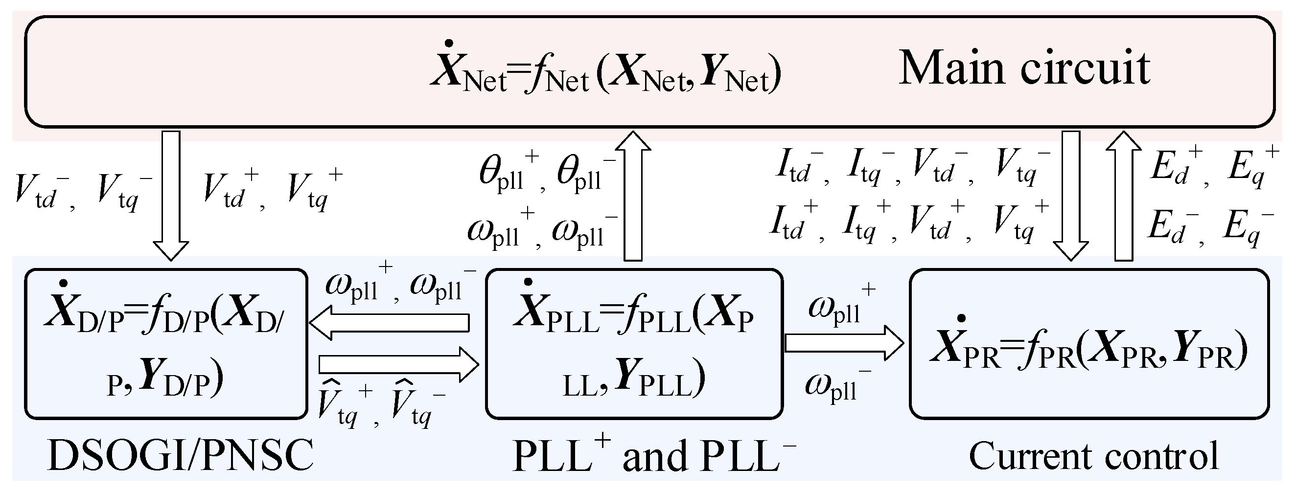
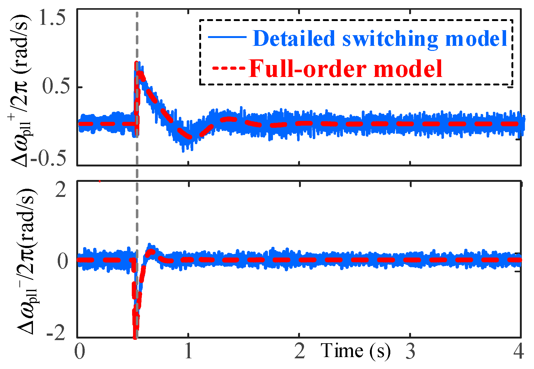
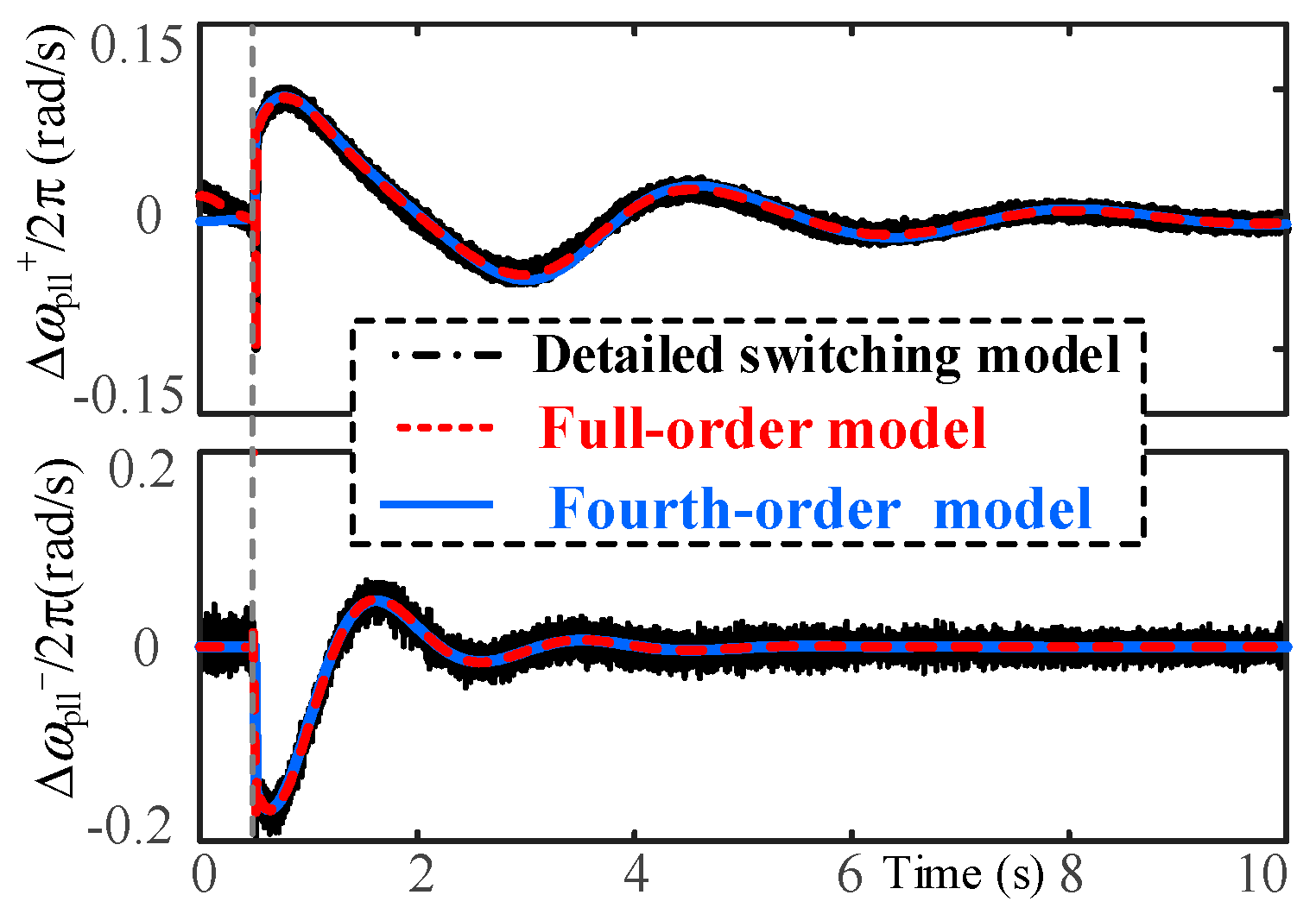
3.4. Complete Nonlinear Mathematical Model of the System and Validation

Combining the above mathematical model of the main circuit and control, the mathematical model of the system under asymmetric faults can be obtained, referred to as the full-order model in this paper, as shown in Figure 9.

To validate the accuracy of the full-order mathematical model, a detailed electromagnetic transient switching model of the grid-connected VSC system, as shown in Figure 1, was constructed in PSCAD/EMTDC. The system parameters are listed in Appendix A, Table A1. Figure 10 compares the simulation results of the full-order mathematical model with those of the detailed switching model for Case 1.

As can be seen from Figure 10, the transient waveforms of the full-order mathematical model and the detailed switching model are almost identical. This indicates that the full-order model constructed in this paper accurately reflects the transient behavior of the system during asymmetric faults and can be used for subsequent transient stability analysis.

4. Transient Stability Analysis

The full-order model of the grid-connected VSC system under asymmetrical faults is a nonlinear differential equation that cannot be solved analytically. Additionally, the full-order model is a high-order model with 42 state variables, which makes it almost impractical to use common methods such as Lyapunov’s direct method [12], linear matrix inequality (LMI) optimization method [13], or the sum-of-squares (SOS) programming method [12] to construct the largest estimated domain of attraction of the system for evaluating transient stability.

Thus, in this section, the phase trajectory method is used to analyze transient stability which can provide a simple and intuitive result of PLL-Syn transient stability. First, the phase trajectory method is briefly introduced in Section 4.1. Then, in Section 4.2, the transient stability of the system is analyzed based on the phase trajectory method. Finally, the conditions under which dynamics such as LC filter and AC network transient, current control dynamics, and the DSOGI//PNSC can be ignored are discussed in Section 4.3.

4.1. The Phase Trajectory Method

The steps for analyzing the transient stability of a system based on the phase trajectory method are briefly described as follows:

• Step 1: Determine Initial Conditions:

To analyze the transient stability of the system, start by specifying the initial conditions of the state variables in the phase space. Under normal operating conditions, the system predominantly exhibits positive sequence components. Consequently, the initial states of state variables associated with negative sequence dynamics are set to zero.

• Step 2: Solve Differential Equations:

Employ numerical simulation techniques, such as the Runge–Kutta method, to solve the system’s differential equations. This involves iteratively updating the values of the state variables to trace the system’s trajectory through phase space. The solution of these equations provides a dynamic representation of the system’s evolution over time.

• Step 3: Visualize Phase Trajectory:

Represent the system’s trajectory in phase space using phase diagrams or phase plane plots. Each point on the diagram corresponds to the system’s state at a particular moment, while the trajectory illustrates the system’s temporal evolution. Visualization helps in understanding how the state variables interact and evolve.

This method offers significant insights into system behavior and stability by analyzing how the system’s state evolves along its trajectory. The transient stability is assessed based on whether the trajectory converges or diverges. Notably, the phase trajectory method provides reliable stability assessment results without being overly conservative.

4.2. Transient Stability Analysis with the Phase Trajectory Method

Figure 11 shows the phase trajectories of the full-order model in the δ⁺-x_pll⁺-δ⁻ phase plane for Case 1.

As seen in Figure 11, the phase trajectory of the full-order model converges, indicating the transient synchronization stability of the system. This is consistent with the electromagnetic transient simulation results shown in Figure 10. Additionally, Figure 11 also presents the phase trajectories of the fourth-order model. The phase trajectory of the fourth-order model diverges, indicating the transient synchronization instability of the system. Therefore, the theoretical analysis results shown in Figure 11 demonstrate that the dynamic interaction between PR-based current control, DSOGI//PNSC, and PLL control enhances the transient stability of the system.

It is important to note that the analyses in [14,15,16] indicate that, under symmetrical fault conditions, the interaction between current control and PLL control can deteriorate the system’s transient stability. However, the theoretical analysis shown in Figure 11 suggests that, under asymmetrical fault conditions, the interaction of multiple control loops enhances the system’s transient stability.

4.3. Analysis of Condition for Considering Only PLL Dynamics

Based on the full-order model in this paper and the fourth-order models in [25], the system’s transient response can be obtained. We introduce the positive- and negative-sequence angular frequency peak error coefficients, denoted as e⁺ and e⁻, respectively, to quantitatively describe the deviation between the two models. The expressions for e⁺ and e⁻ are given in Equations (25) and (26). The schematic diagram of e⁺ is illustrated in Figure 12.

$$e^{+}=\left|\left(\Delta {{\omega }_{cmax}}^{+}-\Delta {{\omega }_{ncmax}}^{+}\right)/\Delta {{\omega }_{cmax}}^{+}\right|$$

(25)

$$e^{-}=\left|\left(\Delta {{\omega }_{cmax}}^{-}-\Delta {{\omega }_{ncmax}}^{-}\right)/\Delta {{\omega }_{cmax}}^{-}\right|$$

(26)

When both e⁺ and e⁻ are not greater than ε, it can be considered that the dynamic responses of the fourth-order model and the full-order model are consistent. Therefore, the fourth-order model, which only considers PLL dynamics, can be used to analyze the transient synchronization stability of the system under asymmetric faults. Here, ε represents an acceptable model error, typically less than 5%. Thus, the conditions under which the impacts of DSOGI//PNSC and PR-based current control dynamics can be ignored are e⁺ ≤ ε and e⁻ ≤ ε.

Through the above analysis, this paper delineates the PLL bandwidth threshold f_c, as shown in Figure 13. Mathematically, f_c can be described by (27). When the PLL bandwidth is less than f_c, the impacts of DSOGI//PNSC and PR-based current control dynamics can be ignored when analyzing the transient synchronization stability of the grid-connected VSC system.

$$max\{e^{+}(f_c),e^{-}(f_c)\}=\epsilon$$

(27)

Considering a DLG fault applied on phases b and c, the current references are selected as I_tdref⁺ = 0.4 pu, I_tqref⁺ = 0.5 pu, I_tdref⁻ = 0 pu, and I_tqref⁻ = 0.4 pu. Then, by enumerating, the detailed values of f_c in Figure 13 can be calculated to be 15 rad/s. To validate the effectiveness of the PLL bandwidth threshold delineated in this paper, the PLL bandwidth was reduced to 14.5 rad/s (k_p = 10, k_i = 50). This case is referred to as Case 2. Figure 14 compares the phase trajectories of the full-order and fourth-order models. As shown in Figure 14, the trajectories of the full-order and fourth-order nonlinear models in the δ⁺-x_pll⁺-δ⁻ plane are highly consistent. Additionally, Figure 15 compares the transient responses of the fourth-order, the full-order, and the detailed electromagnetic transient switching models. The figure shows that the responses of these three models are almost identical.

The results of Figure 14 and Figure 15 indicate that, when the PLL bandwidth is within the threshold defined by Equation (27), the impacts of DSOGI//PNSC and current control dynamics can be ignored. Consequently, the simplified fourth-order model can be used to analyze the transient synchronization stability of the system under asymmetric faults.

5. Conclusions

This paper analyzes the transient synchronization stability of grid-connected converters under asymmetric faults, with a focus on the coupling of multiple control loops. Our analysis shows that a fourth-order model, which only considers PLL dynamics, is insufficient to accurately represent the system’s dynamic characteristics when the PLL bandwidth is large and approaches the bandwidths of positive and negative sequence separation and current control. In contrast, the transient model we constructed, which accounts for the coupling of multiple control loops, accurately represents the system’s transient synchronization process, providing correct transient synchronization stability analysis results. Therefore, under conditions of high PLL bandwidth, only the full-order model can be used to reliably analyze the system’s transient synchronization stability.

Using this accurate full-order model, we applied the phase trajectory method to analyze the system’s transient synchronization stability and identified the PLL bandwidth boundary within which the effects of positive and negative sequence separation and current control dynamics can be ignored. When the PLL bandwidth is within this threshold, the fourth-order model, considering only PLL dynamics, can be effectively used to analyze the system’s transient synchronization stability under asymmetric faults. This conclusion also provides useful guidance for the design of PLL control parameters.

References

1. Zhou, Q.; Shahidehpour, M.; Alabdulwahab, A.; Abusorrah, A.M. Flexible Division and Unification Control Strategies for Resilience Enhancement in Networked Microgrids. IEEE Trans. Power Syst. 2020, 35, 474–486. [Google Scholar] [CrossRef]
2. Li, Y.; Gu, Y.; Green, T.C. Revisiting grid-forming and grid-following inverters: A duality theory. IEEE Trans. Power Syst. 2022, 37, 4541–4554. [Google Scholar] [CrossRef]
3. Taul, M.G.; Wang, X.; Davari, P.; Blaabjerg, F. An Overview of Assessment Methods for Synchronization Stability of Grid-Connected Converters under Severe Symmetrical Grid Faults. IEEE Trans. Power Electron. 2019, 34, 9655–9670. [Google Scholar] [CrossRef]
4. Sun, R.; Ma, J.; Yang, W.; Wang, S.; Liu, T. Transient synchronization stability control for LVRT with power angle estimation. IEEE Trans. Power Electron. 2021, 36, 10981–10985. [Google Scholar] [CrossRef]
5. Li, X.; Tian, Z.; Zha, X.; Sun, P.; Hu, Y.; Huang, M. An Iterative Equal Area Criterion for Transient Stability Analysis of Grid-tied Converter Systems with Varying Damping. IEEE Trans. Power Syst. 2023, 39, 1771–1784. [Google Scholar] [CrossRef]
6. He, X.; Geng, H.; Xi, J.; Guerrero, J.M. Resynchronization Analysis and Improvement of grid-connected VSCs during grid faults. IEEE J. Emerg. Sel. Top. Power Electron. 2021, 9, 438–445. [Google Scholar] [CrossRef]
7. Wu, H.; Wang, X. Design-Oriented Transient Stability Analysis of PLL-Synchronized Voltage-Source Converters. IEEE Trans. Power Electron. 2020, 35, 3573–3589. [Google Scholar] [CrossRef]
8. Wang, X.; Wu, H.; Wang, X.; Dall, L.; Kwon, J.B. Transient Stability Analysis of Grid-Following VSCs Considering Voltage-Dependent Current Injection during Fault Ride-Through. IEEE Trans. Energy Convers. 2022, 37, 2749–2760. [Google Scholar] [CrossRef]
9. Hu, Q.; Fu, L.; Ma, F.; Ji, F. Large Signal Synchronizing Instability of PLL-Based VSC Connected to Weak AC Grid. IEEE Trans. Power Syst. 2019, 34, 3220–3229. [Google Scholar] [CrossRef]
10. Hu, Q.; Fu, L.; Ma, F.; Wang, G.; Liu, C.; Ma, Y. Impact of LVRT Control on Transient Synchronizing Stability of PLL-Based Wind Turbine Converter Connected to High Impedance AC Grid. IEEE Trans. Power Syst. 2022, 38, 5445–5458. [Google Scholar] [CrossRef]
11. Zhang, Y.; Zhang, C.; Cai, X. Large-Signal Grid-synchronization Stability Analysis of PLL-based VSCs Using Lyapunov’s Direct Method. IEEE Trans. Power Syst. 2022, 37, 788–791. [Google Scholar] [CrossRef]
12. Zhang, Z.; Schuerhuber, R.; Fickert, L.; Friedl, K.; Chen, G.; Zhang, Y. Region of Attraction’s Estimation for Grid Connected Converters with Phase-Locked Loop. IEEE Trans. Power Syst. 2022, 37, 1351–1362. [Google Scholar] [CrossRef]
13. Li, X.; Wang, Z.; Liu, Y.; Wang, Z.; Zhu, L.; Guo, L.; Zhang, C.; Zhu, J.; Wang, C. The Largest Estimated Domain of Attraction and its Applications for Transient Stability Analysis of PLL Synchronization in Weak-Grid-Connected VSCs. IEEE Trans. Power Syst. 2023, 38, 4107–4121. [Google Scholar] [CrossRef]
14. Hu, Q.; Fu, L.; Ma, F.; Ji, F.; Zhang, Y. Analogized Synchronous-Generator Model of PLL-Based VSC and Transient Synchronizing Stability of Converter Dominated Power System. IEEE Trans. Sustain. Energy 2021, 12, 1174–1185. [Google Scholar] [CrossRef]
15. Liu, C.C.; Yang, J.; Tse, C.K.; Huang, M. Transient Synchronization Stability of Grid-Following Converters Considering Nonideal Current Loop. IEEE Trans. Power Electron. 2023, 38, 13757–13769. [Google Scholar] [CrossRef]
16. Wu, C.; Lyu, Y.; Wang, Y.; Blaabjerg, F. Transient Synchronization Stability Analysis of Grid-Following Converter Considering the Coupling Effect of Current Loop and Phase Locked Loop. IEEE Trans. Energy Convers. 2024, 39, 544–554. [Google Scholar] [CrossRef]
17. NERC. 1200 MW Fault Induced Solar Photovoltaic Resource Interruption Disturbance Report—Southern California 8/16/2016 Event. June 2017. Available online: www.nerc.com (accessed on 8 June 2017).
18. Göksu, Ö.; Teodorescu, R.; Bak, C.L.; Iov, F.; Kjær, P.C. Impact of wind power plant reactive current injection during asymmetrical grid faults. IET Renew. Power Gener. 2013, 7, 484–492. [Google Scholar] [CrossRef]
19. Taul, M.G.; Golestan, S.; Wang, X.; Davari, P.; Blaabjerg, F. Modeling of converter synchronization stability under grid faults: The general case. IEEE J. Emerg. Sel. Top. Power Electron. 2020, 10, 2790–2804. [Google Scholar] [CrossRef]
20. He, X.; He, C.; Pan, S.; Geng, H.; Liu, F. Synchronization Instability of Inverter-Based Generation during Asymmetrical Grid Faults. IEEE Trans. Power Syst. 2022, 37, 1018–1031. [Google Scholar] [CrossRef]
21. Liu, R.; Yao, J.; Sun, P.; Pei, J.; Zhang, H.; Zhao, Y. Complex Impedance-Based Frequency Coupling Characteristics Analysis of DFIG-Based WT during Asymmetric Grid Faults. IEEE Trans. Ind. Electron. 2021, 68, 8274–8288. [Google Scholar] [CrossRef]
22. Akhavan, A.; Golestan, S.; Vasquez, J.C.; Guerrero, J.M. Control and Stability Analysis of Current-Controlled Grid-Connected Inverters in Asymmetrical Grids. IEEE Trans. Power Electron. 2022, 37, 14252–14264. [Google Scholar] [CrossRef]
23. Li, Y.; Lin, C.; Hu, J.; Guo, J. PLL Synchronization Stability of Grid-Connected VSCs Under Asymmetric AC Faults. IEEE Trans. Energy Convers. 2022, 37, 2438–2448. [Google Scholar] [CrossRef]
24. Li, X.; Wang, Z.; Zhu, L.; Guo, L.; Wang, C. Analytical Dual-Sequence Current Injections Feasible Region of Weak-Grid Connected VSC under Asymmetric Grid Faults. IEEE Trans. Power Syst. 2023, 38, 5546–5559. [Google Scholar] [CrossRef]
25. Wang, Z.; Guo, L.; Li, X.; Pang, X.; Li, X.; Zhou, X.; Wang, C. PLL Synchronization Transient Stability Analysis of a Weak-Grid Connected VSC during Asymmetric Faults. IEEE Trans. Power Electron. 2024, 39, 2140–2154. [Google Scholar] [CrossRef]
Figure 1. Topology and control of the WG–VSC system during asymmetric faults.
Applsci 14 07834 g001
Figure 2. The control structure of DSOGI/PNSC: (a) DSOGI/PNSC; (b) SOGI-QSG; (c) PNSC.
Applsci 14 07834 g002
Figure 3. The control structure of PLL+ and PLL: (a) PLL+; (b) PLL.
Applsci 14 07834 g003
Figure 4. The control structure of PR-based dual-sequence current control.
Applsci 14 07834 g004
Figure 5. The equivalent circuit of the fourth-order model.
Applsci 14 07834 g005
Figure 6. Simulation results of the fourth-order model and the detailed switching model for Case 1.
Applsci 14 07834 g006
Figure 7. The coordinate system is used for modeling in this paper. (a) PS vector; (b) NS vector; (c) The synthetic vector of the PS and NS vectors.
Applsci 14 07834 g007
Figure 8. The boundary conditions of the fault points under different types of faults. (a) Single line-to-ground (SLG); (b) double line-to-ground (DLG); (c) line-to-line (LL) faults. “*” represents the complex conjugate operation.
Applsci 14 07834 g008
Figure 9. Detailed nonlinear model of grid-connected VSC during asymmetric faults.
Applsci 14 07834 g009
Figure 10. Simulation results of the full-order model and the detailed switching model for Case 1.
Applsci 14 07834 g010
Figure 11. The phase trajectories of the full-order model and the fourth-order nonlinear model for Case 1.
Applsci 14 07834 g011
Figure 12. The schematic diagram of the positive-sequence angular frequency peak error coefficients.
Applsci 14 07834 g012
Figure 13. The schematic diagram of the PLL bandwidth threshold.
Applsci 14 07834 g013
Figure 14. The phase trajectories of the full-order model and the fourth-order nonlinear model for Case 1.
Applsci 14 07834 g014
Figure 15. The simulation result of the full-order model and the fourth-order nonlinear model.
Applsci 14 07834 g015
Disclaimer/Publisher’s Note: The statements, opinions and data contained in all publications are solely those of the individual author(s) and contributor(s) and not of MDPI and/or the editor(s). MDPI and/or the editor(s) disclaim responsibility for any injury to people or property resulting from any ideas, methods, instructions or products referred to in the content.