SemiPolypSeg: Leveraging Cross-Pseudo Supervision and Contrastive Learning for Semi-Supervised Polyp Segmentation

Abstract

The colonoscopy is the foremost technique for detecting polyps, where accurate segmentation is crucial for effective diagnosis and surgical preparation. Nevertheless, contemporary deep learning-based methods for polyp segmentation face substantial hurdles due to the large amount of labeled data required. To address this, we introduce an innovative semi-supervised learning framework based on cross-pseudo supervision (CPS) and contrastive learning, termed Semi-supervised Polyp Segmentation (SemiPolypSeg), which requires only limited labeled data. First, a new segmentation architecture, the Hybrid Transformer–CNN Segmentation Network (HTCSNet), is proposed to enhance semantic representation and segmentation performance. HTCSNet features a parallel encoder combining transformers and convolutional neural networks, as well as an All-MLP decoder with skip connections to streamline feature fusion and enhance decoding efficiency. Next, the integration of CPS in SemiPolypSeg enforces output consistency across diverse perturbed datasets and models, guided by the consistency loss principle. Finally, patch-wise contrastive loss discerns feature disparities between positive and negative sample pairs as delineated by the projector. Comprehensive evaluation demonstrated our method’s superiority over existing state-of-the-art semi-supervised segmentation algorithms. Specifically, our method achieved Dice Similarity Coefficients (DSCs) of 89.68% and 90.62% on the Kvasir-SEG dataset with 15% and 30% labeled data, respectively, and 89.72% and 90.06% on the CVC-ClinicDB dataset with equivalent ratios.

1. Introduction

Colorectal Cancer (CRC), the third most prevalent form of cancer worldwide, accounted for an estimated 1.9 million new cases and over 930,000 deaths in 2020 alone. By 2040, the burden of CRC is projected to increase to 3.2 million new cases and 1.6 million deaths annually, underscoring the urgent need for effective early diagnosis and intervention [1]. Given that the 5-year relative survival rate for localized CRC is about 90%, early detection and intervention are critical in improving patient outcomes and reducing mortality rates [2]. In this context, the detection and removal of colonic polyps during colonoscopy play a pivotal role in preventing CRC progression. Polyp segmentation, the process of delineating polyps from surrounding tissue in colonoscopic images, is a key task for enhancing the effectiveness of automated polyp detection systems [3]. These systems are designed to assist endoscopists by identifying potentially precancerous lesions, thereby improving diagnostic accuracy and reducing the risk of oversight.

Despite its importance, automated polyp segmentation is fraught with challenges. Traditional approaches to polyp segmentation have largely relied on supervised learning techniques, which depend on extensive annotated datasets. These datasets require precise, pixel-level labels, which are both time-consuming and costly to produce due to the need for expert medical knowledge. Given this constraint, several unsupervised learning techniques have been proposed [4,5]. However, these methods lack the accuracy needed for effective polyp image segmentation. Instead, the semi-supervised learning (SSL) approach offers a promising alternative. By utilizing both labeled and unlabeled data, semi-supervised methods can potentially reduce the dependency on large annotated datasets, thus mitigating the bottleneck of manual annotation, while obtaining high segmentation accuracy. Two new SSL methods, cross-pseudo supervision (CPS) [6] and contrastive learning [7,8], have been proposed to enhance semantic segmentation performance. Although CPS and contrastive learning have shown promise in SSL for semantic segmentation in natural environments, further investigation is needed to explore their combined application specifically for polyp segmentation.

Moreover, SSL networks for polyp segmentation are predominantly based on either convolutional operations or transformer architectures [9]. Convolutional neural networks (CNNs) excel at extracting local features through their hierarchical structure, which allows them to capture intricate patterns and textures with great precision. However, they inherently lack the ability to grasp global context, as their localized receptive fields focus on small regions without considering the entire image. On the other hand, transformers, known for their self-attention mechanisms, are adept at modeling global dependencies, allowing them to grasp the overall context and relationships across the whole input image. Despite this, transformers often fall short in capturing the fine-grained details that CNNs handle so well, leading to a potential compromise in the quality of localized feature representation. This dichotomy between the two methodologies poses a challenge in achieving optimal polyp segmentation, necessitating a fusion of detailed local insights with an overarching global perspective.

To tackle the above challenges, our paper presents a novel semi-supervised segmentation framework for polyp segmentation, named SemiPolypSeg, which leverages both labeled and unlabeled data through CPS and contrastive learning. Furthermore, we introduce a new polyp segmentation network architecture that integrates transformer and CNN architectures called the Hybrid Transformer–CNN Segmentation Network (HTCSNet), which is aimed at improving the performance of SSL in polyp segmentation. Our newly developed framework surpasses other SSL approaches, delivering superior accuracy with minimal labeled data. This enhances its practicality for polyp segmentation and supports early CRC detection and treatment. The contributions of our study are threefold, which are summarized as follows:

(1) We introduce an innovative hybird segmentation network architecture, HTCSNet, which synergistically integrates Transformer and CNN architectures. This integration leverages the complementary strengths of both models to effectively capture local and global contextual cues, thereby enhancing polyp segmentation.

(2) We propose a novel semi-supervised framework (SemiPolypSeg) based on CPS and contrastive learning to address polyp segmentation challenges. By integrating CPS, the training process of SemiPolypSeg synergizes model and data perturbations, reinforcing prediction consistency, and utilizes unlabeled data with pseudo-labels to diversify the training set. This strategy boosts the segmentation network’s training performance and the model’s adaptability. Further enhanced with contrastive learning, our framework efficiently processes unlabeled samples, diminishing the dependence on extensively labeled datasets. Despite the reduced need for labeled data, our novel algorithms preserve exceptional accuracy and robustness.

(3) We thoroughly evaluate our model on challenging polyp image datasets to benchmark our framework against several recent, state-of-the-art (SOTA) SSL polyp segmentation methods. The results show that our semi-supervised framework excels in polyp segmentation, requiring minimal labeled data while outperforming existing SOTA approaches.

2. Related Works

This section reviews the primary model architectures used in deep learning-based polyp segmentation, along with the methods employed in semi-supervised medical image segmentation, as summarized in Table 1.

Table 1. Overview of related works.

Related Studies	Methods	Typical Works	Key Characteristics
Principal model architectures	CNN-based methods	[10,11,12], etc.	Pros: Strong local feature extraction capabilities. Cons: Limited ability to capture global dependencies, which may lead to loss of feature information.
	Transformer-based methods	[13,14], etc.	Pros: Excellent global modeling capabilities, able to capture long-range dependencies. Cons: High computational complexity, longer training times.
	Hybrid network methods	[15,16], etc.	Pros: Combines the strengths of CNNs and transformers, capturing both local features and global dependencies. Cons: Complex structure, challenging to design effective fusion modules.
	Our method	Current study	Innovative hybrid architecture that combines transformer, CNN, and MLP, which captures both local features and global dependencies and enhances the feature fusion workflow.
Semi-supervised learning	Pseudo-label-based methods	[17,18,19], etc.	Pros: Effective even with limited labeled data, iterative refinement of predictions. Cons: Initial pseudo-label quality is crucial; poor labels can degrade performance.
	Consistency-regularization-based methods	[20,21,22], etc.	Pros: Ensures model consistency, effective use of unlabeled data. Cons: Requires multiple forward passes, increasing computational demands.
	GAN-based methods	[23,24,25], etc.	Pros: Captures complex patterns, improves generalization across domains. Cons: High training complexity, stability issues, and significant computational resources required.
	Contrastive-learning-based methods	[26,27,28], etc.	Pros: Learns robust feature representations, effective with large amounts of unlabeled data. Cons: Requires careful selection of contrastive pairs; balancing contrastive loss can be complex.
	Our method	Current study	Innovative semi-supervised framework combining CPS with patch-wise contrastive learning, enhancing feature representation and segmentation accuracy.

2.1. Principal Models in Deep Learning Polyp Segmentation

The significant strides in deep learning algorithms have led to the proposal of numerous models for polyp segmentation, including CNN-based approaches, transformer-based approaches, and hybrid-network-based approaches.

Recent methods [29,30,31,32,33] have adopted the CNN architecture, enabling end-to-end polyp representation and segmentation. The inception of Fully Convolutional Networks (FCNs) by Long et al. [10] initiated a crucial evolution towards models amenable to end-to-end training in the realm of segmentation. This was further advanced by Ronneberger et al. [11] through the development of the UNet architecture, which was specifically created for biomedical image segmentation. This architecture combines deep and shallow image features using a symmetrical U-shaped encoder–decoder structure, along with skip connections. The FCN and UNet became the foundational frameworks for medical image segmentation, with subsequent methods [34,35,36,37] building largely upon them. Akbari et al. [12] have developed a method for polyp segmentation utilizing the FCN. This method includes an innovative approach to image patch selection during training and an efficient post-processing technique applied to the probability map during testing, significantly improving segmentation accuracy in colonoscopy images. Patel et al. [38] have introduced the Enhanced U-Net model, which incorporates a semantic feature enhancement module and an adaptive global context module to progressively refine feature quality, demonstrating superior performance in polyp segmentation tasks. Additionally, Nisa and Ismail [39] have developed the dual U-Net model with a ResNet Encoder, leveraging the strengths of both U-Net and ResNet architectures [40] to enhance polyp segmentation accuracy.

In parallel, transformers [9], originally developed for natural language processing, have shown great potential in computer vision. The groundbreaking work of ViT [13] showed that a pure transformer could achieve SOTA results in image classification, marking a significant milestone in the evolution of these models. TransUNet [14] adapted the ViT architecture into a UNet framework, illustrating the versatility of transformers in the domain of medical image segmentation. Unlike CNNs, transformer architectures are adept at capturing long-range dependencies within data sequences, offering strong global modeling capabilities. This advantage has prompted researchers to increasingly adopt transformer-based methods, resulting in notable progress across a range of medical image segmentation tasks, including polyp segmentation. Qin et al. [41] have devised a hybrid framework that employs a pyramid transformer encoder alongside a residual multiscale (RMS) module within the encoder, facilitating the extraction of comprehensive features. The network also integrates a region-enhanced attention module and a feature aggregation module to improve segmentation performance by directing the network in identifying target regions and boundary cues, as well as efficiently combining features from the encoder and decoder layers. Liu et al. [42] have devised a hybrid framework that employs a fuzzy neural network for preprocessing medical images alongside a parallel combination of Swin Transformer V2 [43] and ResNet50 networks within the encoder, facilitating the extraction of comprehensive features. This approach addresses the fuzziness of medical image boundaries and enhances segmentation performance by leveraging fuzzy logic and wavelet transformation for image enhancement.

In the cutting-edge domain of polyp segmentation, there has been a recent surge in research efforts towards hybrid-network-based methods synergizing CNNs with transformers. These innovative approaches are crafted to leverage the capabilities of CNNs for identifying local features and the strengths of transformers for capturing long-range dependencies. One notable example is TransFuse [15], which utilizes a parallel branch scheme that integrates transformer and CNN to capture both global dependencies and fine-grained spatial details simultaneously. Sanderson et al. [16] have unveiled a novel architecture that merges FCNs with transformers, setting new benchmarks in polyp segmentation outcomes. Nanni et al. [44] have developed an ensemble framework that integrates CNNs with transformers for polyp segmentation, ensuring diversity among the ensemble components to enhance segmentation performance.

Hybrid-network-based methods, utilizing CNNs for precise local feature detection and transformers for expansive long-term feature analysis, have shown notable success in polyp segmentation. However, a common challenge is merging granular CNN insights with broad transformer perspectives, often requiring complex and tailor-made fusion modules. In response, inspired by the success of MLP-based networks [45,46,47,48,49] in computer vision, we present an innovative hybrid architecture that combines the parallel encoders from a transformer with a convolutional neural network. This integration is seamlessly complemented by an All-MLP decoder, featuring skip connections that refine the feature fusion workflow and bolster the decoding process.

2.2. Semi-Supervised Medical Image Segmentation Methods

While a fully supervised segmentation model can deliver excellent results, it depends significantly on extensive datasets with pixel-level annotations. Consequently, more researchers are exploring semi-supervised learning, which can deliver strong results even with a limited amount of labeled data and a larger pool of unlabeled data. In the field of semi-supervised medical image segmentation, four principal methodologies, including pseudo-label-based methods (PLBMs), consistency-regularization-based methods (CRBMs), GAN-based methods (GBMs), and contrastive-learning-based methods (CLBMs) have emerged as significant contributors to the advancement of the field. Each method employs distinct strategies to leverage both labeled and unlabeled data, aiming to enhance segmentation accuracy while reducing the reliance on extensive annotated datasets.

2.2.1. Pseudo-Label-Based Methods

Pseudo-label-based methods involve training a model on a labeled dataset and subsequently using it to assign pseudo-labels to unlabeled samples. The model is then retrained on these pseudo-labels, iteratively refining its predictions. At the core of this approach are self-training [50] and co-training [51] techniques, which enable models to iteratively refine their predictions based on high-confidence outputs. Self-training initiates with a model trained on labeled data that then expands learning to unlabeled data by assigning pseudo-labels for continuous improvement. However, the initial quality of the pseudo-labels is paramount, as inferior labels can propagate errors and degrade performance. Strategies like selective optimization and image synthesis address this issue, as demonstrated by Fan et al. [17] and Lyu et al. [18]. Despite simplicity, self-training proves effective even without labeled data by leveraging unsupervised techniques for initial learning. Co-training enhances self-training with multiple models providing diverse data perspectives. Each model is trained on a separate view, and their collective predictions cross-train each other. This collaborative approach generates more reliable pseudo-labels, as diverse views neutralize individual model biases. Co-training has been further refined through adversarial learning to increase model diversity, as demonstrated by Peng et al. [52]. Shen et al. [19] presented a innovative framework, Uncertainty-guided Collaborative Mean Teacher (UCMT), which synergizes co-training with high-confidence pseudo-label generation, ensuring label accuracy and model robustness. Despite their potential, these methods face challenges like label reliability definition, maintaining label stability, and balancing soft/hard labels. Moreover, the concurrent training of multiple networks in co-training can be resource-intensive and impractical with single-view data limitations.

2.2.2. Consistency-Regularization-Based Methods

Mean Teacher [20], which employs consistency regularization, is marked a significant breakthrough in semi-supervised learning and was initially applied to image classification. Using the exponential moving average, it updated the teacher model with parameters obtained by the student model through gradient descent, ensuring consistency between models via network and data perturbations. The popular Mean Teacher method inspired various modifications and extensions in subsequent research [53,54], becoming a fundamental technique in semi-supervised image segmentation. Ouali et al. [21] introduced Cross-Consistency Training (CCT), enforcing prediction consistency across perturbations applied to encoder outputs for the effective use of unlabeled data. Dual-task consistency, initiated by Luo et al. [55], and mutual consistency training, introduced by Wu et al. [22], have shown promising results. However, these methods require multiple forward passes, increasing computational demands and complicating deployment in resource-limited settings. Basak et al. [56] proposed a highly straightforward and efficient method, streamlining the segmentation process. Cho et al. [57] fortified the model against adversarial attacks with anti-adversarial consistency regularization, while Wang et al. [58] presented the mutual correction framework for iterative prediction enhancement. Wu et al. [59] explored multiconsistency training, demonstrating potential using multiple constraints for improved accuracy.

2.2.3. GAN-Based Methods

Generative Adversarial Networks (GANs) are employed to create realistic augmentations of medical images, which are subsequently used to train segmentation models. This method benefits from the adversarial process, which compels the model to produce segmentations that are indistinguishable from real, annotated images. GAN-based methods have demonstrated promise in capturing complex patterns and improving generalization across different domains. GANs have become a crucial component of semi-supervised medical image segmentation, providing innovative methods to effectively leverage unlabeled data. The selected studies highlight a variety of GAN-based techniques that enhance segmentation through different mechanisms. Li et al. [23] focused on semantic segmentation using generative models, emphasizing the importance of SSL and robust cross-domain generalization. However, the complexity inherent in GAN architectures presents challenges in training and may require significant computational resources. Tan et al. [24] shifted towards a GAN-based semi-supervised approach for medical image segmentation, potentially simplifying the model training process and reducing the dependence on extensive labeled datasets. Yet, the stability of GAN training remains a concern, given its sensitivity to hyperparameter settings and the risk of non-convergence. Li et al. [25] presented a GAN framework that incorporates a pyramid attention mechanism with transfer learning. This novel approach shows promise for segmenting images with complex structures, but the addition of attention mechanisms may introduce complexity, potentially hindering model efficiency. In essence, GAN-based methods are vital in medical image segmentation, addressing challenges such as feature attention, transfer learning, and domain generalization. They pave the way for future research, demonstrating the versatility and potential of GANs to enhance the precision and efficiency of SSL models within medical imaging. However, to fully harness the capabilities of GANs in this area, ongoing challenges like training complexity, stability, convergence, and adaptability must be carefully addressed.

2.2.4. Contrastive-Learning-Based Methods

Contrastive learning [60] has become well-regarded for its capability to learn robust feature representations from limited labeled data. By contrasting positive pairs against negative pairs, models can encode meaningful representations beneficial for segmentation tasks. This method is particularly effective for datasets with large amounts of unlabeled data but requires the careful selection of pairs to ensure diversity and representativeness. Contrastive-learning-based methods are increasingly recognized for enhancing medical image segmentation accuracy by leveraging unlabeled data to strengthen feature representation robustness and reduce the need for labeled data. Hu et al. [26] introduced a semi-supervised contrastive learning approach for label-efficient segmentation. However, it faces difficulties with complex images where contrastive pairs may not fully capture dataset diversity, potentially leading to suboptimal feature representations. Liu et al. [27] unveiled multiscale cross-contrastive learning, which is adept at discerning hierarchical structures within medical images. Despite its advantages, balancing contrastive loss across multiple scales increases complexity and could be computationally intensive. Chen et al. [28] integrated contrastive learning with shape awareness to refine anatomical structure segmentation. This innovative approach requires careful calibration to maintain shape awareness without compromising the core principles of contrastive learning.

Upon careful consideration, it becomes clear that the four cornerstone methodologies of semi-supervised medical image segmentation—PLBMs, CRBMs, GBMs, and CLBMs—have each significantly advanced the field. Yet, despite their notable contributions, they are not devoid of intrinsic limitations. The introduction of a novel semi-supervised framework that adeptly merges these methods heralds a promising research trajectory and a practical resolution.

CPS can be viewed as an excellent method combining the strengths of PLBMs and CRBMs. It employs two structurally identical networks, which are differently initialized and constrained by cross-entropy loss to produce similar outputs for the same input. Each network generates pseudo-labels for input samples, which are used as supervisory signals for the other network. This encourages similar predictions and expands training data with pseudo-labels from unlabeled data.

Despite its innovation, CPS falls short in harnessing the full potential of unlabeled data, as it prioritizes maintaining consistency rather than uncovering new data patterns. To address this, integrating contrastive learning could be transformative. Contrastive learning excels in distinguishing between similar and dissimilar data points, fostering more robust feature representations that are critical for model reliability. This enhancement not only promises more precise pseudo-labels but also a deeper exploration of untapped patterns within unlabeled data. In our study, we innovatively explore the use of patch-wise contrastive learning [61] within the CPS framework to enhance the effectiveness of semi-supervised models in polyp segmentation.

3. Materials and Methods

3.1. Outline of the SemiPolypSeg Framework

Although pixel-level labeling of polyp images requires significant effort and time, unlabeled polyp images are readily available. We propose an SSL framework leveraging CPS and patch-wise contrastive learning for polyp segmentation, utilizing unlabeled images alongside a small set of finely labeled images, aiming to derive more valuable and insightful information from the unlabeled data. The framework considers the combined loss from a limited set of labeled data and a substantial amount of unlabeled data during training, which greatly enhances the model’s adaptability. Figure 1 illustrates the SemiPolypSeg framework, which comprises three main components: Hybrid Transformer–CNN Segmentation Networks (HTCSNet-1 and HTCSNet-2), projectors (projector-1 and projector-2), and a hybird loss function. The framework reduces reliance on labeled data by leveraging a large volume of unlabeled data alongside a small subset of labeled data for joint training.

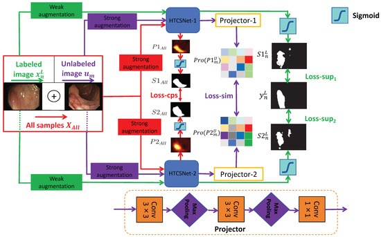
Figure 1. General structure of the proposed SSL framework (SemiPolypSeg).

Consider the labeled set $X_n^L$ = $\{(x_1^L,y_1^L),\dots ,(x_n^L,y_n^L)\}$, where each pair $(x_i^L,y_i^L)$ includes an image $x_i^L\in {\mathbb{R}}^{C\times H\times W}$ and its corresponding ground truth mask $y_i^L\in {\{0,1\}}^{H\times W}$. Additionally, let $X_m^U={\left\{u_i\right\}}_{i=1}^m$ represent a set of m unlabeled images, where $u_i\in {\mathbb{R}}^{C\times H\times W}$ and $m\gg n$. The main objective is to develop a segmentation model using the combined dataset $X_{All}$ = $(X_n^L\cup X_m^U)$. Throughout the training process, the entire dataset $X_{\mathrm{All}}$ undergoes various perturbations for both weak and strong data augmentation. The augmented labeled and unlabeled data are subsequently fed into HTCSNet-1 and HTCSNet-2, with each initialized using distinct parameters, to independently generate their predictions. For additional contrastive learning, the predictions are input into projectors (projector-1 and projector-2) for all unlabeled data. During inference, we can input polyp images into any segmentation network model to achieve segmentation results without needing projectors.

Our study introduces a novel loss function composed of supervised segmentation loss, feature consistency loss (CPS loss), and patch-wise contrastive loss (similarity loss)—aimed at enhancing model convergence. $X_n^L$ with weak data augmentation, including rotations and flips, are input to HTCSNet-1 and HTCSNet-2, computing $P{1}_n^L$ and $P{2}_n^L$. We then apply the activation function (sigmoid) to generate the respective polyp segmentation outputs maps $S{1}_n^L$ and $S{2}_n^L$. The supervised losses for HTCSNet-1 and HTCSNet-2 are determined by the differences between $S{1}_n^L$, $S{2}_n^L$, and $Y_n^L$. After undergoing strong data augmentation, including rotations, flips, affine transformations, random grayscale noise, Gaussian blur, color jittering, and GridMask [62], $X_{All}$ is fed into different segmentation networks. This process generates the corresponding polyp probability distribution predictions $P{1}_{All}$ and $P{2}_{All}$. The polyp segmentation maps $S{1}_{All}$ and $S{2}_{All}$ are derived from $P{1}_{All}$ and $P{2}_{All}$ using the sigmoid activation function. These maps, $S{1}_{All}$ and $S{2}_{All}$, serve as pseudo-labels and are compared to calculate the CPS loss for both networks.

All unlabeled images $X_m^U$ with strong data augmentation are fed into HTCSNet-1 and HTCSNet-2 to obtain $P{1}_m^U$ and $P{2}_m^U$. Then, the feature representations Pro($P{1}_m^U$) and Pro($P{2}_m^U$) are extracted through projector modules ${\left\{Pr{o}_i(·)\right\}}_{i=1}^2$. Finally, patch-wise contrastive loss is employed to maximize feature variations at disparate spatial locations and minimize feature variations at matching spatial locations between Pro($P{1}_m^U$) and Pro($P{2}_m^U$). We outline the detailed methodology in the subsequent sections.

3.2. Hybrid Transformer–CNN Segmentation Networks

CNN segmentation networks excel at extracting local features but struggle to capture global representations, limiting their performance in complex segmentation tasks. Compared to CNNs, transformers utilize embedding and self-attention mechanisms, which are very efficient in gathering global information and dealing with long-distance dependencies. Recent studies have shown that a hybrid dual-encoder architecture can significantly improve feature learning for precise image segmentation [15,44]. This study introduces HTCSNet, a novel deep learning segmentation network that integrates CNN and transformer encoders for polyp segmentation. HTCSNet not only excels in local feature extraction but also effectively captures global semantic information.

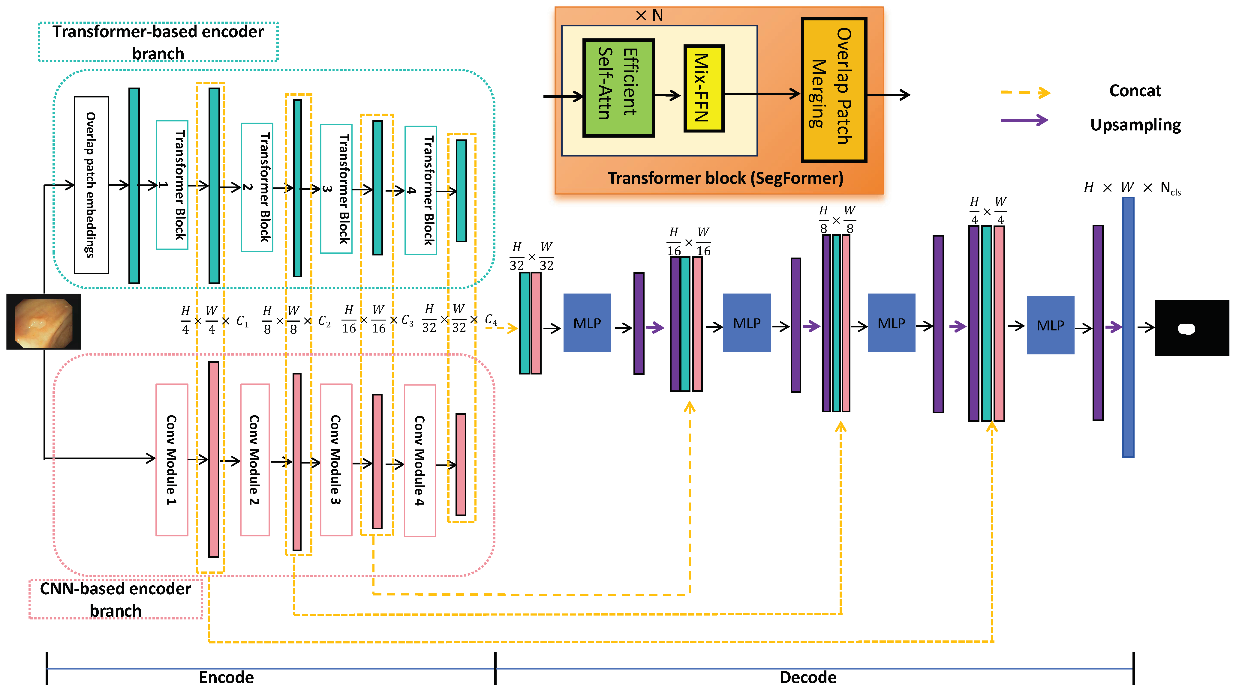
As illustrated in Figure 2, HTCSNet consists of three main components: a CNN-based encoder branch, a transformer-based encoder branch, and an ALL-MLP decoder. By integrating the CNN and transformer in the encoder, the data requirements for the transformer network are significantly reduced. During the decoding stage, feature fusion with MLP and skip connections leverages the strengths of both branches, enhancing learning capabilities. The following sections provide a detailed explanation of these three components.

Figure 2. General structure of the proposed HTCSNet.

3.2.1. CNN-Based Encoder Branch

The convolutional neural network serves as a robust, fine-grained feature extractor, making it adept at identifying unique local polyp features. In our study, we strategically leverage the encoder of Res2Net-101 [63] as a CNN encoding branch. This particular model is pretrained on the vast ImageNet database, ensuring a strong foundation for feature extraction.

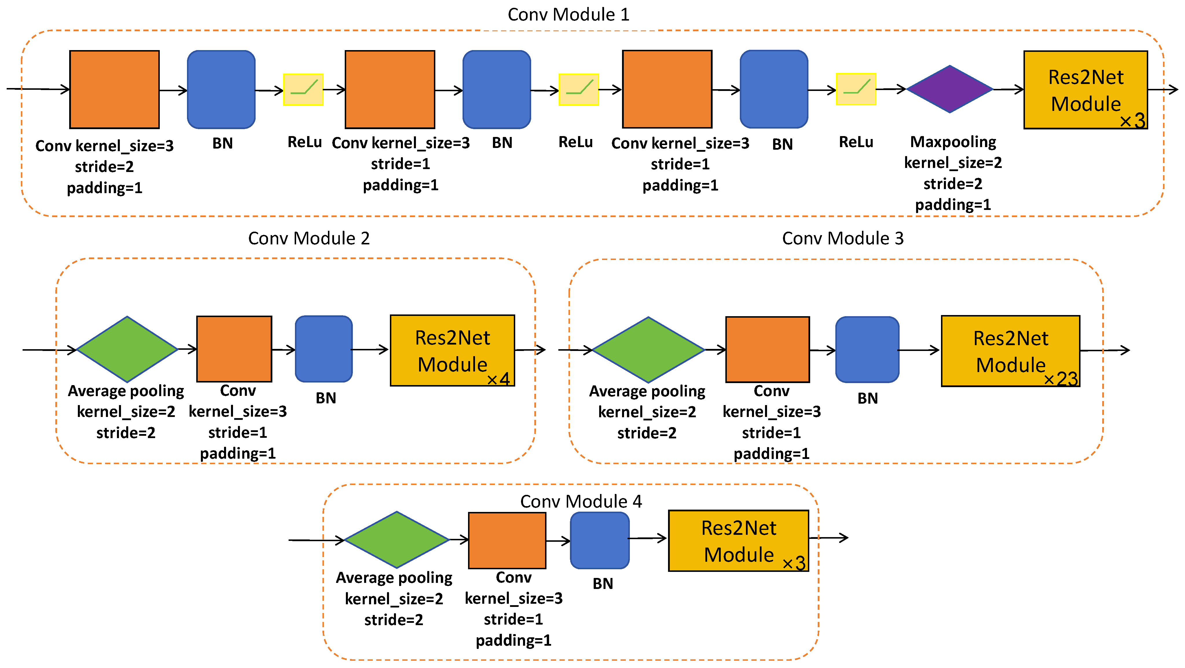
Res2Net-101 is a sophisticated network architecture, which has been expertly designed to efficiently extract hierarchical local features $F_{ci}$ $(i=1,2,3,4)$ at multiple resolutions $\{{\displaystyle \frac{1}{4}},{\displaystyle \frac{1}{8}},{\displaystyle \frac{1}{16}},{\displaystyle \frac{1}{32}}\}$ of the original image size. This is made possible through a series of meticulously designed convolutional modules (please refer to Figure 3 and Figure 4) equipped with skip connections. The CNN-based encoder branch, through its progressive feature extraction, precisely captures local semantic details from the original polyp image, providing a rich source of features for subsequent analysis.

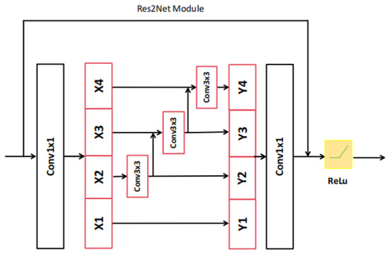
Figure 3. The architecture of Res2Net module.

Figure 4. The architecture of designed convolutional modules.

3.2.2. Transformer-Based Encoder Branch

The transformer-based encoder extracts global features from polyp images by utilizing the self-attention mechanism to model input–output dependencies. We leverage the SegFormer encoder [64], pretrained on ImageNet, as the transformer-based encoder branch. SegFormer is a sophisticated structure, which is theoretically elegant and practically efficient. It achieves competitive performance with significantly fewer parameters than traditional convolutional neural networks. SegFormer segments the input image into overlapping patches, embedding these into a sequence of vectors. The architecture is meticulously designed to process these embeddings through a series of hierarchical Transformer blocks, extracting a multiscale representation $F_{ti}$ $(i=1,2,3,4)$ at resolutions of $\{{\displaystyle \frac{1}{4}},{\displaystyle \frac{1}{8}},{\displaystyle \frac{1}{16}},{\displaystyle \frac{1}{32}}\}$ of the original image size and capturing both fine details and broader context.

3.2.3. ALL-MLP Decoder

The final component of HTCSNet is the ALL-MLP decoder, which facilitates the fusion of the hierarchical features $F_{ci}$, $(i=1,2,3,4)$, and $F_{ti}$ $(i=1,2,3,4)$ derived from both the CNN-based and transformer-based encoder branches to achieve the final polyp segmentation map. This decoder adopts a structure that resembles the UNet architecture, with a series of upsampling and concatenation operations that facilitate the integration of multiscale features. The concatenated features from the CNN and transformer branches are fused through a series of MLP layers, which serve as a way for the global and local features’ fusion. This fusion results in a comprehensive feature representation $F_{fi}$ $(i=1,2,3,4)$ that encapsulates both the fine-grained details and the broader context of the polyp image. The ALL-MLP decoder employs bilinear upsampling to gradually upscale the fused features $F_{fi}$ $(i=1,2,3,4)$, aligning them with the original image dimensions. At each upsampling stage, the decoder concatenates the upscaled features with the corresponding features from the encoder branches, which are further enriched by the MLP-based fusion. This iterative process culminates in the generation of the final segmentation map S, which is produced by upsampling $F_{f1}$ and concatenating it with the shallowest features $F_{c1}$ and $F_{t1}$, followed by an MLP layer that refines the segmentation outcome. Finally, semantic segmentation of the image is performed.

3.3. Cross-Pseudo Supervision and Contrastive Learning

The SemiPolypSeg framework innovatively merges cross-pseudo supervision and patch-wise contrastive learning within the training regimen, significantly diminishing the dependency on extensive labeled datasets. Moreover, it curtails the overreliance on contextual cues, concurrently enhancing the assimilation of global information.

CPS is operationalized by controlling the outputs of two structurally identical segmentation networks that differ in their parameter initialization. The iterative training process, enriched with data perturbations, mandates consistency in the outputs for identical inputs across both models. These networks concurrently generate segmentation predictions, serving as pseudo-labels for each other. Subsequently, these pseudo-labels are employed as supervisory signals for the unlabeled data, fostering a robust learning environment.

In the proposed framework, the model applies contrastive learning to train with diverse sample pairs, including both positive and negative ones. Positive pairs are formed from similar samples, while negative pairs consist of dissimilar ones. High-level features of a given image should remain invariant to feature transformation, being distinct across various spatial locations yet consistent at the same location within an image. Patch-wise contrastive learning aims to minimize patch-wise contrastive loss by leveraging an extensive dataset of unlabeled data. The architecture of the projector is constructed with convolutional layers of $3\times 3$ kernel size and max pooling layers with $2\times 2$ filters, which are arranged in three stages. These are subsequently linked to a convolutional layer with a $1\times 1$ kernel size. Each polyp image undergoes an initial transformation through two segmentation models with different initializations. The projector should yield identical feature representations for similar images. To identify feature similarities, suitable contrastive loss functions are employed. In particular, the projectors (projector-1 and projector-2) process an unlabeled image, which has been converted into two unique probability distribution maps by the HTCSNet-1 and HTCSNet-2, aiming to extract high-level semantic information that remains consistent across both maps. The projector generates various sample pairs, including positive and negative ones. Positive pairs have the same features at the same spatial positions, while negative pairs have different features at different positions. Through iterative training, the objective is to minimize patch-wise contrastive loss, thereby improving segmentation accuracy.

3.4. Loss Function

In this study, we use a hybrid loss function that consists of three components: supervised training losses for both segmentation models(HTCSNet-1 and HTCSNet-2) using labeled data (Loss-sup), CPS loss applied to all data (Loss-cps), and contrastive learning loss for unlabeled data (Loss-sim). For the supervised training losses using labeled data, the outputs from the HTCSNet-1 and HTCSNet-2 are matched against the ground truth to calculate ${\mathrm{Loss}\text{-}\sup }_1$ and ${\mathrm{Loss}\text{-}\sup }_2$. These losses are computed using a composite loss, which integrates a weighted Intersection over Union (IoU) loss and a weighted Binary Cross-Entropy (BCE) loss. The supervised training loss is defined as in Equations (1)–(3).

$${\mathrm{Loss}\text{-}\sup }_1={\mathrm{Loss}}_{{\mathrm{IoU}}_1}^{\mathrm{w}}+{\mathrm{Loss}}_{{\mathrm{BCE}}_1}^{\mathrm{w}}$$

(1)

$${\mathrm{Loss}\text{-}\sup }_2={\mathrm{Loss}}_{{\mathrm{IoU}}_2}^{\mathrm{w}}+{\mathrm{Loss}}_{{\mathrm{BCE}}_2}^{\mathrm{w}}$$

(2)

$$\mathrm{Loss}\text{-}\sup ={\mathrm{Loss}\text{-}\sup }_1+{\mathrm{Loss}\text{-}\sup }_2$$

(3)

For the CPS loss, all data are fed into two models, each followed by a sigmoid activation function, to obtain their respective segmentation predictions as pseudo-labels ($S_i$(i = 1,2)), which can be used as a supervisory signal for the other network. Different from the supervised training losses, the cross-pseudo supervision loss (Loss-cps)uses cross-pseudo-labels of both networks as the true labels. Loss-cps can also be determined by combining a weighted IoU loss with a weighted BCE loss. Loss-cps is calculated as in Equations (4)–(6).

$${\mathrm{Loss}\text{-}\mathrm{cps}}_1={({\mathrm{Loss}}_{{\mathrm{IoU}}_1}^{\mathrm{w}}+{\mathrm{Loss}}_{{\mathrm{BCE}}_1}^{\mathrm{w}})}_{{\mathrm{S}}_2}$$

(4)

$${\mathrm{Loss}\text{-}\mathrm{cps}}_2={({\mathrm{Loss}}_{{\mathrm{IoU}}_2}^{\mathrm{w}}+{\mathrm{Loss}}_{{\mathrm{BCE}}_2}^{\mathrm{w}})}_{{\mathrm{S}}_1}$$

(5)

$$\mathrm{Loss}\text{-}\mathrm{cps}={\mathrm{Loss}\text{-}\mathrm{cps}}_1+{\mathrm{Loss}\text{-}\mathrm{cps}}_2$$

(6)

In the context of patch-wise contrastive learning, unlabeled data are fed into two distinct models, HTCNet-1 and HTCNet-2, to generate polyp distribution maps. These maps are then processed by projectors to obtain high-level semantic representations of the polyp images. When the same polyp image is transformed using both HTCNet-1, HTCNet-2, as well as two projectors, the high-level features produced are expected to be consistent. Therefore, patch-wise contrastive loss (Loss-sim) is employed to measure their similarity, with the calculation of Loss-sim detailed in Equation (7).

$$\mathrm{Loss}\text{-}\mathrm{sim}=-log{\displaystyle \frac{exp(\mathrm{p}·{\mathrm{p}}^{+}/\tau )}{exp(\mathrm{p}·{\mathrm{p}}^{+}/\tau )+\sum exp(\mathrm{p}·{\mathrm{p}}^{-}/\tau )}}$$

(7)

Here, ($\mathrm{p}·{\mathrm{p}}^{+}$) and ($\mathrm{p}·{\mathrm{p}}^{-}$) denote positive and negative sample pairs, respectively, representing feature representations from projector-1 and projector-2 at the same position and at different positions. In the experiments, we set $\tau$ as the temperature coefficient to 0.07.

The SemiPolypSeg framework, designed for the segmentation of polyps, harnesses the power of both labeled and unlabeled data for learning. For the labeled data, the loss is composed of the supervised training loss and the cross-pseudo supervision loss; For the unlabeled data, the loss is composed of the contrastive learning loss and the CPS loss. By progressively minimizing the total loss using gradient descent throughout the training process, the model achieves optimal segmentation performance. The total loss (Loss-Total) is determined by Equation (8).

$$\mathrm{Loss}\text{-}\mathrm{Total}=\lambda ·\mathrm{Loss}\text{-}\sup +\beta ·\mathrm{Loss}\text{-}\mathrm{cps}+\gamma ·\mathrm{Loss}\text{-}\mathrm{sim}$$

(8)

where $\lambda$, $\beta$, and $\gamma$ are the weights of the supervised training losses, the cross-pseudo supervision loss, and the patch-wise contrastive learning loss, which are hype parameters.

Considering the importance and scarcity of labeled data, we assigned a higher weight ($\lambda$) to the supervised loss to ensure that the model effectively leverages this valuable resource, which is crucial for learning accurate representations. Based on experience, supervised learning, when combined with semi-supervised methods, often requires a higher emphasis on labeled data to guide the learning process effectively. The CPS loss ($\beta$) and contrastive learning loss ($\gamma$) were given equal weights to balance their contributions, as both are essential for utilizing the unlabeled data to improve the model’s generalization. This balanced approach ensures that the model benefits from both labeled and unlabeled data, leading to better overall performance. Therefore, in our experiments, we chose $\lambda$ to be 0.4, $\beta$ to be 0.3, and $\gamma$ to be 0.3. The complete SemiPolypSeg optimization process is outlined in Algorithm 1.

Algorithm 1 SemiPolypSeg (training)

Input: Define the segmentation networks ${\left\{HTCSNe{t}_i(·)\right\}}_{i=1}^2$, projectors ${\left\{Pr{o}_i(·)\right\}}_{i=1}^2$, batch size B, maximum epoch $Epoc{h}_{\max }$, labeled images $X_n^L={\left\{(x_i^L,y_i^L)\right\}}_{i=1}^n$, unlabeled images $X_m^U={\left\{u_i\right\}}_{i=n+1}^m$, and all datasets $X_{\mathrm{All}}=X_n^L\cup X_m^U$. Parameter: ${\left\{{\theta }_i\right\}}_{i=1}^2$ of ${\left\{HTCSNe{t}_i(·)\right\}}_{i=1}^2$ Output: ${\left\{HTCSNe{t}_i(·;{\theta }_i)\right\}}_{i=1}^2$. Initialization: Initialize network and projector parameters ${\left\{{\theta }_i\right\}}_{i=1}^2$ and ${\left\{{\mu }_i\right\}}_{i=1}^2$.  1: for epoch = 1 to $Epoc{h}_{\max }$ do  2:     for all batches B do  3:         Generate predictions for labeled data $HTCSNe{t}_1\left(x_i^L\right)$ and $HTCSNe{t}_2\left(x_i^L\right)$ for all $x_i^L\in X_n^L$;  4:         Generate predictions for unlabeled data $HTCSNe{t}_1\left(u_i\right)$ and $HTCSNe{t}_2\left(u_i\right)$ for all $u_i\in X_m^U$  5:         for all $u_i\in X_m^U$, Generate feature maps $Pr{o}_1\left(HTCSNe{t}_1\left(u_i\right)\right)$ and $Pr{o}_2\left(HTCSNe{t}_2\left(u_i\right)\right)$ from two projectors.  6:         Let $\mathrm{Loss}\text{-}\mathrm{Total}=\lambda ·\mathrm{Loss}\text{-}\sup +\beta ·\mathrm{Loss}\text{-}\mathrm{cps}+\gamma ·\mathrm{Loss}\text{-}\mathrm{sim}$, as defined in Equations (1)–(8).  7:         Update ${\left\{{\theta }_i\right\}}_{i=1}^2$ by applying gradient descent on Loss-Total.  8:     end for  9: end for return ${\left\{HTCSNe{t}_i(·;{\theta }_i)\right\}}_{i=1}^2$.

4. Results

We performed experiments to benchmark our approach against other semi-supervised segmentation methods on two public polyp segmentation datasets. Additionally, we carried out ablation studies to test the effectiveness of each component of our approach.

4.1. Datasets and Evaluation Metrics

The datasets utilized in our experiments were chosen for their diversity and relevance to polyp segmentation, enabling a thorough evaluation of our method’s performance.

Our approach was evaluated on two widely recognized polyp segmentation datasets: Kvasir-SEG [65] and CVC-ClinicDB [66]. The Kvasir-SEG dataset includes 1000 images with dimensions that vary from 332 × 487 pixels to 1920 × 1072 pixels. The CVC-ClinicDB dataset contains 612 images, each with a resolution of 384 × 288 pixels. Prior to training, we standardized the image sizes from both datasets to 256 × 256 pixels to ensure uniformity in the input data. In our experiments, we adhered to the training settings outlined in the existing literature [67], which similarly divided the two datasets. We randomly selected 80% of the images for training, 10% for validation, and 10% for testing. In the training phase, a mere 15% and 30% of the images were designated as labeled data, while the rest were utilized as unlabeled data. Table 2 enumerates the image size of these datasets and specifies the number of images allocated to the training, validation, and test sets.

Table 2. The description of Kvasir and CVC-ClinicDB datasets.

Datasets	Number of Images	Size	Train	Valid	Test
Kvasir-SEG [65]	1000	Variable	800	100	100
CV-ClinicDB [66]	612	384 × 288	488	62	62

Segmentation performance was evaluated using the dice similarity coefficient (DSC), which is commonly employed for the quantitative assessment of polyp segmentation. The calculation formula is given in Equation (9).

$$\mathrm{DSC}={\displaystyle \frac{2TP}{2TP+FP+FN}}$$

(9)

4.2. Implementation Details

Our SemiPolypSeg has been developed using the PyTorch 1.8.0 framework, with an NVIDIA RTX 3090 GPU. For parameter optimization during training, we utilized the AdamW optimizer [68], which is a variant of the Adam optimizer with improved regularization, and its parameters are listed in the Table 3, including the initial learning rate (Lr), coefficient (${\beta }_1$,${\beta }_2$) used for computing running averages of the gradient and its square, and the weight decay. The training process consisted of 300 epochs, incorporating an early stopping strategy that halted the training if the model showed no improvement in the validation set for 50 consecutive epochs. We dynamically adjusted the learning rate using a poly strategy, multiplying the initial learning rate by ${\left(1-{\displaystyle \frac{epoch}{max-epoch}}\right)}^{0.9}$.

Table 3. The parameters of the AdamW optimizer.

Lr	${\mathit{\beta }}_1$	${\mathit{\beta }}_2$	Weight Decay
0.0001	0.9	0.999	0.0001

During SemiPolypSeg training, a portion of the training data was designated as labeled based on the experimental ratio, while the remainder was used as unlabeled data. For fair comparisons, we employed identical validation and test sets in all experiments. During the training phase, various weak and strong data augmentation techniques were employed, which enhanced the model’s ability to learn generalizable representations and increased the variety of the image samples, thereby reducing the risk of overfitting. A hybrid loss function was used as a guide to update the model parameters. After each training cycle, the DSC for the validation set was computed, and the model parameters that achieved the highest DSC were saved. During semi-supervised training, each batch comprised both labeled and unlabeled data, with two labeled and two unlabeled images included. For the fully supervised training, there was no change to the batch size.

4.3. Methods Comparison Analysis

In this section, we compare the proposed method SemiPolypSeg with other current SOTA semi-supervised algorithms under different partition protocols on Kvasir-SEG and CVC-ClinicDB, including mean teacher (MT) [20], Cross-Consistency Training (CCT) [21], CMT [19], and UCMT [19]. HTCSNet’s fully-supervised training, using only the specified proportion of labeled data, produced the baseline model. To establish a performance benchmark, HTCSNet underwent fully supervised training with 100% labeled data, delineating the upper limit of its capabilities. For the performance of alternative methods, we utilized the findings presented in the paper [19]. To ensure fair comparisons, our method was implemented using two segmentation networks: DeepLabv3+ and HTCSNet, respectively.

Table 4 presents the outcomes of comparative experiments on Kvasir-SEG under 15% and 30% labeled images. With 15% labeled images, the proposed SemiPolypSeg method with DeepLabv3+ architecture demonstrated consistent and significant advancements compared to other SOTA semi-supervised learning methods in terms of the DSC. By using 15% labeled images and 85% unlabeled images, the DSC increased by 1.59%, 7.89%, 0.95%, and 0.35% compared to MT, CCT, CMT, and UCMT, respectively. When using 30% labeled images, all semi-supervised learning methods showed improvement. Our approach still exhibited substantial performance gains, with the DSC increasing by 1.19%, 5.24%, 1.3%, and 0.85% compared to MT, CCT, CMT, and UCMT, respectively.

Table 4. Quantitative comparison of our method with other semi-supervised methods on Kvasir-SEG using 15% and 30% labeled data. Bold values highlight the top performance in comparison to other SOTA approaches.

Method	Labeled/Unlabeled	DSC (%)
Fully supervised (HTCSNet)	800/0	90.95
Baseline (supervised-only)	120/0	86.33
MT (DeepLabv3+) [20]	120/680	87.44
CCT (DeepLabv3+) [21]	120/680	81.14
CMT (DeepLabv3+) [19]	120/680	88.08
UCMT (DeepLabv3+) [19]	120/680	88.68
SemiPolypSeg (DeepLabv3+) (ours)	120/680	89.03
SemiPolypSeg (HTCSNet) (ours)	120/680	89.68
Baseline (supervised-only)	240/0	87.45
MT (DeepLabv3+) [20]	240/560	88.72
CCT (DeepLabv3+) [21]	240/560	84.67
CMT (DeepLabv3+) [19]	240/560	88.61
UCMT (DeepLabv3+) [19]	240/560	89.06
SemiPolypSeg (DeepLabv3+) (ours)	240/560	89.91
SemiPolypSeg (HTCSNet) (ours)	240/560	90.62

In addition, comparing the DeepLabv3+ architecture, we conducted experiments on Kvasir-SEG under 15% and 30% labeled images using the SemiPolypSeg framework with the HTCSNet architecture that is proposed in this paper. The results demonstrate our proposed new architecture (HTCSNet)’s effectiveness. Our method with HTCSNet obtained the highest DSC of 89.68% and 90.62%, outperforming the SemiPolypSeg framework with DeepLabv3+ architecture by 0.65% and 0.71%, respectively.

Table 5 presents the performance of our proposed method compared to other SOTA methods using 15% and 30% labeled images on CVC-ClinicDB. Similarly, our method achieved the top performance with the highest DSC of 89.72% and 90.06% for 15% and 30% labeled data, respectively. It outperformed other approaches (MT, CCT, CMT, and UCMT) by 5.21% (5.28%), 11.15% (15.27%), 2.78% (3.59%), and 2.1% (2.17%) for 15% (30%) labeled data, respectively. Through experiments on these two datasets, we can find that our method significantly improves performance with limited labeled data compared to other methods. This indicates that it can more efficiently utilize unlabeled images than other semi-supervised methods.

Table 5. Quantitative comparison of our method with other semi-supervised methods on CVC-ClinicDB using 15% and 30% labeled data. Bold values highlight the top performance in comparison to other SOTA approaches.

Method	Labeled/Unlabeled	DSC (%)
Fully supervised (HTCSNet)	488/0	90.90
Baseline (supervised-only)	74/0	85.16
MT (DeepLabv3+) [20]	74/414	84.19
CCT (DeepLabv3+) [21]	74/414	74.20
CMT (DeepLabv3+) [19]	74/414	85.88
UCMT (DeepLabv3+) [19]	74/414	87.30
SemiPolypSeg (DeepLabv3+) (ours)	74/414	89.47
SemiPolypSeg (HTCSNet) (ours)	74/414	89.72
Baselinen(supervised-only)	148/0	86.38
MT (DeepLabv3+) [20]	148/340	84.40
CCT (DeepLabv3+) [21]	148/340	78.46
CMT (DeepLabv3+) [19]	148/340	86.83
UCMT (DeepLabv3+) [19]	148/340	87.51
SemiPolypSeg (DeepLabv3+) (ours)	148/340	89.61
SemiPolypSeg (HTCSNet) (ours)	148/340	90.06

4.4. Ablation Experiments

To illustrate the impact of each component in SemiPolypSeg, we conducted four distinct experiments: training HTCSNet by adding only CPS, training by adding only contrastive learning, training without the transformer encoder branch (w/o Transformer), and training without the CNN encoder branch (w/o CNN). The CVC-ClinicDB dataset, with only 15% labeled data, was used to evaluate segmentation performance using the DSC metric. Table 6 presents the DSC findings from all experiments, indicating that SemiPolypSeg surpassed other frameworks, showing a mean enhancement of 1.62% over CPS alone and 4.43% over contrastive learning alone. Using HTCSNet with dual-encoder branches led to an average improvement of 3.99% and 5.48% compared to networks without the transformer encoder branch and without the CNN encoder branch, respectively, highlighting its effectiveness in enhancing segmentation performance.

Table 6. Ablation study of various component combinations using just 15% labeled data on the CVC-ClinicDB dataset. HTCSNet: Hybrid Transformer–CNN Segmentation Network, serving as the baseline with only supervised training; Loss-sup: supervised training; Loss-cps: cross-pseudo supervision; Loss-sim: contrastive learning.

Network	Loss-sup	Loss-sim	Loss-cps	DSC
HTCSNet (baseline)	✓			85.16
HTCSNet	✓	✓		85.29
HTCSNet	✓		✓	88.10
HTCSNet (w/o CNN)	✓	✓	✓	84.24
HTCSNet (w/o Transformer)	✓	✓	✓	85.73
HTCSNet	✓	✓	✓	89.72

5. Discussion

5.1. Evaluation of Training and Validation Performance

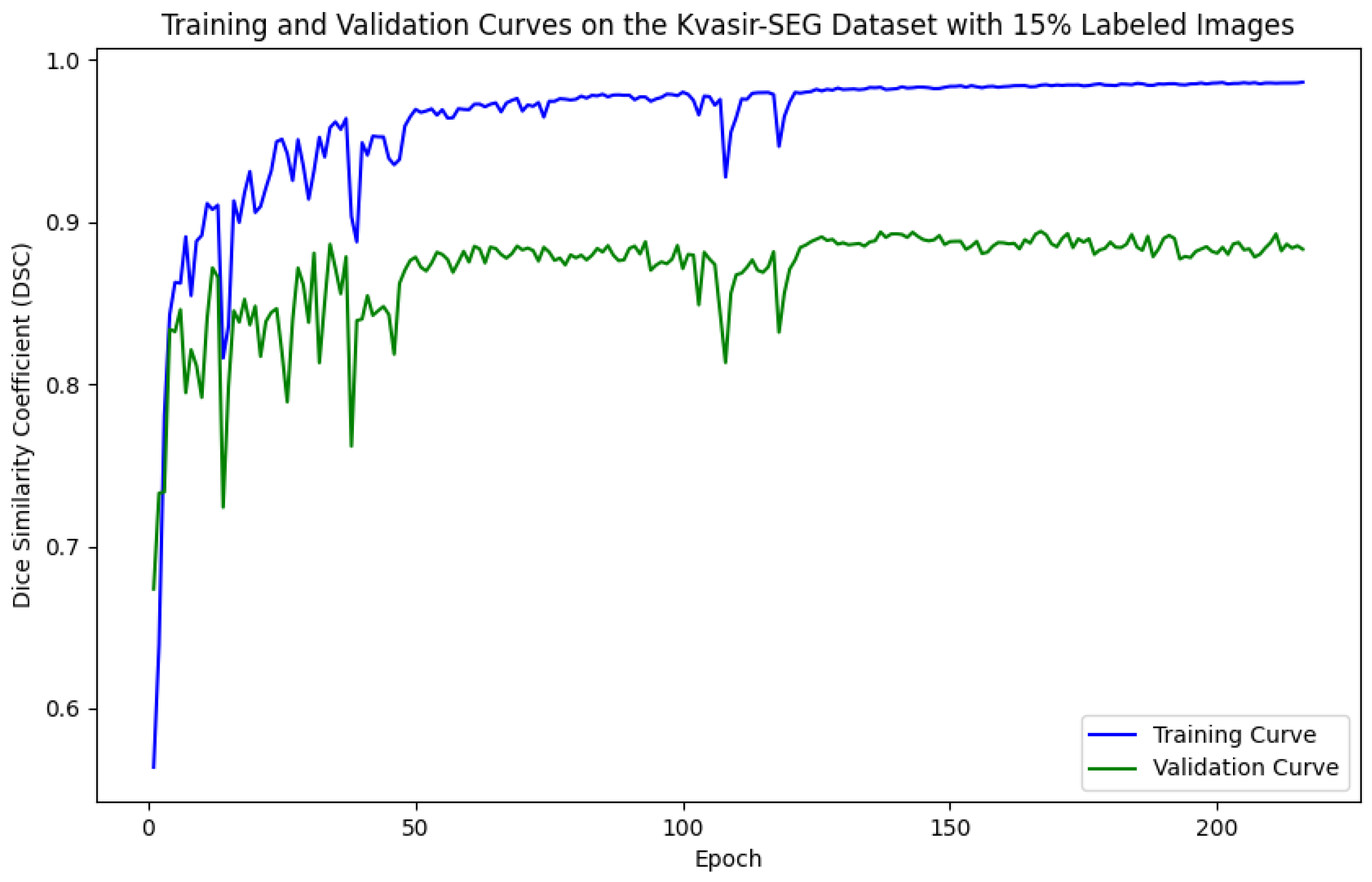
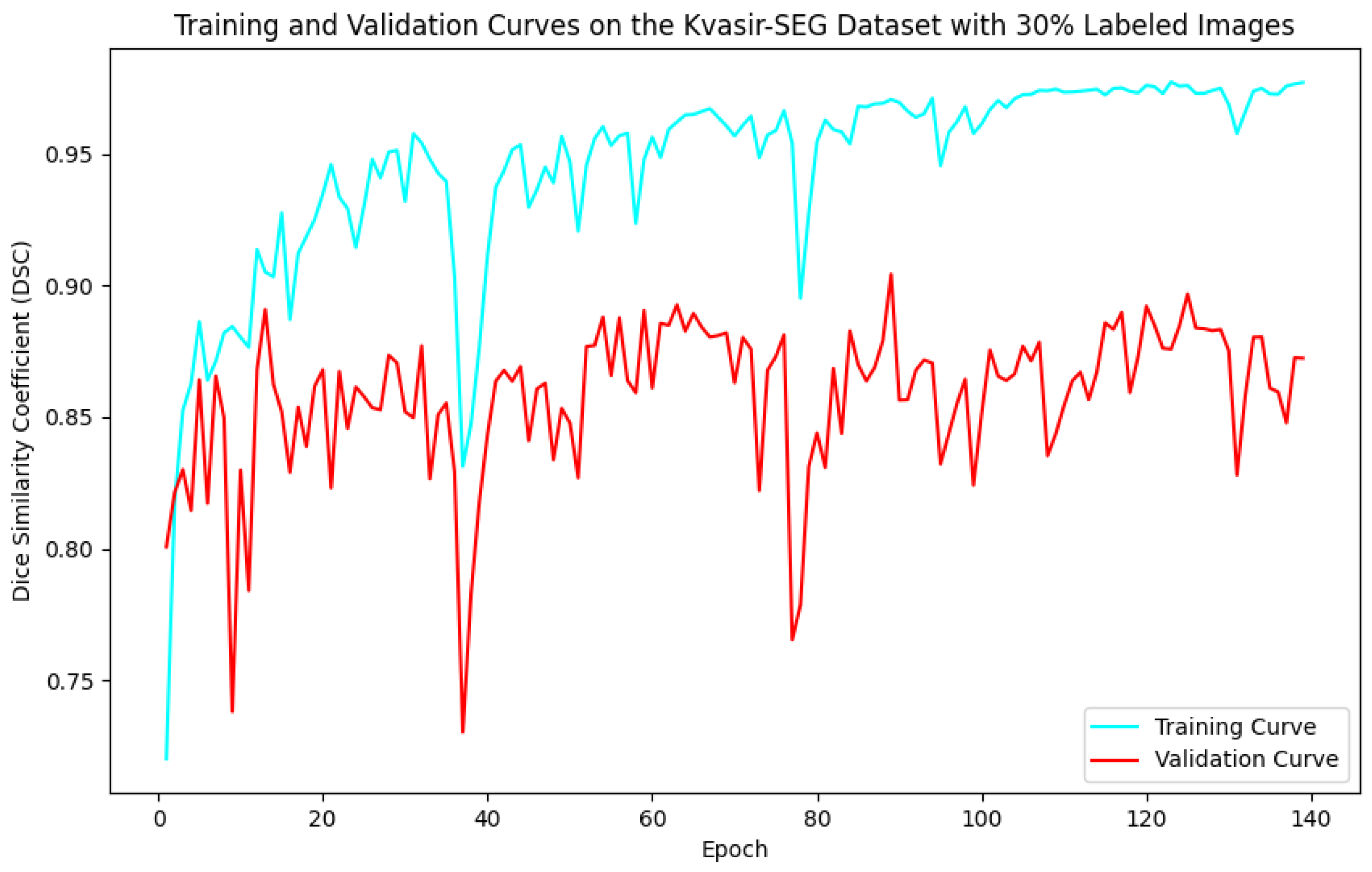
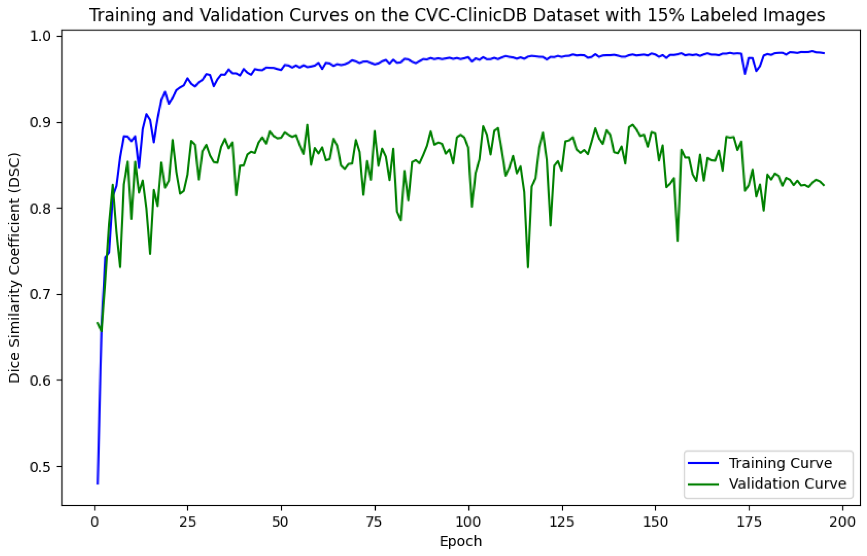
As illustrated in Figure 5, Figure 6, Figure 7 and Figure 8, the training and validation curves for the DSC criterion are presented as a function of the number of epochs on the Kvasir-SEG and CVC-ClinicDB datasets. Figure 5 and Figure 6 correspond to the Kvasir-SEG dataset with 15% and 30% labeled images, respectively, while Figure 7 and Figure 8 correspond to the CVC-ClinicDB dataset with 15% and 30% labeled images.

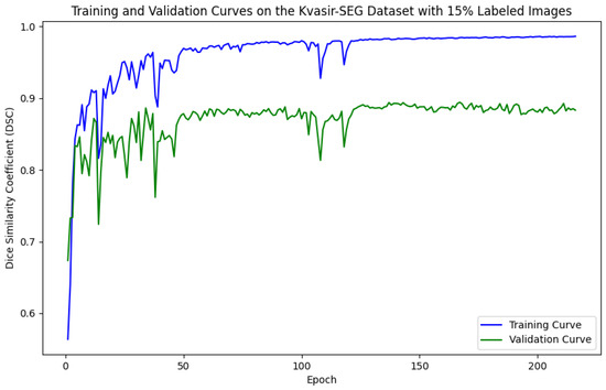
Figure 5. Training and validation curves for the DSC criterion as a function of the number of epochs on Kvasir-SEG with 15% labeled images. Dark blue denotes the training curve, while orange highlights the validation curve.

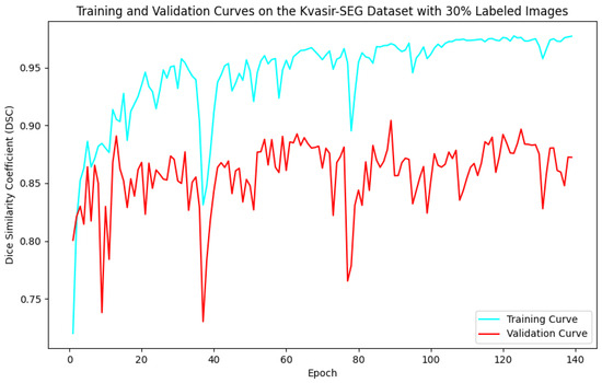
Figure 6. Training and validation curves for the DSC criterion as a function of the number of epochs on Kvasir-SEG with 30% labeled images. Dark blue denotes the training curve, while orange highlights the validation curve.

Figure 7. Training and validation curves for the DSC criterion as a function of the number of epochs on CVC-ClinicDB with 15% labeled images. Dark blue denotes the training curve, while orange highlights the validation curve.

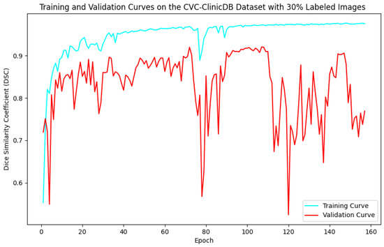
Figure 8. Training and validation curves for the DSC criterion as a function of the number of epochs on CVC-ClinicDB with 30% labeled images. Dark blue denotes the training curve, while orange highlights the validation curve.

The training process was designed to run for up to 300 epochs, incorporating an early-stopping strategy that halted training if the model showed no improvement over 50 continuous epochs on the validation set. This strategy was crucial in preventing overfitting by stopping the training once the model’s performance plateaued, ensuring the model did not learn noise from the training data. By stopping early, we achieved a model that balanced underfitting and overfitting, performing well on unseen data.

For the Kvasir-SEG dataset, as shown in Figure 5, the maximum number of training epochs was 216, with a maximum validation DSC of 89.41%, while Figure 6 shows 139 epochs with a maximum validation DSC of 90.43%. For the CVC-ClinicDB dataset, Figure 7 indicates 195 epochs with a maximum validation DSC of 89.78%, and Figure 8 shows 157 epochs with a maximum validation DSC of 91.96%. This evidence suggests that the chosen maximum training epoch parameter in our experiments is well-suited.

The performance dynamics of the segmentation model vary considerably depending on the quantity of labeled data available. As the proportion of labeled data increased, the segmentation model’s performance on the validation set improved, as demonstrated by higher DSC scores. Furthermore, it is evident that with more labeled data, the required number of training epochs decreased substantially. This indicates that as the amount of labeled data grows, the model converges more rapidly, leading to earlier termination of training and a reduction in the number of iterations. These findings highlight the critical role of labeled data in developing effective semi-supervised segmentation models and demonstrate the benefits of leveraging additional labeled data to achieve better results.

5.2. Qualitative Results Analysis

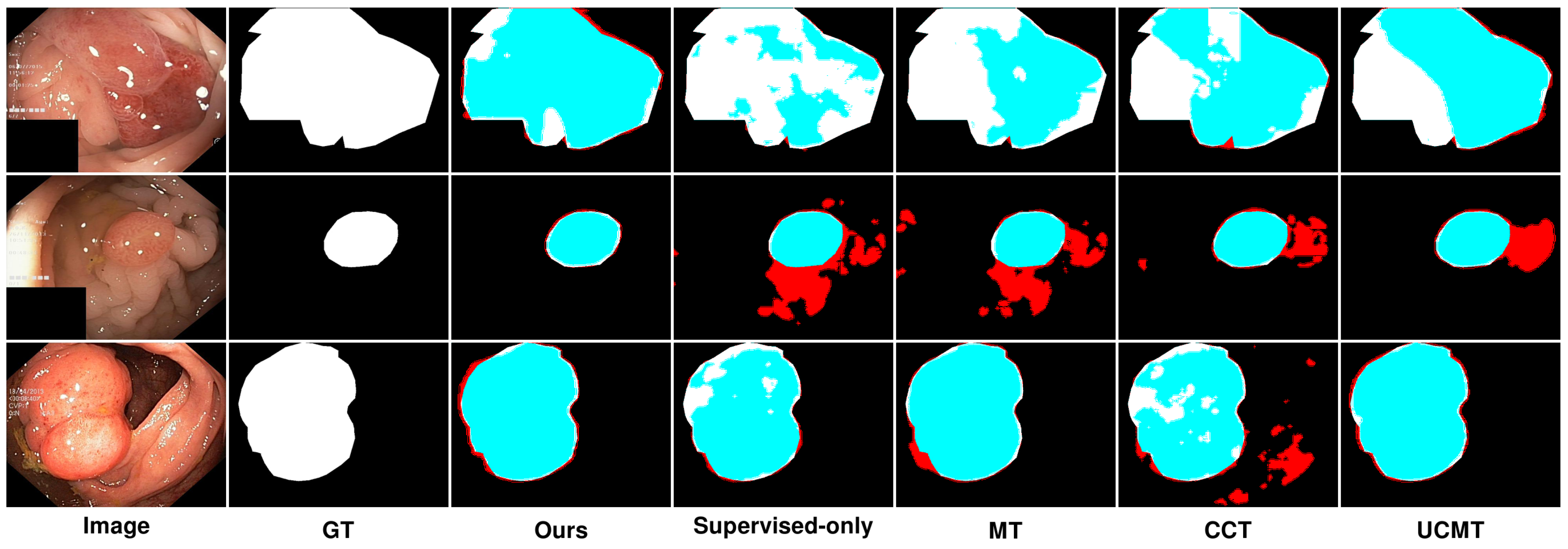
As presented in Figure 9 and Figure 10, the segmentation results predicted by the proposed SemiPolypSeg and other approaches using 15% labeled images on the Kvasir-SEG and CVC-ClinicDB datasets are provided. The baseline model (supervised-only), trained with fully supervised learning using only 15% of labeled data, shows the least accurate segmentation. The results are more fragmented and less reliable, highlighting the limitations of relying solely on labeled data. In contrast, the other semi-supervised segmentation methods, including MT, CCT, UCMT, and our proposed SemiPolypSeg, not only utilized the same proportion of labeled data but also leveraged the information from unlabeled data, resulting in better segmentation accuracy compared to the baseline.

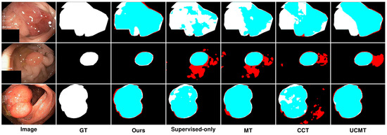
Figure 9. Qualitative results of different methods on Kvasir-SEG. Blue denotes the regions where the prediction aligns with the ground truth, while red highlights the areas where the prediction diverges from the ground truth.

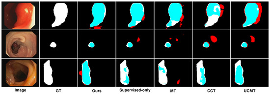
Figure 10. Qualitative results of different methods on CVC-ClinicDB. Blue denotes the regions where the prediction aligns with the ground truth, while red highlights the areas where the prediction diverges from the ground truth.

In Figure 9, we can see that on the Kvasir-SEG dataset, using 15% labeled images, the segmentation performance varied across different methods. While MT showed reasonable segmentation, it often struggled with accurately capturing the finer details of the polyp boundaries, resulting in less precise segmentation, with some areas showing over-segmentation or under-segmentation. Although the method’s reliance on consistency between teacher and student models helped, it was not sufficient for complex polyp shapes. In contrast, CCT provided better segmentation than MT, with improved edge detection and overall segmentation quality; however, it still fell short in terms of edge smoothness and overlap with the ground truth. The segmentation results were less consistent, especially in regions with complex textures or irregular shapes. Similarly, UCMT performed comparably to CCT but tended to produce noisier segmentation results, with more irregular edges and occasional misclassifications. This method benefited from unsupervised consistency but struggled with maintaining smooth and accurate boundaries. On the other hand, SemiPolypSeg achieved more accurate delineation of polyp boundaries, reducing false positives and negatives. The method’s ability to maintain the integrity of the polyp shape, even with limited labeled data, highlights its robustness and effectiveness. Consequently, the segmentation results are smoother and show a higher overlap with the ground truth, particularly at the lesion edges.

Similarly, Figure 10 presents the results on the CVC-ClinicDB dataset, highlighting comparable trends with some dataset-specific observations. On the CVC-ClinicDB dataset, MT again showed reasonable performance but lacked the precision and smoothness of SemiPolypSeg. The segmentation results are less accurate, particularly at the lesion edges, where MT struggled to capture the fine details. Although CCT provided better segmentation than MT, with improved edge detection and overall segmentation quality, it still exhibited some inconsistencies, especially in areas with complex textures. The method showed better performance than MT but was still not as smooth or accurate as SemiPolypSeg. Similarly, UCMT’s performance is comparable to CCT, with slightly better edge detection but more noise in the segmentation results. While the method showed some improvement in capturing the lesion boundaries, it still produced irregular edges and occasional misclassifications. On the other hand, SemiPolypSeg outperformed other methods by providing clearer and more precise segmentation. The edges of the lesions are more accurately captured, which is crucial for clinical applications where precise boundary detection is necessary for diagnosis and treatment planning. The method showed consistent and reliable segmentation across different regions of the dataset, highlighting its effectiveness in leveraging both labeled and unlabeled data.

In summary, the qualitative experimental results in our study indicate that under conditions with a small proportion of labeled samples, semi-supervised segmentation methods outperform fully supervised methods. This is because semi-supervised methods not only use labeled data as a supervisory signal but also exploit the internal information of unlabeled data, enhancing the model’s learning performance and generalization ability. Compared to other semi-supervised approaches, SemiPolypSeg (Ours) showed better segmentation performance, with a higher overlap with the ground truth and smoother segmentation results at the lesion edges. We attribute this to two main factors:

Firstly, the HTCSNet architecture combines the advantages of CNNs for capturing local details and transformers for global modeling, significantly enhancing effective image semantic representation. Secondly, compared to other methods, SemiPolypSeg effectively leverages CPS loss and patch-wise contrastive loss to learn semantic features from unlabeled images, improving the model’s learning ability and generalization performance. CPS loss ensures prediction consistency, while contrastive loss further enhances the utilization of unlabeled images by imposing feature similarity constraints between positive and negative sample pairs. The combination of these two losses enhances model performance while diminishing the dependence on extensively labeled datasets. Ablation studies in this research also demonstrate the effectiveness of each module of our method.

6. Conclusions

The labor-intensive nature of manual polyp image labeling makes it challenging to use fully supervised deep learning methods for polyp segmentation tasks that require large amounts of labeled data. In response, we introduce SemiPolypSeg, a semi-supervised segmentation framework that leverages cross-pseudo supervision and contrastive learning, thereby reducing the need for extensive labeled data. By learning from a broader set of unlabeled polyp images, this framework significantly reduces dependency on labeled images, thereby boosting model efficacy. Rigorous testing on the Kvasir-SEG and CVC-ClinicDB datasets confirms our framework’s superiority, outperforming other leading semi-supervised algorithms with only a small amount of labeled images and achieving the highest scores. Notably, SemiPolypSeg surpassed the best DSC of competing algorithms by over 1% on Kvasir-SEG and 2% on CVC-ClinicDB with just 15% labeled data. Although our proposed method has shown promising results in semi-supervised polyp segmentation, we must acknowledge its limitations, especially when dealing with images captured in challenging polyp image acquisition environments. When dealing with blurry polyp images and images with uneven lighting during colonoscopy procedures, our model’s segmentation accuracy significantly decreased. Furthermore, while SemiPolypSeg benefits from the inclusion of numerous unlabeled images, a certain amount of precisely labeled images remains essential. In the medical field, obtaining finely labeled images is often challenging. Therefore, research on methods that require minimal weakly labeled data would be highly valuable. Future research will focus on developing algorithms capable of precise polyp segmentation in difficult polyp image acquisition scenarios with minimal weakly labeled data.

References

- Morgan, E.; Arnold, M.; Gini, A.; Lorenzoni, V.; Cabasag, C.; Laversanne, M.; Vignat, J.; Ferlay, J.; Murphy, N.; Bray, F. Global burden of colorectal cancer in 2020 and 2040: Incidence and mortality estimates from GLOBOCAN. Gut 2023, 72, 338–344. [Google Scholar] [CrossRef] [PubMed]
- Siegel, R.L.; Wagle, N.S.; Cercek, A.; Smith, R.A.; Jemal, A. Colorectal cancer statistics, 2023. CA A Cancer J. Clin. 2023, 73, 233–254. [Google Scholar] [CrossRef] [PubMed]
- Mazumdar, S.; Sinha, S.; Jha, S.; Jagtap, B. Computer-aided automated diminutive colonic polyp detection in colonoscopy by using deep machine learning system; first indigenous algorithm developed in India. Indian J. Gastroenterol. 2023, 42, 226–232. [Google Scholar] [CrossRef] [PubMed]
- Shi, Y.; Yang, J.; Qi, Z. Unsupervised anomaly segmentation via deep feature reconstruction. Neurocomputing 2021, 424, 9–22. [Google Scholar] [CrossRef]
- Noor, S.; Waqas, M.; Saleem, M.I.; Minhas, H.N. Automatic object tracking and segmentation using unsupervised SiamMask. IEEE Access 2021, 9, 106550–106559. [Google Scholar] [CrossRef]
- Chen, X.; Yuan, Y.; Zeng, G.; Wang, J. Semi-supervised semantic segmentation with cross pseudo supervision. In Proceedings of the IEEE/CVF Conference on Computer Vision and Pattern Recognition, Nashville, TN, USA, 20–25 June 2021; pp. 2613–2622. [Google Scholar]
- Alonso, I.; Sabater, A.; Ferstl, D.; Montesano, L.; Murillo, A.C. Semi-supervised semantic segmentation with pixel-level contrastive learning from a class-wise memory bank. In Proceedings of the IEEE/CVF International Conference on Computer Vision, Montreal, BC, Canada, 11–17 October 2021; pp. 8219–8228. [Google Scholar]
- Xiang, C.; Gan, V.J.; Guo, J.; Deng, L. Semi-supervised learning framework for crack segmentation based on contrastive learning and cross pseudo supervision. Measurement 2023, 217, 113091. [Google Scholar] [CrossRef]
- Vaswani, A.; Shazeer, N.; Parmar, N.; Uszkoreit, J.; Jones, L.; Gomez, A.N.; Kaiser, Ł.; Polosukhin, I. Attention is all you need. In Advances in Neural Information Processing Systems 30; Neural Information Processing Systems Foundation, Inc. (NeurIPS): Long Beach, CA, USA, 2017; Volume 30. [Google Scholar]
- Long, J.; Shelhamer, E.; Darrell, T. Fully convolutional networks for semantic segmentation. In Proceedings of the IEEE Conference on Computer Vision and Pattern Recognition, Boston, MA, USA, 7–12 June 2015; pp. 3431–3440. [Google Scholar]
- Ronneberger, O.; Fischer, P.; Brox, T. U-net: Convolutional networks for biomedical image segmentation. In Medical Image Computing and Computer-Assisted Intervention–MICCAI 2015, Proceedings of the 18th International Conference, Munich, Germany, 5–9 October 2015; Proceedings, Part III 18; Springer: Cham, Switzerland, 2015; pp. 234–241. [Google Scholar]
- Akbari, M.; Mohrekesh, M.; Nasr-Esfahani, E.; Soroushmehr, S.R.; Karimi, N.; Samavi, S.; Najarian, K. Polyp segmentation in colonoscopy images using fully convolutional network. In Proceedings of the 2018 40th Annual International Conference of the IEEE Engineering in Medicine and Biology Society (EMBC), Honolulu, HI, USA, 18–21 July 2018; pp. 69–72. [Google Scholar]
- Dosovitskiy, A.; Beyer, L.; Kolesnikov, A.; Weissenborn, D.; Zhai, X.; Unterthiner, T.; Dehghani, M.; Minderer, M.; Heigold, G.; Gelly, S.; et al. An image is worth 16x16 words: Transformers for image recognition at scale. arXiv 2020, arXiv:2010.11929. [Google Scholar]
- Chen, J.; Lu, Y.; Yu, Q.; Luo, X.; Adeli, E.; Wang, Y.; Lu, L.; Yuille, A.L.; Zhou, Y. Transunet: Transformers make strong encoders for medical image segmentation. arXiv 2021, arXiv:2102.04306. [Google Scholar]
- Zhang, Y.; Liu, H.; Hu, Q. Transfuse: Fusing transformers and cnns for medical image segmentation. In Medical Image Computing and Computer Assisted Intervention–MICCAI 2021, Proceedings of the 24th International Conference, Strasbourg, France, 27 September–1 October 2021; Proceedings, Part I 24; Springer: Cham, Switzerland, 2021; pp. 14–24. [Google Scholar]
- Sanderson, E.; Matuszewski, B.J. FCN-transformer feature fusion for polyp segmentation. In Proceedings of the Annual Conference on Medical Image Understanding and Analysis; Springer: Berlin/Heidelberg, Germany, 2022; pp. 892–907. [Google Scholar]
- Fan, D.P.; Zhou, T.; Ji, G.P.; Zhou, Y.; Chen, G.; Fu, H.; Shen, J.; Shao, L. Inf-net: Automatic COVID-19 lung infection segmentation from ct images. IEEE Trans. Med. Imaging 2020, 39, 2626–2637. [Google Scholar] [CrossRef]
- Lyu, F.; Ye, M.; Carlsen, J.F.; Erleben, K.; Darkner, S.; Yuen, P.C. Pseudo-label guided image synthesis for semi-supervised covid-19 pneumonia infection segmentation. IEEE Trans. Med. Imaging 2022, 42, 797–809. [Google Scholar] [CrossRef]
- Shen, Z.; Cao, P.; Yang, H.; Liu, X.; Yang, J.; Zaiane, O.R. Co-training with high-confidence pseudo labels for semi-supervised medical image segmentation. arXiv 2023, arXiv:2301.04465. [Google Scholar]
- Tarvainen, A.; Valpola, H. Mean teachers are better role models: Weight-averaged consistency targets improve semi-supervised deep learning results. In Advances in Neural Information Processing Systems 30; Neural Information Processing Systems Foundation, Inc. (NeurIPS): Long Beach, CA, USA, 2017; Volume 30. [Google Scholar]
- Ouali, Y.; Hudelot, C.; Tami, M. Semi-supervised semantic segmentation with cross-consistency training. In Proceedings of the IEEE/CVF Conference on Computer Vision and Pattern Recognition, Seattle, WA, USA, 13–19 June 2020; pp. 12674–12684. [Google Scholar]
- Wu, Y.; Xu, M.; Ge, Z.; Cai, J.; Zhang, L. Semi-supervised left atrium segmentation with mutual consistency training. In Medical Image Computing and Computer Assisted Intervention–MICCAI 2021, Proceedings of the 24th International Conference, Strasbourg, France, 27 September–1 October 2021; Proceedings, Part II 24; Springer: Cham, Switzerland, 2021; pp. 297–306. [Google Scholar]
- Li, D.; Yang, J.; Kreis, K.; Torralba, A.; Fidler, S. Semantic segmentation with generative models: Semi-supervised learning and strong out-of-domain generalization. In Proceedings of the IEEE/CVF Conference on Computer Vision and Pattern Recognition, Nashville, TN, USA, 20–25 June 2021; pp. 8300–8311. [Google Scholar]
- Tan, Y.; Wu, W.; Tan, L.; Peng, H.; Qin, J. Semi-supervised medical image segmentation based on generative adversarial network. J. New Media 2022, 4, 155. [Google Scholar] [CrossRef]
- Li, G.; Wang, J.; Tan, Y.; Shen, L.; Jiao, D.; Zhang, Q. Semi-supervised medical image segmentation based on GAN with the pyramid attention mechanism and transfer learning. Multimed. Tools Appl. 2024, 83, 17811–17832. [Google Scholar] [CrossRef]
- Hu, X.; Zeng, D.; Xu, X.; Shi, Y. Semi-supervised contrastive learning for label-efficient medical image segmentation. In Medical Image Computing and Computer Assisted Intervention–MICCAI 2021, Proceedings of the 24th International Conference, Strasbourg, France, 27 September–1 October 2021; Proceedings, Part II 24; Springer: Cham, Switzerland, 2021; pp. 481–490. [Google Scholar]
- Liu, Q.; Gu, X.; Henderson, P.; Deligianni, F. Multi-Scale Cross Contrastive Learning for Semi-Supervised Medical Image Segmentation. arXiv 2023, arXiv:2306.14293. [Google Scholar]
- Chen, Y.; Chen, F.; Huang, C. Combining contrastive learning and shape awareness for semi-supervised medical image segmentation. Expert Syst. Appl. 2024, 242, 122567. [Google Scholar] [CrossRef]
- Shen, Y.; Lu, Y.; Jia, X.; Bai, F.; Meng, M.Q.H. Task-relevant feature replenishment for cross-centre polyp segmentation. In Proceedings of the International Conference on Medical Image Computing and Computer-Assisted Intervention; Springer: Cham, Switzerland, 2022; pp. 599–608. [Google Scholar]
- Wei, J.; Hu, Y.; Li, G.; Cui, S.; Kevin Zhou, S.; Li, Z. BoxPolyp: Boost generalized polyp segmentation using extra coarse bounding box annotations. In Proceedings of the International Conference on Medical Image Computing and Computer-Assisted Intervention; Springer: Cham, Switzerland, 2022; pp. 67–77. [Google Scholar]
- Yang, C.; Guo, X.; Chen, Z.; Yuan, Y. Source free domain adaptation for medical image segmentation with fourier style mining. Med. Image Anal. 2022, 79, 102457. [Google Scholar] [CrossRef] [PubMed]
- Zhao, X.; Zhang, L.; Lu, H. Automatic polyp segmentation via multi-scale subtraction network. In Proceedings of the Medical Image Computing and Computer Assisted Intervention–MICCAI 2021: 24th International Conference, Strasbourg, France, 27 September–1 October 2021; Proceedings, Part I 24. Springer: Cham, Switzerland, 2021; pp. 120–130. [Google Scholar]
- Tomar, N.K.; Jha, D.; Riegler, M.A.; Johansen, H.D.; Johansen, D.; Rittscher, J.; Halvorsen, P.; Ali, S. Fanet: A feedback attention network for improved biomedical image segmentation. IEEE Trans. Neural Netw. Learn. Syst. 2022, 34, 9375–9388. [Google Scholar]
- Li, Q.; Yang, G.; Chen, Z.; Huang, B.; Chen, L.; Xu, D.; Zhou, X.; Zhong, S.; Zhang, H.; Wang, T. Colorectal polyp segmentation using a fully convolutional neural network. In Proceedings of the 2017 10th International Congress on Image and Signal Processing, Biomedical Engineering and Informatics (CISP-BMEI), Shanghai, China, 14–16 October 2017; pp. 1–5. [Google Scholar]
- Brandao, P.; Mazomenos, E.; Ciuti, G.; Caliò, R.; Bianchi, F.; Menciassi, A.; Dario, P.; Koulaouzidis, A.; Arezzo, A.; Stoyanov, D. Fully convolutional neural networks for polyp segmentation in colonoscopy. In Proceedings of the Medical Imaging 2017: Computer-Aided Diagnosis; Spie: San Diego, CA, USA, 2017; Volume 10134, pp. 101–107. [Google Scholar]
- Srivastava, A.; Jha, D.; Chanda, S.; Pal, U.; Johansen, H.D.; Johansen, D.; Riegler, M.A.; Ali, S.; Halvorsen, P. MSRF-Net: A multi-scale residual fusion network for biomedical image segmentation. IEEE J. Biomed. Health Inform. 2021, 26, 2252–2263. [Google Scholar] [CrossRef]
- Song, P.; Li, J.; Fan, H. Attention based multi-scale parallel network for polyp segmentation. Comput. Biol. Med. 2022, 146, 105476. [Google Scholar] [CrossRef]
- Patel, K.; Bur, A.M.; Wang, G. Enhanced u-net: A feature enhancement network for polyp segmentation. In Proceedings of the 2021 18th Conference on Robots and Vision (CRV), Burnaby, BC, Canada, 26–28 May 2021; pp. 181–188. [Google Scholar]
- Nisa, S.Q.; Ismail, A.R. Dual U-Net with Resnet Encoder for Segmentation of Medical Images. Int. J. Adv. Comput. Sci. Appl. 2022, 13, 537–542. [Google Scholar] [CrossRef]
- He, K.; Zhang, X.; Ren, S.; Sun, J. Deep residual learning for image recognition. In Proceedings of the IEEE Conference on Computer Vision and Pattern Recognition, Las Vegas, NV, USA, 27–30 June 2016; pp. 770–778. [Google Scholar]
- Qin, Y.; Xia, H.; Song, S. RT-Net: Region-enhanced attention transformer network for polyp segmentation. Neural Process. Lett. 2023, 55, 11975–11991. [Google Scholar] [CrossRef]
- Liu, R.; Duan, S.; Xu, L.; Liu, L.; Li, J.; Zou, Y. A fuzzy transformer fusion network (FuzzyTransNet) for medical image segmentation: The case of rectal polyps and skin lesions. Appl. Sci. 2023, 13, 9121. [Google Scholar] [CrossRef]
- Liu, Z.; Hu, H.; Lin, Y.; Yao, Z.; Xie, Z.; Wei, Y.; Ning, J.; Cao, Y.; Zhang, Z.; Dong, L.; et al. Swin transformer v2: Scaling up capacity and resolution. In Proceedings of the IEEE/CVF Conference on Computer Vision and Pattern Recognition, New Orleans, LA, USA, 18–24 June 2022; pp. 12009–12019. [Google Scholar]
- Nanni, L.; Fantozzi, C.; Loreggia, A.; Lumini, A. Ensembles of convolutional neural networks and transformers for polyp segmentation. Sensors 2023, 23, 4688. [Google Scholar] [CrossRef] [PubMed]
- Tolstikhin, I.O.; Houlsby, N.; Kolesnikov, A.; Beyer, L.; Zhai, X.; Unterthiner, T.; Yung, J.; Steiner, A.; Keysers, D.; Uszkoreit, J.; et al. Mlp-mixer: An all-mlp architecture for vision. Adv. Neural Inf. Process. Syst. 2021, 34, 24261–24272. [Google Scholar]
- Lian, D.; Yu, Z.; Sun, X.; Gao, S. As-mlp: An axial shifted mlp architecture for vision. arXiv 2021, arXiv:2107.08391. [Google Scholar]
- Yu, T.; Li, X.; Cai, Y.; Sun, M.; Li, P. S2-mlp: Spatial-shift mlp architecture for vision. In Proceedings of the IEEE/CVF Winter Conference on Applications of Computer Vision, Waikoloa, HI, USA, 3–8 January 2022; pp. 297–306. [Google Scholar]
- Touvron, H.; Bojanowski, P.; Caron, M.; Cord, M.; El-Nouby, A.; Grave, E.; Izacard, G.; Joulin, A.; Synnaeve, G.; Verbeek, J.; et al. Resmlp: Feedforward networks for image classification with data-efficient training. IEEE Trans. Pattern Anal. Mach. Intell. 2022, 45, 5314–5321. [Google Scholar] [CrossRef] [PubMed]
- Valanarasu, J.M.J.; Patel, V.M. Unext: Mlp-based rapid medical image segmentation network. In Proceedings of the International Conference on Medical Image Computing and Computer-Assisted Intervention; Springer: Cham, Switzerland, 2022; pp. 23–33. [Google Scholar]
- Amini, M.R.; Feofanov, V.; Pauletto, L.; Hadjadj, L.; Devijver, E.; Maximov, Y. Self-training: A survey. arXiv 2022, arXiv:2202.12040. [Google Scholar]
- Ning, X.; Wang, X.; Xu, S.; Cai, W.; Zhang, L.; Yu, L.; Li, W. A review of research on co-training. Concurr. Comput. Pract. Exp. 2023, 35, e6276. [Google Scholar] [CrossRef]
- Peng, J.; Estrada, G.; Pedersoli, M.; Desrosiers, C. Deep co-training for semi-supervised image segmentation. Pattern Recognit. 2020, 107, 107269. [Google Scholar] [CrossRef]
- Li, X.; Yu, L.; Chen, H.; Fu, C.W.; Xing, L.; Heng, P.A. Transformation-consistent self-ensembling model for semisupervised medical image segmentation. IEEE Trans. Neural Netw. Learn. Syst. 2020, 32, 523–534. [Google Scholar] [CrossRef]
- Xie, Z.; Tu, E.; Zheng, H.; Gu, Y.; Yang, J. Semi-supervised skin lesion segmentation with learning model confidence. In Proceedings of the ICASSP 2021–2021 IEEE International Conference on Acoustics, Speech and Signal Processing (ICASSP), Toronto, ON, Canada, 6–11 June 2021; pp. 1135–1139. [Google Scholar]
- Luo, X.; Chen, J.; Song, T.; Wang, G. Semi-supervised medical image segmentation through dual-task consistency. Proc. Aaai Conf. Artif. Intell. 2021, 35, 8801–8809. [Google Scholar] [CrossRef]
- Basak, H.; Bhattacharya, R.; Hussain, R.; Chatterjee, A. An exceedingly simple consistency regularization method for semi-supervised medical image segmentation. In Proceedings of the 2022 IEEE 19th International Symposium on Biomedical Imaging (ISBI), Kolkata, India, 28–31 March2022; pp. 1–4. [Google Scholar]
- Cho, H.; Han, Y.; Kim, W.H. Anti-adversarial Consistency Regularization for Data Augmentation: Applications to Robust Medical Image Segmentation. In Proceedings of the International Conference on Medical Image Computing and Computer-Assisted Intervention; Springer: Cham, Switzerland, 2023; pp. 555–566. [Google Scholar]
- Wang, Y.; Xiao, B.; Bi, X.; Li, W.; Gao, X. Mcf: Mutual correction framework for semi-supervised medical image segmentation. In Proceedings of the IEEE/CVF Conference on Computer Vision and Pattern Recognition, Vancouver, BC, Canada, 17–24 June 2023; pp. 15651–15660. [Google Scholar]
- Wu, C.; Zhang, W.; Han, J.; Wang, H. Multi-Consistency Training for Semi-Supervised Medical Image Segmentation. J. Shanghai Jiaotong Univ. (Sci.) 2024, 29, 1–15. [Google Scholar] [CrossRef]
- Chen, T.; Kornblith, S.; Norouzi, M.; Hinton, G. A simple framework for contrastive learning of visual representations. In Proceedings of the 37th International Conference on Machine Learning, Online, 13–18 July 2020; pp. 1597–1607. [Google Scholar]
- Park, T.; Efros, A.A.; Zhang, R.; Zhu, J.Y. Contrastive learning for unpaired image-to-image translation. In Proceedings of the Computer Vision–ECCV 2020: 16th European Conference, Glasgow, UK, 23–28 August 2020; Proceedings, Part IX 16. Springer: Cham, Switzerland, 2020; pp. 319–345. [Google Scholar]
- Chen, P.; Liu, S.; Zhao, H.; Jia, J. Gridmask data augmentation. arXiv 2020, arXiv:2001.04086. [Google Scholar]
- Gao, S.H.; Cheng, M.M.; Zhao, K.; Zhang, X.Y.; Yang, M.H.; Torr, P. Res2net: A new multi-scale backbone architecture. IEEE Trans. Pattern Anal. Mach. Intell. 2019, 43, 652–662. [Google Scholar] [CrossRef] [PubMed]
- Xie, E.; Wang, W.; Yu, Z.; Anandkumar, A.; Alvarez, J.M.; Luo, P. SegFormer: Simple and efficient design for semantic segmentation with transformers. Adv. Neural Inf. Process. Syst. 2021, 34, 12077–12090. [Google Scholar]
- Jha, D.; Smedsrud, P.H.; Riegler, M.A.; Halvorsen, P.; De Lange, T.; Johansen, D.; Johansen, H.D. Kvasir-seg: A segmented polyp dataset. In Proceedings of the MultiMedia Modeling: 26th International Conference, MMM 2020, Daejeon, Republic of Korea, 5–8 January 2020; Proceedings, Part II 26. Springer: Cham, Switzerland, 2020; pp. 451–462. [Google Scholar]
- Bernal, J.; Sánchez, F.J.; Fernández-Esparrach, G.; Gil, D.; Rodríguez, C.; Vilariño, F. WM-DOVA maps for accurate polyp highlighting in colonoscopy: Validation vs. saliency maps from physicians. Comput. Med. Imaging Graph. 2015, 43, 99–111. [Google Scholar] [CrossRef]
- Jha, D.; Smedsrud, P.H.; Riegler, M.A.; Johansen, D.; De Lange, T.; Halvorsen, P.; Johansen, H.D. Resunet++: An advanced architecture for medical image segmentation. In Proceedings of the 2019 IEEE International Symposium on Multimedia (ISM), San Diego, CA, USA, 9–11 December 2019; pp. 225–2255. [Google Scholar]
- Loshchilov, I.; Hutter, F. Decoupled Weight Decay Regularization. In Proceedings of the International Conference on Learning Representations, Vancouver, BC, Canada, 30 April–3 May 2018. [Google Scholar]
Disclaimer/Publisher’s Note: The statements, opinions and data contained in all publications are solely those of the individual author(s) and contributor(s) and not of MDPI and/or the editor(s). MDPI and/or the editor(s) disclaim responsibility for any injury to people or property resulting from any ideas, methods, instructions or products referred to in the content. |
© 2024 by the authors. Licensee MDPI, Basel, Switzerland. This article is an open access article distributed under the terms and conditions of the Creative Commons Attribution (CC BY) license (https://creativecommons.org/licenses/by/4.0/).