
Innovative Data-Driven Machine Learning Approaches for Predicting Sandstone True Triaxial Strength


Abstract
:1. Introduction
2. Methodologies
2.1. Multilayer Perceptron (MLP)
2.2. Harris Hawks Optimization (HHO)
- (1)
- Soft besiege (see Figure 2a):
- (2)
- Hard besiege (see Figure 2b):
- (3)
- Soft besiege with progressive rapid dives (see Figure 2c):
- (4)
- Hard besiege with progressive rapid dives (see Figure 2d):
3. Strength Criteria
3.1. Principal Stress Space
3.2. DP Criterion
3.3. HB Criterion
3.4. MGC Criterion
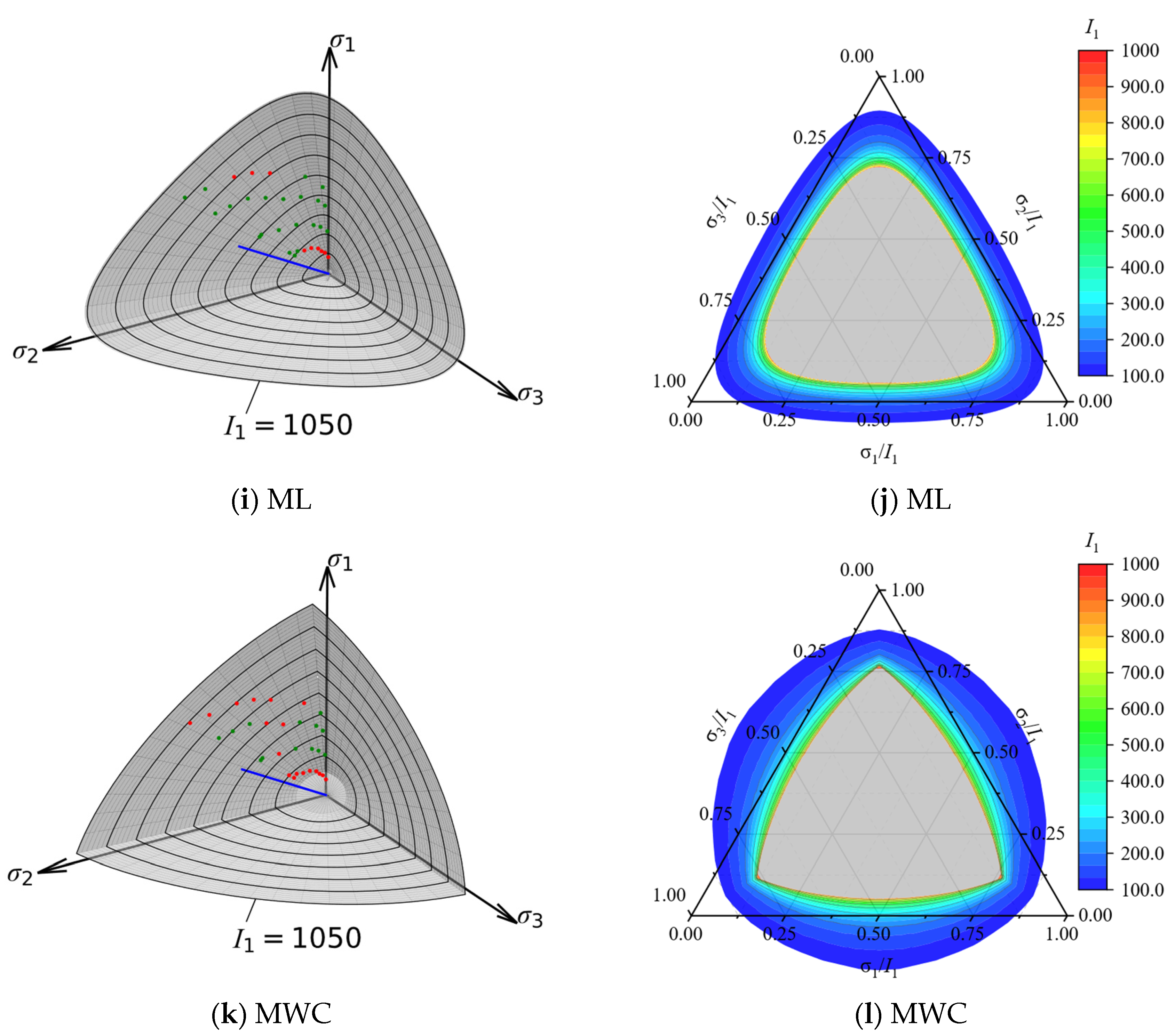
3.5. ML Criterion
3.6. MWC Criterion
4. Data Description
5. Model Building and Training
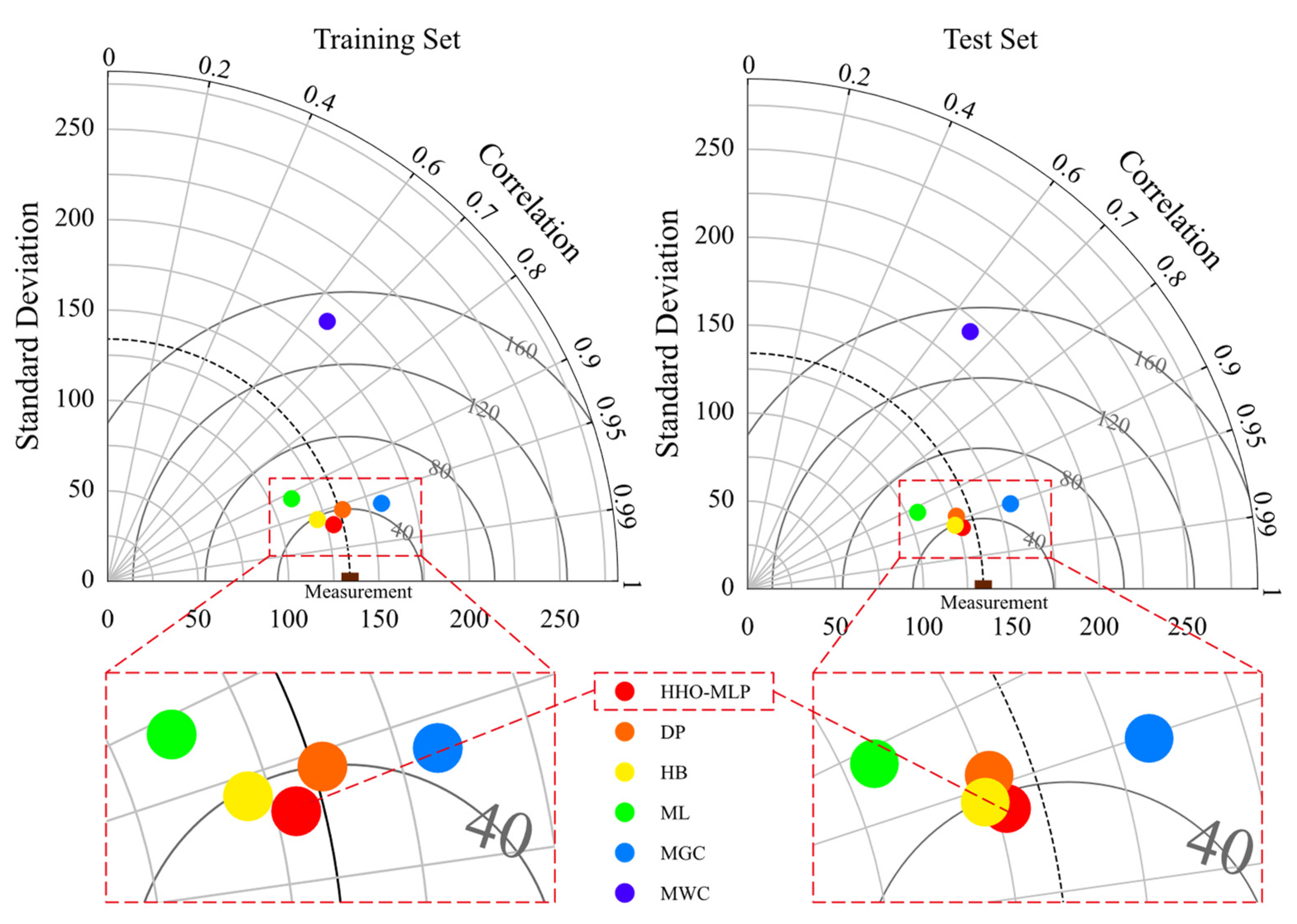
6. Performance Comparison
6.1. Comparisons Using the Collection Dataset
6.2. Comparison on the Meridian Plane
6.3. Comparison on the Deviatoric Plane
6.4. Comparison on 3D Failure Envelope
7. Conclusions
Author Contributions
Funding
Institutional Review Board Statement
Informed Consent Statement
Data Availability Statement
Conflicts of Interest
References
- Haimson, B. True triaxial stresses and the brittle fracture of rock. Pure Appl. Geophys. 2006, 163, 1101–1130. [Google Scholar] [CrossRef]
- You, M. True-triaxial strength criteria for rock. Int. J. Rock Mech. Min. Sci. 2009, 46, 115–127. [Google Scholar] [CrossRef]
- Zhou, H.; Liu, Z.; Liu, F.; Shao, J.; Li, G. Anisotropic strength, deformation and failure of gneiss granite under high stress and temperature coupled true triaxial compression. J. Rock Mech. Geotech. Eng. 2023, 16, 860–876. [Google Scholar] [CrossRef]
- Winkler, M.B.; Frühwirt, T.; Marcher, T. Elastic Behavior of Transversely Isotropic Cylindrical Rock Samples under Uniaxial Compression Considering Ideal and Frictional Boundary Conditions. Appl. Sci. 2023, 14, 17. [Google Scholar] [CrossRef]
- Vasyliev, L.; Malich, M.G.; Vasyliev, D.; Katan, V.; Rizo, Z. Improving a technique to calculate strength of cylindrical rock samples in terms of uniaxial compression. Min. Miner. Depos. 2023, 17, 43–50. [Google Scholar] [CrossRef]
- Jiang, H.; Xie, Y. A note on the Mohr–Coulomb and Drucker–Prager strength criteria. Mech. Res. Commun. 2011, 38, 309–314. [Google Scholar] [CrossRef]
- Hoek, E.; Brown, E.T. Empirical strength criterion for rock masses. J. Geotech. Eng. Div. 1980, 106, 1013–1035. [Google Scholar] [CrossRef]
- Bieniawski, Z.T. Estimating the strength of rock materials. J. S. Afr. Inst. Min. Metall. 1974, 74, 312–320. [Google Scholar] [CrossRef]
- Mogi, K. Fracture and flow of rocks under high triaxial compression. J. Geophys. Res. 1971, 76, 1255–1269. [Google Scholar] [CrossRef]
- Chang, C.; Haimson, B. True triaxial strength and deformability of the German Continental Deep Drilling Program (KTB) deep hole amphibolite. J. Geophys. Res. Solid Earth 2000, 105, 18999–19013. [Google Scholar] [CrossRef]
- Wu, S.; Zhang, S.; Zhang, G. Three-dimensional strength estimation of intact rocks using a modified Hoek-Brown criterion based on a new deviatoric function. Int. J. Rock Mech. Min. Sci. 2018, 107, 181–190. [Google Scholar] [CrossRef]
- Schwartzkopff, A.K.; Sainoki, A.; Bruning, T.; Karakus, M. A conceptual three-dimensional frictional model to predict the effect of the intermediate principal stress based on the Mohr-Coulomb and Hoek-Brown failure criteria. Int. J. Rock Mech. Min. Sci. 2023, 172, 105605. [Google Scholar] [CrossRef]
- Da Silva, M.V.; Antão, A. A new Hoek-Brown-Matsuoka-Nakai failure criterion for rocks. Int. J. Rock Mech. Min. Sci. 2023, 172, 105602. [Google Scholar] [CrossRef]
- Drucker, D.C.; Prager, W. Soil mechanics and plastic analysis or limit design. Q. Appl. Math. 1952, 10, 157–165. [Google Scholar] [CrossRef]
- Mogi, K. Effect of the intermediate principal stress on rock failure. J. Geophys. Res. 1967, 72, 5117–5131. [Google Scholar] [CrossRef]
- Lade, P.V.; Duncan, J.M. Elastoplastic stress-strain theory for cohesionless soil. J. Geotech. Eng. Div. 1975, 101, 1037–1053. [Google Scholar] [CrossRef]
- Zhou, S. A program to model the initial shape and extent of borehole breakout. Comput. Geosci. 1994, 20, 1143–1160. [Google Scholar] [CrossRef]
- Ewy, R.T. Wellbore-stability predictions by use of a modified Lade criterion. SPE Drill. Complet. 1999, 14, 85–91. [Google Scholar] [CrossRef]
- Zhang, L.; Zhu, H. Three-dimensional Hoek-Brown strength criterion for rocks. J. Geotech. Geoenviron. Eng. 2007, 133, 1128–1135. [Google Scholar] [CrossRef]
- Zhang, Q.; Shuilin, W.; Xiurun, G.; Hongying, W. Modified Mohr-Coulomb strength criterion considering rock mass intrinsic material strength factorization. Min. Sci. Technol. 2010, 20, 701–706. [Google Scholar] [CrossRef]
- Singh, M.; Raj, A.; Singh, B. Modified Mohr–Coulomb criterion for non-linear triaxial and polyaxial strength of intact rocks. Int. J. Rock Mech. Min. Sci. 2011, 48, 546–555. [Google Scholar] [CrossRef]
- Zhang, R.; Zhou, J.; Tao, M.; Li, C.; Li, P.; Liu, T. Borehole Breakout Prediction Based on Multi-Output Machine Learning Models Using the Walrus Optimization Algorithm. Appl. Sci. 2024, 14, 6164. [Google Scholar] [CrossRef]
- Fathipour-Azar, H. Polyaxial Rock Failure Criteria: Insights from Explainable and Interpretable Data-Driven Models. Rock Mech. Rock Eng. 2022, 55, 2071–2089. [Google Scholar] [CrossRef]
- Yu, B.; Zhang, D.; Xu, B.; Liu, Y.; Zhao, H.; Wang, C. Modeling of true triaxial strength of rocks based on optimized genetic programming. Appl. Soft Comput. 2022, 129, 109601. [Google Scholar] [CrossRef]
- Zhou, J.; Zhang, R.; Qiu, Y.; Khandelwal, M. A true triaxial strength criterion for rocks by gene expression programming. J. Rock Mech. Geotech. Eng. 2023, 15, 2508–2520. [Google Scholar] [CrossRef]
- Rafiai, H.; Jafari, A.; Mahmoudi, A. Application of ANN-based failure criteria to rocks under polyaxial stress conditions. Int. J. Rock Mech. Min. Sci. 2013, 59, 42–49. [Google Scholar] [CrossRef]
- Rukhaiyar, S.; Samadhiya, N.K. A polyaxial strength model for intact sandstone based on Artificial Neural Network. Int. J. Rock Mech. Min. Sci. 2017, 95, 26–47. [Google Scholar] [CrossRef]
- Rafiai, H.; Jafari, A. Artificial neural networks as a basis for new generation of rock failure criteria. Int. J. Rock Mech. Min. Sci. 2011, 48, 1153–1159. [Google Scholar] [CrossRef]
- Hong, H. Assessing landslide susceptibility based on hybrid multilayer perceptron with ensemble learning. Bull. Eng. Geol. Environ. 2023, 82, 382. [Google Scholar] [CrossRef]
- Ding, K.; Fan, S.; Dong, S. Multilayer-perceptron-based prediction of sand-over-clay bearing capacity during spudcan penetration. Int. J. Nav. Archit. Ocean Eng. 2022, 14, 100479. [Google Scholar] [CrossRef]
- Vinay, L.S.; Bhattacharjee, R.M.; Ghosh, N.; Kumar, S. Machine learning approach for the prediction of mining-induced stress in underground mines to mitigate ground control disasters and accidents. Geomech. Geophys. Geo-Energy Geo-Resour. 2023, 9, 159. [Google Scholar] [CrossRef]
- Almeida, L.B. Multilayer perceptrons. In Handbook of Neural Computation; CRC Press: Boca Raton, FL, USA, 2020; pp. C1. 2: 1–C1. 2: 30. [Google Scholar]
- Xu, Y.; Li, F.; Asgari, A. Prediction and optimization of heating and cooling loads in a residential building based on multi-layer perceptron neural network and different optimization algorithms. Energy 2022, 240, 122692. [Google Scholar] [CrossRef]
- Heidari, A.A.; Mirjalili, S.; Faris, H.; Aljarah, I.; Mafarja, M.; Chen, H. Harris hawks optimization: Algorithm and applications. Future Gener. Comput. Syst. 2019, 97, 849–872. [Google Scholar] [CrossRef]
- Yang, X.-S. Nature-Inspired Metaheuristic Algorithms; Luniver Press: Bristol, UK, 2010. [Google Scholar]
- Hill, R. The Mathematical Theory of Plasticity; Oxford University Press: Oxford, UK, 1998; Volume 11. [Google Scholar]
- Marinos, P.; Hoek, E. Estimating the geotechnical properties of heterogeneous rock masses such as flysch. Bull. Eng. Geol. Environ. 2001, 60, 85–92. [Google Scholar] [CrossRef]
- Feng, F.; Li, X.; Du, K.; Li, D.; Rostami, J.; Wang, S. Comprehensive evaluation of strength criteria for granite, marble, and sandstone based on polyaxial experimental tests. Int. J. Geomech. 2020, 20, 04019155. [Google Scholar] [CrossRef]
- Kwasniewski, M.; Takahashi, M.; Li, X. Volume changes in sandstone under true triaxial compression conditions. In Proceedings of the 10th ISRM Congress, Sandton, South Africa, 8–12 September 2003. [Google Scholar]
- Pobwandee, T. Effects of Intermediate Principal Stress on Compressive Strength and Elasticity of Phra Wihan Sandstone. Master’s Thesis, School of Geotechnology, Institute of Engineering, Suranaree University of Technology, Nakhon Ratchasima, Thailand, 2010. [Google Scholar]
- Rukhaiyar, S.; Samadhiya, N.K. Strength behaviour of sandstone subjected to polyaxial state of stress. Int. J. Min. Sci. Technol. 2017, 27, 889–897. [Google Scholar] [CrossRef]
- Takahashi, M.; Koide, H. Effect of the intermediate principal stress on strength and deformation behavior of sedimentary rocks at the depth shallower than 2000 m. In Proceedings of the ISRM International Symposium, Pau, France, 30 August–2 September 1989; p. ISRM–IS-1989-1003. [Google Scholar]
- Walsri, C.; Poonprakon, P.; Thosuwan, R.; Fuenkajorn, K. Compressive and tensile strengths of sandstones under true triaxial stresses. In Proceedings of the 2nd Thailand Symposium on Rock Mechanics, Chonburi, Thailand, 12–13 March 2009; pp. 199–218. [Google Scholar]
- Feng, X.-T.; Kong, R.; Zhang, X.; Yang, C. Experimental study of failure differences in hard rock under true triaxial compression. Rock Mech. Rock Eng. 2019, 52, 2109–2122. [Google Scholar] [CrossRef]
- Gao, Y.-H.; Feng, X.-T.; Zhang, X.-W.; Feng, G.-L.; Jiang, Q.; Qiu, S.-L. Characteristic stress levels and brittle fracturing of hard rocks subjected to true triaxial compression with low minimum principal stress. Rock Mech. Rock Eng. 2018, 51, 3681–3697. [Google Scholar] [CrossRef]
- Smart, B.; Somerville, J.; Crawford, B.R. A rock test cell with true triaxial capability. Geotech. Geol. Eng. 1999, 17, 157–176. [Google Scholar] [CrossRef]
- He, P.-F.; Ma, X.-D.; He, M.-C.; Tao, Z.-G.; Liu, D.-Q. Comparative study of nine intact rock failure criteria via analytical geometry. Rock Mech. Rock Eng. 2022, 55, 3083–3106. [Google Scholar] [CrossRef]
- Murlidhar, B.R.; Nguyen, H.; Rostami, J.; Bui, X.; Armaghani, D.J.; Ragam, P.; Mohamad, E.T. Prediction of flyrock distance induced by mine blasting using a novel Harris Hawks optimization-based multi-layer perceptron neural network. J. Rock Mech. Geotech. Eng. 2021, 13, 1413–1427. [Google Scholar] [CrossRef]
- Huang, S.; Zhou, J. An enhanced stability evaluation system for entry-type excavations: Utilizing a hybrid bagging-SVM model, GP and kriging techniques. J. Rock Mech. Geotech. Eng. 2024; in press. [Google Scholar] [CrossRef]
- Zhou, J.; Yang, P.; Peng, P.; Khandelwal, M.; Qiu, Y. Performance evaluation of rockburst prediction based on PSO-SVM, HHO-SVM, and MFO-SVM hybrid models. Min. Metall. Explor. 2023, 40, 617–635. [Google Scholar] [CrossRef]
- Qiu, Y.; Zhou, J.; He, B.; Armaghani, D.J.; Huang, S.; He, X. Evaluation and interpretation of blasting-induced tunnel overbreak: Using heuristic-based ensemble learning and gene ex-pression programming techniques. Rock Mech. Rock Eng. 2024, 1–29. [Google Scholar] [CrossRef]
- Zhou, J.; Qiu, Y.; Armaghani, D.J.; Zhang, W.; Li, C.; Zhu, S.; Tarinejad, R. Predicting TBM penetration rate in hard rock condition: A comparative study among six XGB-based metaheuristic techniques. Geosci. Front. 2021, 12, 101091. [Google Scholar] [CrossRef]
- Zhang, Y.L.; Qiu, Y.G.; Armaghani, D.J.; Monjezi, M.; Zhou, J. Enhancing rock fragmentation prediction in mining operations: A Hybrid GWO-RF model with SHAP interpretability. J. Cent. South Univ. 2024, 1–14. [Google Scholar] [CrossRef]
- Zhou, J.; Qiu, Y.; Zhu, S.; Armaghani, D.J.; Li, C.; Nguyen, H.; Yagiz, S. Optimization of support vector machine through the use of metaheuristic algorithms in forecasting TBM advance rate. Eng. Appl. Artif. Intell. 2021, 97, 104015. [Google Scholar] [CrossRef]
- Taylor, K.E. Summarizing multiple aspects of model performance in a single diagram. J. Geophys. Res. Atmos. 2001, 106, 7183–7192. [Google Scholar] [CrossRef]
- Krabbenhoft, K.; Lyamin, A. Generalised Tresca criterion for undrained total stress analysis. Géotech. Lett. 2015, 5, 313–317. [Google Scholar] [CrossRef]


| Number | Number of Data | (MPa) | (MPa) | (MPa) | References | |||
|---|---|---|---|---|---|---|---|---|
| Min | Max | Min | Max | Min | Max | |||
| 1 | 29 | 92.1 | 492.1 | 10 | 413 | 10 | 100 | [38] |
| 2 | 17 | 87.48 | 302.8 | 0 | 62.5 | 0 | 37.5 | [39] |
| 3 | 23 | 25.91 | 172 | 0 | 60 | 0 | 20 | [40] |
| 4 | 24 | 34.62 | 128.68 | 0 | 24 | 0 | 10 | [41] |
| 5 | 44 | 74.22 | 279 | 0 | 171 | 0 | 50 | [42] |
| 6 | 20 | 75.4 | 194 | 0 | 118.3 | 0 | 15 | [42] |
| 7 | 14 | 48.5 | 159.1 | 0 | 24 | 0 | 6.6 | [43] |
| 8 | 14 | 49.4 | 165.9 | 0 | 24 | 0 | 6.6 | [43] |
| 9 | 14 | 46.4 | 147.6 | 0 | 24 | 0 | 6.6 | [43] |
| 10 | 31 | 60 | 465 | 0 | 436 | 0 | 50 | [44] |
| 11 | 27 | 184.17 | 378.68 | 0 | 160 | 0 | 10 | [45] |
| 12 | 20 | 23.69 | 192.97 | 0 | 55.2 | 0 | 55.2 | [46] |
| 13 | 78 | 56.1 | 648 | 0 | 620.7 | 0 | 150 | [47] |
| 14 | 62 | 29.7 | 370.2 | 0 | 346.3 | 0 | 150 | [47] |
| Name | Equation |
|---|---|
| sigmoid | |
| softplus | |
| swish | |
| tanh |
| Sandstone Number | DP | HB | MGC | ML | MWC | |||
|---|---|---|---|---|---|---|---|---|
(MPa) | ||||||||
| 1 | 0.17 | 33.87 | 21 | 3.9 | 21.3 | 13.71 | 2.84 | 7.6 |
| 2 | 0.33 | 25.04 | 21 | 5.87 | 17.38 | 45.7 | 4.77 | 1.37 |
| 3 | 0.32 | 13.73 | 21 | 8.96 | 12.16 | 54.21 | 0.64 | 0.73 |
| 4 | 0.37 | 7.25 | 21 | 7.13 | 10.29 | 60.11 | 6.19 | 1255.77 |
| 5 | 0.21 | 28.3 | 13.86 | 3.62 | 19.29 | 17.18 | 3.09 | 0.14 |
| 6 | 0.16 | 38.4 | 18.68 | 4.19 | 20 | 18.93 | 3.89 | 0.26 |
| 7 | 0.46 | 1.78 | 21 | 12.04 | 6.67 | 184.7 | 9.29 | 0.63 |
| 8 | 0.45 | 6.27 | 21 | 14.07 | 8.31 | 169.15 | 10.65 | 4.91 |
| 9 | 0.43 | 4.58 | 21 | 10.56 | 7.86 | 138.2 | 8.28 | 0.89 |
| 10 | 0.23 | 31.92 | 21 | 6.02 | 17.54 | 37 | 4.41 | 2.23 |
| 11 | 0.18 | 92.66 | 21 | 6.56 | 33.79 | 31.26 | 6.21 | 0.66 |
| 12 | 0.24 | 9.72 | 15.01 | 3.49 | 13.54 | 16.12 | 0.43 | 0.97 |
| 13 | 0.17 | 53.62 | 21 | 3.8 | 29.63 | 11.44 | 1.04 | 1.87 |
| 14 | 0.1 | 43.29 | 13 | 2.43 | 26.56 | 1.68 | 0.73 | 3.6 |
| Model | Training | Test | ||||||
|---|---|---|---|---|---|---|---|---|
| R2 | MAE | RMSE | MAPE | R2 | MAE | RMSE | MAPE | |
| HHO-MLP | 0.9700 | 25.4266 | 32.7273 | 0.1435 | 0.9615 | 28.5801 | 36.9180 | 0.1587 |
| DP | 0.9564 | 28.6053 | 39.9217 | 0.1681 | 0.9444 | 31.3053 | 44.2664 | 0.2138 |
| HB | 0.9594 | 39.2814 | 51.345 | 0.1819 | 0.9562 | 42.8719 | 54.2242 | 0.2011 |
| MGC | 0.9618 | 32.105 | 46.4841 | 0.1382 | 0.9514 | 32.6736 | 50.8198 | 0.14 |
| ML | 0.9124 | 54.2102 | 71.7347 | 0.2601 | 0.9119 | 53.1789 | 71.7476 | 0.237 |
| MWC | 0.6453 | 80.4979 | 148.0962 | 0.4868 | 0.6543 | 83.0136 | 149.1945 | 0.4666 |
Disclaimer/Publisher’s Note: The statements, opinions and data contained in all publications are solely those of the individual author(s) and contributor(s) and not of MDPI and/or the editor(s). MDPI and/or the editor(s) disclaim responsibility for any injury to people or property resulting from any ideas, methods, instructions or products referred to in the content. |
© 2024 by the authors. Licensee MDPI, Basel, Switzerland. This article is an open access article distributed under the terms and conditions of the Creative Commons Attribution (CC BY) license (https://creativecommons.org/licenses/by/4.0/).
Share and Cite
Zhang, R.; Zhou, J.; Wang, Z. Innovative Data-Driven Machine Learning Approaches for Predicting Sandstone True Triaxial Strength. Appl. Sci. 2024, 14, 7855. https://doi.org/10.3390/app14177855
Zhang R, Zhou J, Wang Z. Innovative Data-Driven Machine Learning Approaches for Predicting Sandstone True Triaxial Strength. Applied Sciences. 2024; 14(17):7855. https://doi.org/10.3390/app14177855
Chicago/Turabian StyleZhang, Rui, Jian Zhou, and Zhenyu Wang. 2024. "Innovative Data-Driven Machine Learning Approaches for Predicting Sandstone True Triaxial Strength" Applied Sciences 14, no. 17: 7855. https://doi.org/10.3390/app14177855