Abstract
In this study, we aimed to assess the capacity of a physics-based earthquake simulator to improve our understanding of the seismogenic process. In this respect, we applied a previously tested earthquake simulator to two well-known and completely different seismogenic fault systems, namely the Italian Apennines and the Nankai subduction in Japan, for which long historical records of strong earthquakes are available. They are characterized by different fault mechanisms, fault sizes, and slip rates. Because of the difference in slip rates, the time scale of the seismicity patterns is different for the two systems (several hundreds of years for the Apennines and a few tens of years for the Nankai Fault). The results of simulations that produced synthetic catalogues of 100,000 years show these significant long-term seismicity patterns characterizing the seismic cycles for both seismogenic areas as follows: The average stress and the occurrence rate of earthquakes increase in the long term as the next major earthquake approaches; while the average stress increases uniformly, the occurrence rate stops increasing well in advance of the mainshocks; the b-value exhibits a long-term increase before major earthquakes and a fast decrease shortly before the mainshocks. Even if no specific statistical tool was applied for the quantification of the similarities between the seismicity patterns of the two seismic areas, such similarities are clearly justified by the large number of seismic cycles included in the 100,000-year synthetic catalogues. The paper includes a discussion on the capability of the simulation algorithm to reliably represent the real long-term seismogenic process. This question is difficult to answer because the available historical observations are of too short a duration to provide significant statistical results. In spite of the limitations characterizing the use of earthquake simulators for time-dependent earthquake hazard assessment, and the lack of convincing mechanistic explanations of the specific seismic patterns reproduced by our simulator algorithm, our results encourage further investigations into the application of simulators for the development of seismogenic models, including short-term features.
1. Introduction
Since the groundbreaking research by Rundle and Jackson (1977) [1], followed by Rundle and Brown (1991) [2] and Ward (1992) [3], physics-based earthquake simulators have increasingly captivated the seismological community as a valuable tool for formulating and validating hypotheses about the earthquake process and interpreting earthquake data. These simulators can reproduce essential statistical relationships such as magnitude–frequency distributions, temporal patterns like the Omori law, and characteristics of earthquake clustering. By overcoming the inherent limitations of real-world observations such as completeness, homogeneity, and duration, earthquake simulators facilitate the assessment of diverse seismogenic process models and utilizing renewal models. Contributions from Ward (1996 [4], 2000 [5], and 2012 [6]), Tullis (2012) [7], as well as Wilson et al. (2017) [8] and Shaw et al. (2018) [9], have further shown the capacity of their respective algorithms.
While acknowledging that even the most sophisticated earthquake simulators are simplified models of the intricate reality of the earthquake process and that not all findings derived from such models can be exhaustively validated against real earthquakes, there is a consensus on their efficacy in enhancing the overall testing protocols for earthquake forecasting. This sentiment is shared by experts such as Schultz et al. (2015) [10], Christophersen et al. (2017) [11], Field (2015 [12], 2019 [13]), and Rundle et al. (2022) [14].
We are interested in testing the capacity of the physics-based earthquake simulator developed in the last decade inside our research team (Console et al., 2022 [15], and references therein) to improve our comprehension of the seismogenic process. With this aim, we applied a previously tested version of the earthquake simulator to two well-known and completely different seismogenic structures, namely the Northern and Central Apennines, Italy, fault systems (since now referred to as CNAFS), and the Nankai megathrust, Japan, fault system (since now referred to as NMTFS).
The earthquake simulation algorithm applied in our study is mainly based on simple physical principles underlying the elastic-rebound theory introduced by Reid (1910) [16], and the theory of the elasticity for the computation of the Coulomb stress transfer from a ruptured fault patch to any other surrounding potential source (Catalli 2007 [17]). No use is made of non-linear physical ingredients such as the Dieterich Rate and State model or viscosity and fluid flow effects, based on the Occam principle that “the simpler the better”, as shown by the realistic seismic patterns produced by our model.
The simulator algorithm assumes a constant stress drop at each rupture of single patches and includes a set of (mainly two) free parameters that can be subjectively chosen by the user to control a rupture growth and better represent the real observations in a suitable way. In particular, Console and Carluccio (2020) [18] gave detailed examples of the way these parameters affect the magnitude distribution of the synthetic catalogues and how the “characteristic earthquake” effect enhances the production of events rupturing a substantial fraction of entire fault sources rather than the background seismicity, which follows the Gutenberg–Richter law more closely. In the present study, we adopted the same set of parameters as in Console et al. (2022b) [15].
As already stated, in this work, we compared the seismogenic process in the following two completely different geodynamic contexts: the main crustal sources in Central Italy with the large sources of the subduction interface in Southwestern Japan. Reliable historical earthquakes are available for the distinct 43 seismogenic fault systems straddling the Northern and Central Apennines and for the 700 km long Japanese fault system (Figure 1).
The strongest earthquake in the Italian study area occurred on 14 January 1703 (having Mw 6.9, and intensity XI MCS), and struck the Valnerina (Rovida et al., 2022 [19]; Table 1). All four strongest earthquakes for the CNAFS in the last 10 centuries occurred after 1700 A.D. (Table 1), and none of these four earthquakes are known as having fully ruptured the whole seismogenic fault system to which they are assigned in Table 1.
The NMTFS generated several earthquakes of a magnitude larger than 8.0 in the last 10 centuries; therefore, these earthquakes have occurred repeatedly at intervals of 100 to 150 years along the Nankai Trough (e.g., Parsons et al., 2012 [20]; Yamamoto et al., 2022 [21]; Table 1).
Through the definition of the moment magnitude (Hanks and Kanamori 1979 [22]), we estimated the seismic moments released by the historical earthquakes reported in Table 1 since the year 1000 for the CNAFS and the NMTFS, obtaining 5.23 1019 Nm and 4.60 1022 Nm, respectively.
In Italy, the causative sources of the main earthquakes of the study area are as follows: (1) the NW–SE-trending post-orogenic normal faults in the axial portion of the Apennines (e.g., Vannoli et al., 2012 [23]), (2) the NE-verging syn-orogenic thrusts towards the Adriatic foreland (e.g., Vannoli et al., 2015 [24]), and (3) the ENE–WSW-trending strike-slip faults bounding the Central Apennines thrust fronts to the South (DISS Working Group 2021 [25]). Most of the earthquakes of the CNAFS occurred between 1 and 15 km depth, above the basal detachment of the thrust fronts. The active extension is accommodated by normal faulting, which dominates along the hinge of the chain (e.g., Di Bucci et al., 2011 [26]).
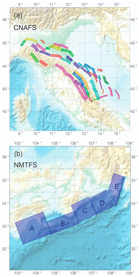
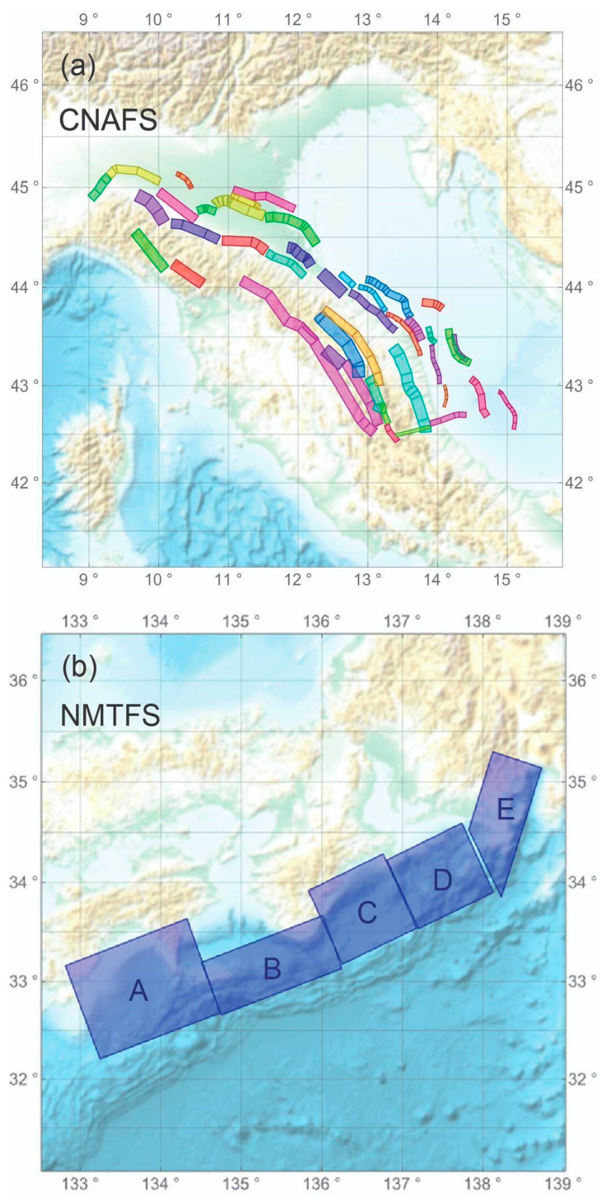

Figure 1.
(a) A total of 43 seismogenic randomly colored fault systems—divided into 198 trapezoidal segments—straddling the northern and central Apennines (DISS Working Group 2021 [25]); (b) the Japanese megathrust fault system is divided into 5 fault segments (Parsons et al., 2012 [20]). Geometric and kinematics parameters of the seismogenic sources adopted in the simulator algorithm are shown in Tables S1 and S2 of the Supplementary Material.
Table 1.
Historical and instrumental earthquakes that ruptured segments from the year 1000 of the CNAFS (having a magnitude equal to or larger than 6.5; DISS Working Group 2021 [25]; Rovida et al., 2022 [19]; Table S1), and the NMTFS (having a magnitude equal to or larger than 7.9; Parsons et al., 2012 [20] and references therein; Table S2). For CNAFS, magnitudes refer to Mw (converted from macroseismic data for historical earthquakes or measured for the 2016 event). For NMTFS, magnitudes were mostly obtained from tsunami records and possibly referable to Mw.
| ID | Date | M | Causative Source(s) |
|---|---|---|---|
| 1_CNAFS | 14 January 1703 | 6.9 | The southern half of the ITCS028 |
| 2_CNAFS | 3 June 1781 | 6.5 | The northern 30% of the ITCS129 |
| 3_CNAFS | 7 September1920 | 6.5 | The northern half of the ITCS083 |
| 4_CNAFS | 30 October 2016 | 6.6 | The southern half of the ITCS127 |
| 1_NMTFS | 17 December 1096 | 8.4 | CD/CDE |
| 2_NMTFS | 22 February 1099 | 8.4 | AB |
| 3_NMTFS | 3 August 1361 | 8.4 | AB/ABCD/ABCDE |
| 4_NMTFS | 20 September 1498 | 8.6 | CDE/ABCDE |
| 5_NMTFS | 3 February 1605 | 7.9 | ABCD |
| 6_NMTFS | 28 October 1707 | 8.4 | ABCDE |
| 7_NMTFS | 23 December 1854 | 8.4 | CDE |
| 8_NMTFS | 24 December 1854 | 8.4 | AB |
| 9_NMTFS | 7 December 1944 | 8.2 | CD |
| 10_NMTFS | 20 December 1946 | 8.2 | AB |
In Japan, the interface megathrust earthquakes occur between the overriding Eurasian/Amur continental plate and the subducting Philippine Sea oceanic plate.
The seismogenic model of NMTFS is subdivided into five main 100–150 km long fault segments along the trough axis and almost corresponds to the distribution of forearc basins (e.g., Fujiwara et al., 2023 [27], and references therein). The seismogenic model of CNAFS includes 43 onshore and offshore seismogenic sources characterized by extensional and compressive kinematics (DISS Working Group 2021 [25]).
Different fault mechanisms, fault sizes, and slip rates characterize the seismogenic sources of the two regions. Table 2 summarizes their main characteristics, while Tables S1 and S2 in the Supplementary Materials list the geometrical and kinematics parameters of the seismogenic sources adopted in the simulator algorithm of the CNAFS and the NMTFS, respectively (see Console et al., 2022b [15] and references therein).
Table 2.
Summary of the main characteristics of the two geodynamic contexts.
Notice that very different slip rates characterize the segments of the Japanese and Italian fault systems, and both systems can rupture separately or simultaneously with each other.
2. Comparison of Long-Term Features
In this application of the simulation algorithm, which does not contain any distinction among the different fault mechanisms, except for the stress interaction among different sources, we adopted the same set of free parameters used by Console et al. (2022b) [15] for both study areas. Applying the same set of parameters to these two geologically distinct regions (CNAFS and NMTFS) might appear inappropriate due to the inherent differences in their tectonic settings. In fact, finding a justification for our choice based on the information provided by the historical records reported in Table 1 is a difficult task, especially for CNAFS. Console et al., 2022b [15] tried a set of nine combinations of free parameters and found the combination of the two parameters adopted in their study as the most appropriate for simulating the clustering properties of the observed seismicity. Nevertheless, the characteristic earthquake features of the synthetic catalogue were not recognizable in the observed seismicity, most likely due to the short duration of the historical catalogue (370 years in their study) in comparison with the expected recurrence time of the characteristic earthquake of the CNAFS of some thousands of years. For short-term clustering, Figure 8 of Console et al., 2022b [15] found that the simulator could reproduce reliable features of foreshocks–aftershocks sequences and b-value variations.
We produced for CNAFS a synthetic catalog lasting 100,000 years and containing more than 300,000 Mw ≥ 4.2 events, while for NMTFS, a catalogue lasting 100,000 years and containing more than 1,000,000 Mw ≥ 5.0 events was obtained. The largest magnitudes reported in the two simulated catalogues are 7.55 (CNAFS) and 8.66 (NMTFS). For NMTFS, the largest magnitude is similar to the one reported in Table 1 and may be related to the rupture of the whole fault system in a single event, while for the more complex CNAFS, there is a difference in the order of a half magnitude unit between the largest simulated and observed magnitudes, referable to the shortness of the historical catalogue as outlined in the previous paragraph.
A comparison between the occurrence rates of the two study areas was performed by computing the average inter-event times for earthquakes of Mw ≥ 7.0 within a distance of 100 km from each other. This computation sorted out a value of 1920 and 42 years for CNAFS and NMTFS, respectively. Similarly, we computed the seismic moments released by CNAFS and NMTFS, obtaining 5.15 1017 Nm/year and 8.12 1019 Nm/year, respectively. These values are, respectively, equivalent to the seismic moment released by a yearly earthquake of magnitudes 5.74 and 7.11. Both comparisons clearly show the great disparity of seismic activity between the two fault systems, due to the large difference between both the fault sizes and the slip rate of the two seismogenic models. In our simulation algorithm, the rate of seismic moment released by the fault systems is controlled uniquely by the dimensions of the sources and their slip rates (as the shear modulus G of the elastic medium is assigned as a constant) and not by the free parameters used for controlling the rupture growths.
The values of the seismic moments previously obtained for the historical earthquakes of Table 1 are smaller than those resulting from the simulations for the same period of 1024 years for both seismogenic systems considered in this study. For the CNAFS in particular, the seismic moment released by the four strongest historical earthquakes is an order of magnitude smaller than that which was computed through the seismogenic model of the simulator application. This discrepancy can be justified by a series of factors, among which are the following: overestimation of the slip rate adopted in the seismogenic model (for the CNAFS, it was obtained by the average of a range of values reported by the DISS database); missing the fraction of seismic moment released by earthquakes having a magnitude smaller than 6.5; uncertainty in the magnitude estimate of old earthquakes; lack of large magnitude earthquakes during the first seven centuries over a total period of ten centuries. The same kind of test carried out on the NMTFS exhibits a much better agreement between the synthetic and observed seismic moment, with a difference of the order of 40%, partly justifiable by the omission of events having a magnitude smaller than 7.9. Our results for the NMTFS can be compared with Meade (2023) [28], who used a 3D model of the Nankai fault system to simulate a 1250-year earthquake sequence, including over 700 Mw 5.5–8.5 events and periods of quiescence followed by aftershocks. Despite differences in the methodology, such as Meade’s use of the G–R law versus our physics-based approach, we found remarkable similarities in the periodicity and timing of strong events in both studies.
To analyze the effect of smaller magnitude events on the total seismic moment released by the CNAFS, we have computed the seismic moment after 1000 A.D. for all the 36 earthquakes of magnitude M ≥ 6.0 reported by CPTI (Rovida et al., 2022 [19]), 14 of which occurred before 1700 A.D. In this case, we obtained a total of 1.42 1020 Nm, nearly three times larger than the value obtained for M ≥ 6.5 only.
We applied a stacking procedure for analyzing the temporal pattern of seismicity before and after earthquakes of magnitude equal to or greater than a target magnitude Mpivot (hereafter called pivot event). For each event of M ≥ Mpivot, the catalog was scanned for a time Tdur preceding and the same time Tdur following such an event, dividing these two periods in bins of Tbin length. The events that occurred in the same time bin were considered if their epicenters were within a distance Rdist from the epicenter of the target earthquake and their magnitudes exceeded a threshold Mmin. The procedure was repeated for all M ≥ Mpivot earthquakes, and all the events found in each bin were analyzed together (see Table 3).
Table 3.
Summary of the seismogenic model features and time–space ranges for the two study areas.
Our analysis concerned the following:
- The average stress computed on the cells containing the epicenters of all the earthquakes selected in every time bin at their respective origin time;
- The number of earthquakes selected in every time bin;
- The b-value of the earthquakes selected in every time bin.
2.1. Stress History
In our simulator algorithm, the stress in each cell of the fault system increases in time by tectonic loading, decreasing by a constant stress drop of 3 MPa at the instant of each rupture, and changing by co-seismic Coulomb stress transfer released by each ruptured cell. The simulator algorithm allowed us to compile a dataset with the time history of the stress values on each cell of the model, before and after every simulated earthquake. The results of the stress analysis performed by the stacking procedure mentioned above are given in Figure 2.
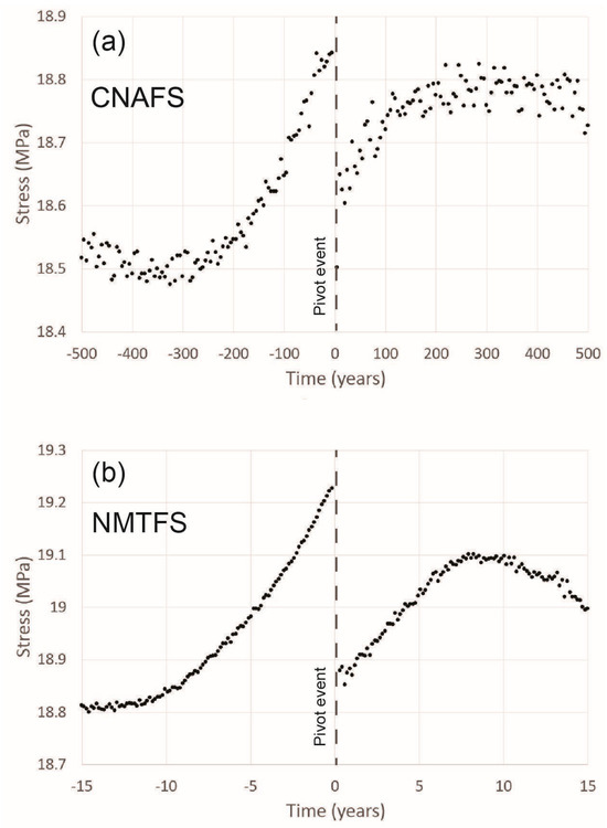
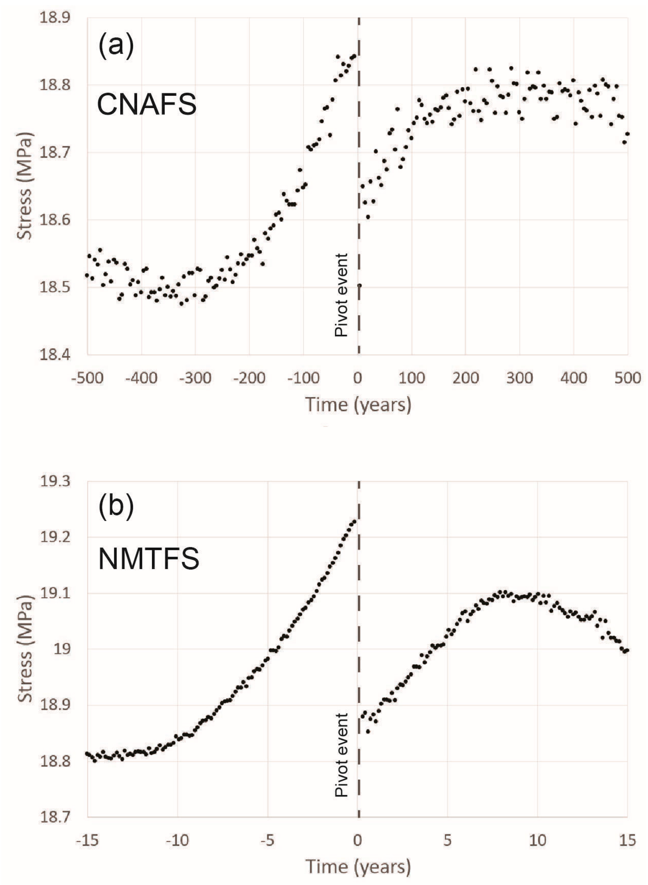
Figure 2.
(a) Average stress preceding and following any M 5.2+ earthquake, obtained from the 100,000 years simulation for the CNAFS; (b) As in the top for the M 5.8+ earthquakes in the NMTFS. The larger dispersion of points in the plot concerning the CNAFS can be ascribed to the smaller number of events available in the application of the stacking procedure.
The plots in Figure 2 have a very similar shape, taking into account a ratio of about a factor of 30 in the time scale. The more scattered behavior of the CNAFS may be ascribed to the higher heterogeneity of this fault system compared to NMTFS. Both plots exhibit a constant increase in stress until the time of the pivot event, followed by a sudden decrease at the instant of its occurrence. As expected, this feature is consistent with Reid’s (1910) [16] elastic-rebound theory, which is the basic ingredient of our simulation algorithm.
Figure 2 shows that for both the CNAFS and the NMTFS, the average stress has a trend to partially recover the values preceding the preparatory phase of pivot events, but it does not show the length of time necessary for starting the new preparatory phase of stress increase. Producing a plot of the same kind with a longer time length for both the CNAFS and the NMTFS, we found that the average stress fully recovers its standby value in about 1000 years and 50 years, respectively, after the pivot event.
2.2. Occurrence Rates
We examined the seismicity produced by the simulator in a long-term time interval before and after events of larger magnitude. The previously mentioned stacking technique was applied to the number of pairs of events of magnitude exceeding the thresholds listed in Table 3. The time difference and the largest distance between the two events of each pair are also reported in Table 3 for CNAFS and NMTFS, respectively. The results of this analysis are depicted in Figure 3.
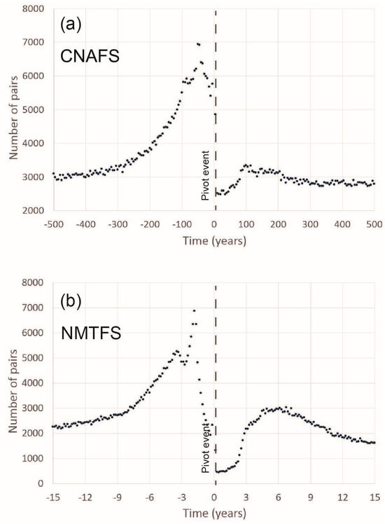
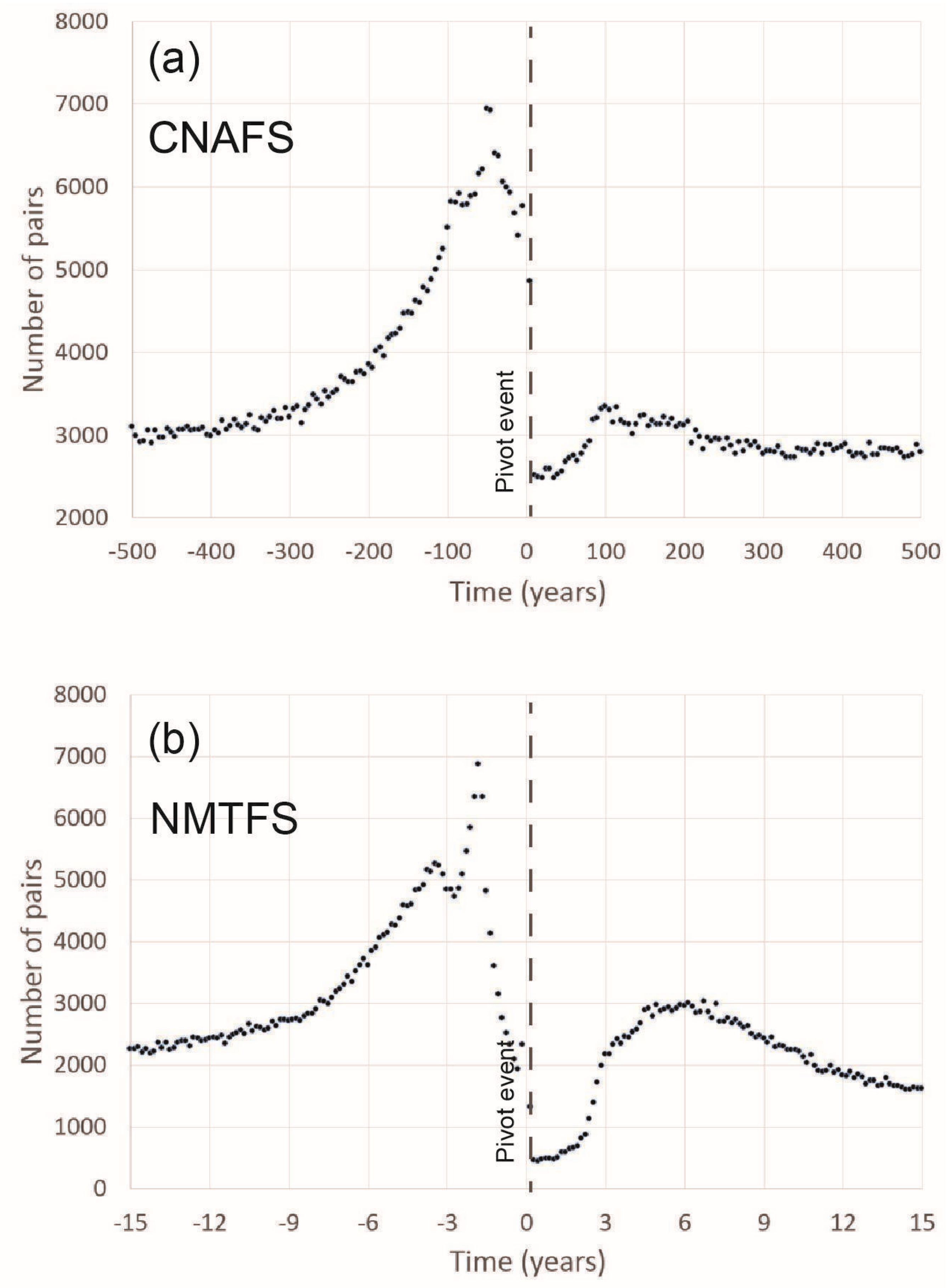
Figure 3.
(a) Stacked number of M 4.2+ earthquakes preceding and following an M 5.2+ earthquake, obtained from the 100,000 years simulation in a long-term scale for the CNAFS. The long-term plot shows acceleration before and quiescence after the strong event. (b) As in the top, for the M 5.2+ earthquakes preceding and following an M 5.8+ earthquake in the NMTFS.
Our findings, concerning the CNAFS, unveil a discernible pattern of seismic activity characterized by a notable increase several centuries preceding pivot events. Additionally, we observe some oscillations starting approximately 100 years prior to the occurrence of the pivot events, followed by a pronounced decrease in seismic activity in the last 50 years, and concluded with a final increase just in the last 5 years. For the NMTFS, a precursory pattern with two maxima of seismic activity 4 years and 2 years before the pivot event can be noted. The complexity of these patterns can be ascribed to the variable slip rate on the different segments composing both fault systems.
Regarding the seismicity rates observed in the simulations, the two completely different geodynamic contexts exhibit a sharp decrease just at the time of the pivot events, followed by a slow increase lasting about 100 years and 6 years in the CNAFS and the NMTFS, respectively (Figure 3).
2.3. b-Values Time Variations
We examined the b-value time variations of the seismicity produced by the simulator in a long-term time interval before and after pivot events. In this case, the b-value was computed as the average obtained by the stacking procedure on the earthquakes that occurred within each of the 200 bins by which the total time window is divided. The previously mentioned stacking technique was applied for the computation of b-values of sets of events falling in the time bins and magnitude exceeding the thresholds listed in Table 3. The results of this analysis are depicted in Figure 4.
Our plot, concerning the b-value on specific areas of the CNAFS, exhibits a clear increase starting about 100 years before any M 5.2+ earthquake. Additionally, a decrease is notable in the last bin lasting 5 years before the pivot events. The decrease continues after the pivot events for about 150 years until the b-value preceding the precursory increase is restored. For the NMTFS, the same pattern is observable but for pivot events of M 5.8+ and in a time scale approximately 30 times shorter.
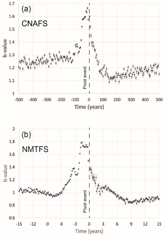
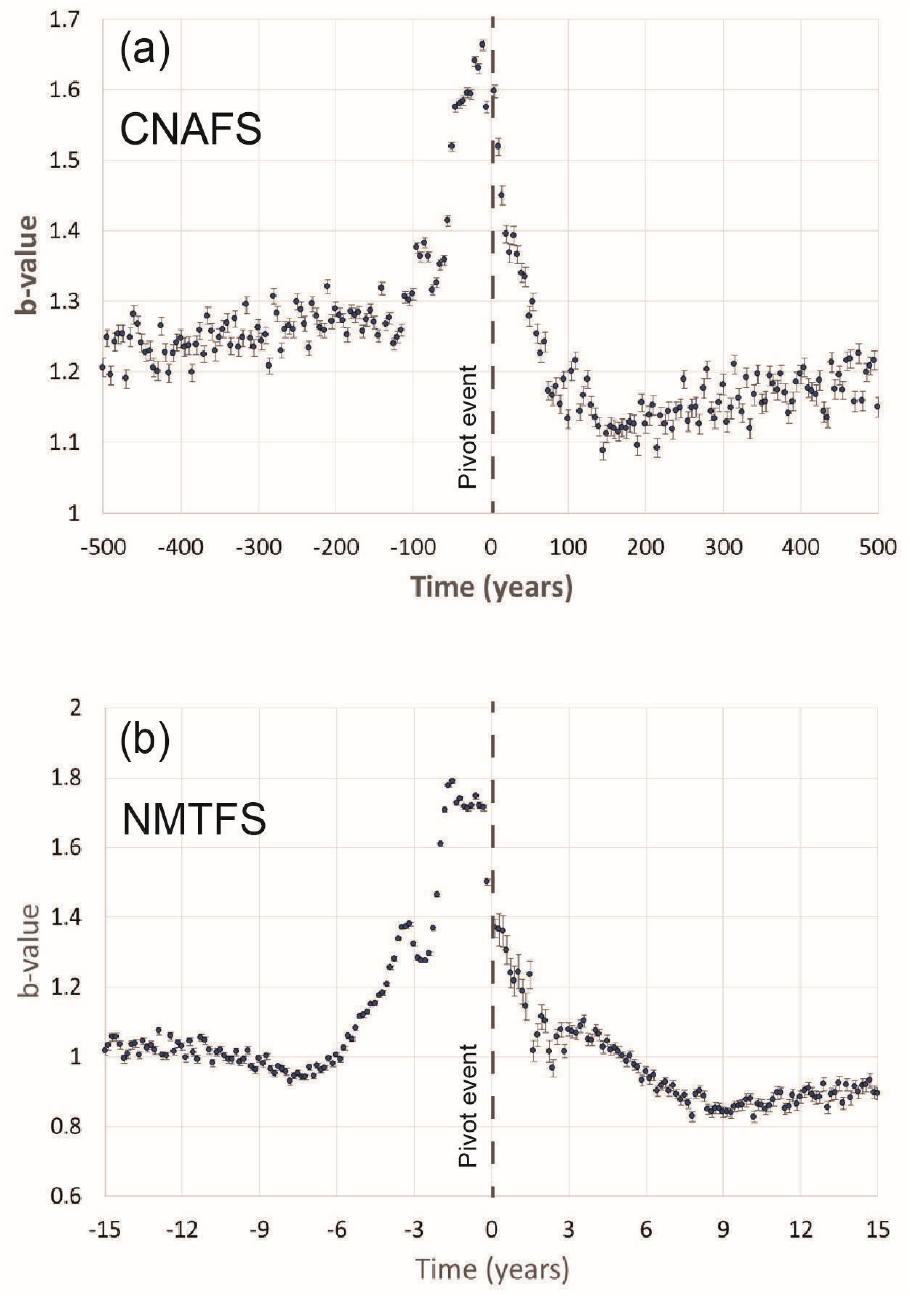
Figure 4.
(a) Average b-values with their standard deviations of M 4.2+ earthquakes preceding and following an M 5.2+ earthquake, obtained from the 100,000 years simulation in a long-term scale for the CNAFS. The long-term plot shows an increase in b-values before and a decrease after the strong event. (b) As in the top, for the M 5.2+ earthquakes preceding and following an M 5.8+ earthquake in the NMTFS. The error bars represent the standard deviation of the b-values computed using the formula proposed by Shi and Bolt (1982) [29].
3. Discussion and Conclusions
The primary objective of this research was to achieve a deeper understanding and enhance the potential predictability of seismic activities through simulations executed via an algorithm grounded in a suitable modeling approach of the sources responsible for major earthquakes. The capacity of the simulation algorithm in this respect was tested through its application to two completely different seismotectonic contexts.
The core principle upon which the simulator is constructed is fundamentally based on the stress-rebound theory initially proposed by Reid (1910) [16]. In recent advancements in earthquake simulation technology, this theory has been extended and adapted to apply more in general to ruptures of varying magnitudes, as elaborated through the last decade by our research team (Console et al., 2022 [15], and references therein).
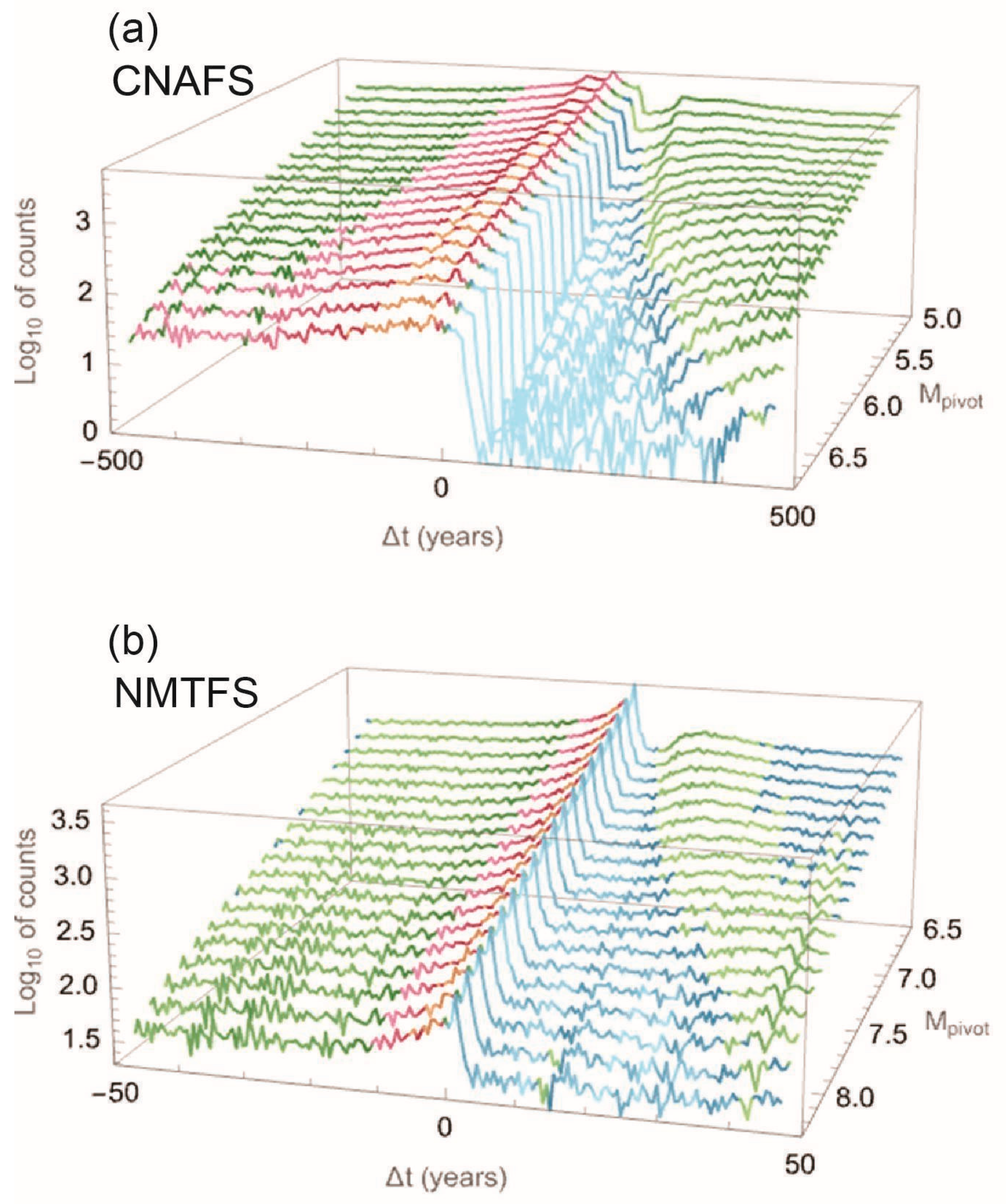
The expected time variations of the stress on the seismogenic structures are consistent with the elastic-rebound model and are clearly visible in Figure 2 for both geodynamic contexts. Other significant features are put in evidence by the stacking procedure applied to the number of events preceding and following the pivot events on a long-term scale (Figure 3). We explored these features more in detail, letting the magnitude of pivot events change from 5.0 to 6.8 in the analysis concerning the CNAFS and from 6.5 to 8.3 for the NMTFS. Figure 5 (notice the number of events in the logarithmic scale) confirms the slow increase in the seismic activity before the pivot event and the oscillations with a decrease in the final precursory stage. The duration of these variations does not depend on Mpivot. Instead, the sudden drop in the seismic activity at the time of the pivot event has a size increase with increasing Mpivot for the CNAFS but not so evident for the NMTFS. Moreover, both in the CNAFS and the NMTFS, the duration of the quiescence period after the pivot events has a clear trend to increase with increasing Mpivot. It can be noted that, in the CNAFS, this quiescence can last up to 400 years for pivot events of magnitude 6.8, which is approximately the magnitude of the main earthquakes historically recorded in this area (Table 1).

Figure 5.
Number of events obtained from the stacking procedure, in logarithmic scale, versus the magnitude of the pivot events for the CNAFS (a) and the NMTFS (b). The color is determined by normalizing each line to its total number of events. This normalization compensates for the decreasing frequency of higher-magnitude pivot events, providing a clearer representation of event trends.
The length of time to recover the standby values of occurrence rates after the transients preceding and following the pivot events increases with increasing Mpivot, as shown in Figure 5.
For a better understanding of the stacking procedure, we show in Video S1 in the Supplementary Materials an animation of the results obtained for the CNAFS with Mpivot = 6.2.
Lastly, our analysis has shown that the seismicity obtained from the simulator, for both the CNAFS and the NMTFS, is characterized by an evident increase in the b-value in the long-term preparation phase of the pivot events, ending just before the pivot event occurrence. This anomalously high b-value is then recovered in a period of the same order of magnitude as the anomaly duration. The decrease in the b-value in the very last bin of the total time interval considered before the pivot event is worth a further investigation, and an in-depth study is underway on this peculiar feature. As a matter of fact, an anomalous low b-value prior to mainshocks has already been regarded as a potential short-term earthquake precursor in the literature (e.g., Montuori et al., 2016 [30]; Papadopoulos et al., 2018 [31]). In a sequence with multiple large events, Gulia and Wiemer (2019) [32] noted the b-value of the aftershocks to be about 10% lower than the background b-value after the first large event of the sequence and recovered its background b-value only after the last large event of the sequence.
We considered seismicity patterns obtained by an identical simulation algorithm applied to two different seismogenic sources, namely a unique large fault system constituted by the subduction interface in Southwestern Japan (NMTFS) and a complex seismogenic system consisting of 43 fault systems with various kinematics in Central Italy (CNAFS). The results of the comparison have shown a striking similarity in the features of the seismicity patterns of the two different geodynamic contexts, except for a relevant difference in their time scale. This similarity derives from the fact that the features of the earthquake catalogues produced by the simulator are controlled by the algorithm adopted in the simulator for the two fault systems in the same way. The faster behavior of the NMTFS compared to that of the CNAFS reflects the ratio between the slip rates of their sources.
We do not have the mechanistic explanations of the seismicity patterns obtained from our simulation algorithm, except for the fact that it behaves as a kind of self-organized system mimicking the vastly more complex real self-organized seismogenic systems.
The question of whether a simulation algorithm reliably represents the real long-term seismogenic process is difficult to answer because the available real observations are of too short a duration to provide significant statistical results. The Italian historical catalogue, even if it is one of the longest in the world, barely contains more than one characteristic earthquake for a single fault system, due to the long average time between two subsequent maximum events generated by the same source (DISS Working Group 2021 [25]).
The circumstance that all four strongest earthquakes reported in Table 1 for the CNAFS in the last 10 centuries occurred in the last 3 centuries, could generate some thoughts on the completeness and homogeneity of the historical catalogue. This circumstance has a probability smaller than 1% of occurring by chance under the hypothesis of a random Poisson time distribution. A test carried out on the 100,000-year simulated catalogue of the CNAFS has shown that a similar clustering effect occurs in an extremely small number of cases and for slightly larger Mth. Therefore, the hypothesis of a variation in the seismicity rate generated by large-scale clustering and a consequence of fault interaction cannot be discarded (in agreement with Console et al., 2022 [15]).
Also, for the historical earthquake catalogue regarding the NMTFS, even if it contains information on some characteristic earthquakes (Parsons et al., 2012 [20]), their limited number, the uncertainty on the fault segments ruptured in each earthquake, and the lack of information about events of a smaller size prevent a significant comparison with the seismicity patterns exhibited by the simulated catalogue.
A possible way of assessing the reliability of simulated catalogues seems to be focusing on short-term seismicity patterns as foreshock sequences and aftershock decay rates, for which the instrumental observations can provide large catalogues going down to small magnitudes. One of these patterns is, for instance, the above-mentioned short-term precursory change in the b-value, which has been observed in real catalogues. A simulation exhibiting this pattern has already been published in Figure 8 of Console et al. (2022) [15]. In line with this, we plan to apply our simulator to seismogenic models based on patches of smaller size, e.g., patches of 0.14 km × 0.14 km, producing earthquakes down to magnitude 2.5, which is well above the completeness magnitude of the Parametric Catalogue of Italian Earthquakes of the last decades (Rovida et al., 2022 [19]). We can estimate that the computer time necessary for a simulation of this kind would be about 1500 times longer than that required for the 100,000 years synthetic catalogue analyzed in this study, i.e., a simulation of 40 years would be feasible employing the same computer resources used for the present work.
Even the most sophisticated earthquake simulators cannot capture all the complexities of real seismic behavior. Despite these limitations, our study encourages further investigation into applying simulators for developing seismogenic models. By focusing on smaller-scale models, the simulator can explore detailed patterns like foreshock sequences, aftershock decay rates, and b-value changes. While computationally demanding, these studies could provide useful insights into earthquake dynamics by comparison with instrumental earthquake catalogues.
Supplementary Materials
The following supporting information can be downloaded at: https://www.mdpi.com/article/10.3390/app14177900/s1, Table S1: Geometric and kinematic parameters of the 198 quadrilateral fault segments derived from the 43 seismogenic sources of DISS v. 3.3.0 (Console et al., 2022 [15]). Table S2: Geometric and kinematic parameters of the 5 large fault segments of the subduction interface (e.g., Parsons et al., 2012 [20]). Video S1: animation of the results obtained by the stacking procedure for the CNAFS with Mpivot = 6.2. Every dot represents the number of events in logarithmic scale in each time bin versus their magnitude.
Author Contributions
All Authors have contributed in equal way to the article. All authors have read and agreed to the published version of the manuscript.
Funding
This research received no external funding.
Informed Consent Statement
Not applicable.
Data Availability Statement
The synthetic catalogues mentioned in this manuscript are available upon request to the Authors.
Conflicts of Interest
The authors declare no conflict of interest.
References
- Rundle, J.B.; Jackson, D.D. Numerical Simulation of Earthquake Sequences. Bull. Seismol. Soc. Am. 1977, 87, 1363–1377. [Google Scholar] [CrossRef]
- Rundle, J.B.; Brown, S. Origin of Rate Dependence in Frictional Sliding. J. Stat. Phys. 1991, 65, 403–412. [Google Scholar] [CrossRef]
- Ward, S.N. An Application of Synthetic Seismicity in Earthquake Statistics: The Middle America Trench. J. Geophys. Res. 1992, 97, 6675–6682. [Google Scholar] [CrossRef]
- Ward, S.N. A Synthetic Seismicity Model for Southern California: Cycles, Probability and Hazard. J. Geophys. Res. 1996, 101, 2293–22418. [Google Scholar] [CrossRef]
- Ward, S.N. San Francisco Bay Area Earthquake Simulations: A Step towards a Standard Physical Earthquake Model. Bull. Seismol. Soc. Am. 2000, 90, 370–386. [Google Scholar] [CrossRef]
- Ward, S.N. ALLCAL Earthquake Simulator. Seismol. Res. Lett. 2012, 83, 964–972. [Google Scholar] [CrossRef]
- Tullis, T.E. Generic Earthquake Simulator. Preface to the Focused Issue on Earthquake Simulators. Seismol. Res. Lett. 2012, 83, 957–958. [Google Scholar] [CrossRef]
- Wilson, J.M.; Yoder, M.R.; Rundle, J.B.; Turcotte, D.L.; Schultz, K.W. Spatial Evaluation and Verification of Earthquake Simulators. Pure Appl. Geophys. 2017, 174, 2279–2293. [Google Scholar] [CrossRef]
- Shaw, B.E.; Milner, K.R.; Field, E.H.; Richards-Dinger, K.; Gilchrist, J.H.; Dieterich, J.H.; Jordan, T.H. A Physics-Based Earthquake Simulator Replicates Seismic Hazard Statistics across California. Sci. Adv. 2018, 4, eaau0688. [Google Scholar] [CrossRef]
- Schultz, K.W.; Sachs, M.; Yoder, M.R.; Rundle, J.B.; Turcotte, D.L.; Helen, E.M.; Donnellan, A. Virtual Quake: Statistics, Co-Seismic Deformations and Gravity Changes for Driven Earthquake Fault Systems. In International Symposium on Geodesy for Earthquake and Natural Hazards (GENAH); Hashimoto, M., Ed.; Springer: Cham, Switzerland, 2015. [Google Scholar]
- Christophersen, A.; Rhoades, D.A.; Colella, H.V. Precursory Seismicity in Regions of Low Strain Rate: Insights from a Physics-Based Earthquake Simulator. Geophys. J. Int. 2017, 209, 1513–1525. [Google Scholar] [CrossRef]
- Field, E.H. Computing Elastic-Rebound-Motivated Earthquake Probabilities in Unsegmented Fault Models: A New Methodology Supported by Physics-Based Simulators. Bull. Seismol. Soc. Am. 2015, 105, 544–559. [Google Scholar] [CrossRef]
- Field, E.H. How Physics-Based Earthquake Simulators Might Help Improve Earthquake Forecasts. Seismol. Res. Lett. 2019, 90, 467–472. [Google Scholar] [CrossRef]
- Rundle, J.B.; Stein, S.; Donnellan, A.; Turcotte, D.L.; Klein, W.; Saylor, C. The Complex Dynamics of Earthquake Fault Systems: New Approaches to Forecasting and Nowcasting of Earthquakes. Rep. Prog. Phys. 2022, 84, 076801. [Google Scholar] [CrossRef] [PubMed]
- Console, R.; Vannoli, P.; Carluccio, R. Physics-Based Simulation of Sequences with Foreshocks, Aftershocks and Multiple Main Shocks in Italy. Appl. Sci. 2022, 12, 2062. [Google Scholar] [CrossRef]
- Reid, H.F. The Mechanics of the Earthquake; Carnegie Institution of Washington: Washington, DC, USA, 1910; Volume 2. [Google Scholar]
- Catalli, F. Sorgenti Sismiche: Rappresentazione Matematica Ed Applicazione al Calcolo Degli Spostamenti. In Quaderni di Geofisica; Istituto Nazionale di Geofisica e Vulcanologia: Rome, Italy, 2007; pp. 1–39. ISSN 1590-2595. [Google Scholar]
- Console, R.; Carluccio, R. Earthquake Simulators Development and Application. In Statistical Methods and Modeling of Seismogenesis; Limnios, N., Papadimitriou, E., Tsaklidis, G., Eds.; ISTE, John Wiley: London, UK, 2020; p. 57. [Google Scholar]
- Rovida, A.; Locati, M.; Camassi, R.; Lolli, B.; Gasperini, P.; Antonucci, A. Italian Parametric Earthquake Catalogue (CPTI15), version 4.0 [Data Set]; Istituto Nazionale di Geofisica e Vulcanologia (INGV): Rome, Italy, 2022. [Google Scholar] [CrossRef]
- Parsons, T.; Console, R.; Falcone, G.; Murru, M.; Yamashina, K. Comparison of Characteristic and Gutenberg-Richter Models for Time-Dependent M ≥ 7.9 Earthquake Probability in the Nankai-Tokai Subduction Zone, Japan. Geophys. J. Int. 2012, 190, 1673–1688. [Google Scholar] [CrossRef]
- Yamamoto, Y.; Yada, S.; Ariyoshi, K.; Hori, T.; Takahashi, N. Seismicity Distribution in the Tonankai and Nankai Seismogenic Zones and Its Spatiotemporal Relationship with Interplate Coupling and Slow Earthquakes. Prog. Earth Planet. Sci. 2022, 9, 32. [Google Scholar] [CrossRef]
- Hanks, T.C.; Kanamori, H. A Moment Magnitude Scale. J. Geophys. Res. 1979, 84, 2348–2350. [Google Scholar] [CrossRef]
- Vannoli, P.; Burrato, P.; Fracassi, U.; Valensise, G. A Fresh Look at the Seismotectonics of the Abruzzi (Central Apennines) Following the 6 April 2009 L’Aquila Earthquake (Mw 6.3). Ital. J. Geosci. 2012, 131, 309–329. [Google Scholar] [CrossRef]
- Vannoli, P.; Vannucci, G.; Bernardi, F.; Palombo, B.; Ferrari, G. The Source of the 30 October 1930, Mw 5.8, Senigallia (Central Italy) Earthquake: A Convergent Solution from Instrumental, Macroseismic and Geological Data. Bull. Seismol. Soc. Am. 2015, 105, 1548–1561. [Google Scholar] [CrossRef]
- DISS Working Group. Database of Individual Seismogenic Sources (DISS), Version 3.3.0: A Compilation of Potential Sources for Earthquakes Larger Than M 5.5 in Italy and Surrounding Areas; Istituto Nazionale di Geofisica e Vulcanologia (INGV): Rome, Italy, 2021. [Google Scholar] [CrossRef]
- Di Bucci, D.; Vannoli, P.; Burrato, P.; Fracassi, U.; Valensise, G. Insights from the Mw 6.3, 2009 L’Aquila Earthquake (Central Apennines) to Unveil New Seismogenic Sources through Their Surface Signature: The Adjacent San Pio Fault. Terra Nova 2011, 23, 108–115. [Google Scholar] [CrossRef]
- Fujiwara, O.; Goto, K.; Ando, R.; Garrett, E. Paleotsunami Research along the Nankai Trough and Ryukyu Trench Subduction Zones—Current Achievements and Future Challenges. Earth-Sci. Rev. 2023, 210, 103333. [Google Scholar] [CrossRef]
- Meade, B.J. Kinematic Earthquake Sequences on Geometrically Complex Faults. arXiv 2023, arXiv:2304.06797. [Google Scholar]
- Shi, Y.; Bolt, B.A. The Standard Error of the Magnitude-Frequency b Value. Bull. Seismol. Soc. Am. 1982, 72, 1677–1687. [Google Scholar] [CrossRef]
- Montuori, C.; Murru, M.; Console, R. Spatial Variation of the B-Value Observed for the Periods Preceding and Following the 24 August 2016, Amatrice Earthquake (ML6.0) (Central Italy). Ann. Geophys. 2016, 59. [Google Scholar] [CrossRef]
- Papadopoulos, G.; Minadakis, G.; Orfanogiannaki, K. Short-Term Foreshocks and Earthquake Prediction. In Pre-Earthquake Processes: A Multidisciplinary Approach to Earthquake Prediction Studies; Ouzounov, D., Pulinets, S., Hattori, K., Taylor, P., Eds.; Geophysical Monograph Series; AGU Publications: Washington, DC, USA, 2018. [Google Scholar] [CrossRef]
- Gulia, L.; Wiemer, S. Real-Time Discrimination of Earthquake Foreshocks and Aftershocks. Nature 2019, 574, 193–199. [Google Scholar] [CrossRef]
Disclaimer/Publisher’s Note: The statements, opinions and data contained in all publications are solely those of the individual author(s) and contributor(s) and not of MDPI and/or the editor(s). MDPI and/or the editor(s) disclaim responsibility for any injury to people or property resulting from any ideas, methods, instructions or products referred to in the content. |
© 2024 by the authors. Licensee MDPI, Basel, Switzerland. This article is an open access article distributed under the terms and conditions of the Creative Commons Attribution (CC BY) license (https://creativecommons.org/licenses/by/4.0/).