Article

Fast and Nondestructive Proximate Analysis of Coal from Hyperspectral Images with Machine Learning and Combined Spectra-Texture Features

1
College of Geoscience and Surveying Engineering, China University of Mining and Technology Beijing, Beijing 100083, China
2
State Key Laboratory for Fine Exploration and Intelligent Development of Coal Resources, China University of Mining and Technology, Xuzhou 221116, China
3
Inner Mongolia Research Institute, China University of Mining and Technology Beijing, Ordos 017004, China
*
Author to whom correspondence should be addressed.
Appl. Sci. 2024, 14(17), 7920; https://doi.org/10.3390/app14177920
Submission received: 25 July 2024 / Revised: 27 August 2024 / Accepted: 29 August 2024 / Published: 5 September 2024
(This article belongs to the Section Optics and Lasers)

Abstract

:
Proximate analysis, including ash, volatile matter, moisture, fixed carbon, and calorific value, is a fundamental aspect of fuel testing and serves as the primary method for evaluating coal quality, which is critical for the processing and utilization of coal. The traditional analytical methods involve time-consuming and costly combustion processes, particularly when applied to large volumes of coal that need to be sampled in massive batches. Hyperspectral imaging is promising for the rapid and nondestructive determination of coal quality indices. In this study, a fast and nondestructive coal proximate analysis method with combined spectral-spatial features was developed using a hyperspectral imaging system in the 450–2500 nm range. The processed spectra were evaluated using PLSR, with the most effective MSC spectra selected. To reduce the spectral redundancy and improve the accuracy, the SPA, Boruta, iVISSA, and CARS algorithms were adopted to extract the characteristic wavelengths, and 16 prediction models were constructed and optimized based on the PLSR, RF, BPNN, and LSSVR algorithms within the Optuna framework for each quality indicator. For spatial information, the histogram statistics, gray-level covariance matrix, and Gabor filters were employed to extract the texture features within the characteristic wavelengths. The texture feature-based and combined spectral-texture feature-based prediction models were constructed by applying the spectral modeling strategy, respectively. Compared with the models based on spectral or texture features only, the LSSVR models with combined spectral-texture features achieved the highest prediction accuracy in all quality metrics, with R p 2 values of 0.993, 0.989, 0.979, 0.948, and 0.994 for Ash, VM, MC, FC, and CV, respectively. This study provides a technical reference for hyperspectral imaging technology as a new method for the rapid, nondestructive proximate analysis and quality assessment of coal.

1. Introduction

Coal is a major source of energy in China and globally. In 2022, the total global demand for coal was 8415 million tons, while in China alone, it was 4520 million tons, accounting for 53.7% of the total demand [1]. With the enormous demand for coal, the market is paying more attention to the quality of coal. The different characteristics of coal are usually crucial for coal mining, utilization, and research processes for pollution issues [2,3]. Therefore, accurately characterizing the quality of coal correctly is essential before coal can be utilized. Coal is a complex assemblage of inorganic and organic materials, formed by coal metamorphism, and its quality is influenced by coal lithology, elements, organic matter, and mineral assemblages [3]. Coal proximate analysis can be defined as a technique that measures ash, volatile matter, moisture, and fixed carbon content [4], and is the most commonly used method to characterize coal quality. The calorific value of coal is also included in this study, with a total of five indicators, which is relevant to coal utilization and trade.
Currently, traditional proximate analysis of coal primarily relies on the chemical processes of combustion, with indicators based on the percentage of mass lost. Moisture content is measured first, as it is the initial component eliminated when coal is heated (105–110 °C) (ISO11722) [5]. Volatile matter is recorded as an indicator of the decomposition of substances when coal is heated to high temperatures (900 °C) for approximately 7 min (ISO 562) [6]. Ash is finally measured as the residue after the coal has been combusted to a constant mass at the final temperature (815 °C) (ISO 1171) [7]. Finally, fixed carbon is the remaining material in the fuel after the former three components have been determined. Calorific value indicates the energy produced by the complete combustion of coal [8]. Although these methods are highly accurate, they need to consume coal, which causes loss. Additionally, a large number of sampling tests are mandatory when there is a large amount of coal, which is even more time-consuming and laborious [9].
Spectroscopic analysis has been widely used in many fields for the qualitative and quantitative characterization of substances by measuring the reflectance or absorbance of spectra [10,11,12]. Previous studies have demonstrated that moisture, ash, volatile matter, and other components of coal can be determined using NIR spectroscopy. Andres et al. used NIR spectroscopy to classify and predict ash, volatile matter, moisture, fixed carbon, and calorific value of coal samples by partial least-squares regression [13,14,15]. Le et al. analyzed NIR spectroscopy in 350–2500 nm using a convolutional neural network and achieved an RMSE of 1.75%, 2.27%, and 0.64 J/g for the determination of coal ash, volatile matter, and low heating value, respectively [16]. For coal calorific value, Begum et al. developed two gross calorific value (GCV) prediction models based on NIR spectra and coal properties. Their comparison revealed that the model based on spectral reflectance provided more accurate predictions, with an R 2 of 0.92 [17]. In addition, Begum et al. also analyzed the spectral characteristics of coal and conducted a comprehensive prediction of ash, moisture, volatile matter, fixed carbon, and the calorific value of coal [18]. Raman spectroscopy (RS), laser-induced breakdown spectroscopy (LIBS), and Fourier transform infrared (FTIR) spectroscopy have also been used to analyze coal [19,20,21]. Gomez et al. developed a PLS calibration model based on FTIR to predict the fixed carbon, calorific value, ash, and volatile matter of coal [22]. Zhang et al. implemented the proximate and elemental analysis of coal based on LIBS by combining spectral normalization with PLSR and SVR, respectively [23]. Regarding the molecular composition of coal, Matlala et al. utilized Raman spectroscopy to analyze the macromolecular structure of coal and its flotation products, which is valuable for predicting the behavior of coal in industrial applications [24]. The analytical performance of these techniques is similar to that of NIR spectroscopy, but all of them still have potential for further improvement. Therefore, new explorations are necessary to achieve more accurate spectral analysis of coal. Moreover, coal quality indicators can be influenced not only by spectral reflectance but also by coal texture. For example, coal with varying ash and volatile matter content often exhibits differences in hardness and color. However, most research has focused on investigating the spectra of coal and has not attempted to develop a coal quality detection model using texture information.
Hyperspectral imaging (HSI) has the advantages of simultaneous spectral capture and image acquisition, enabling the expansion of information from spectral to spatial dimensions [25]. HSI can implement the rapid and nondestructive detection of substances and visualize the spatial distribution, which is of great significance for on-line monitoring in many fields, such as industrial production [26] and medical detection [27]. Texture features, as an important representation of spatial information, can be combined with spectral information to achieve more effective object characterization. Guo et al. extracted texture features from wheat stripe rust samples by using a grayscale covariance matrix (GLEM) and constructed a good recognition model [28]. Wang et al. achieved the accurate classification of maize seeds from different years using histogram statistics (HS) and GLEM texture features extracted from hyperspectral images [29]. Hashim et al. extracted texture features from reflectance images of bananas using Gabor filters (Gabor), wavelet transforms, and the Tamura method and analyzed their performance in assessing the quality of bananas [30]. However, as far as we know, there is no study that attempts to apply the combined spectral-textural features of hyperspectral data for coal proximate analysis and the visualization of coal quality indicators.
In conclusion, near-infrared spectroscopy can be used for the proximate analysis of coal. However, studies on the effect of coal’s spatial information on proximate analysis remain insufficient, and the research on combining spectra and texture features for coal analysis has not yet been involved, and has not obtained a high accuracy. Therefore, the objective of this study is to investigate the feasibility of combining spectral-spatial features from hyperspectral images for predicting coal quality indices, thereby providing technical references for rapid and nondestructive coal proximate analysis.

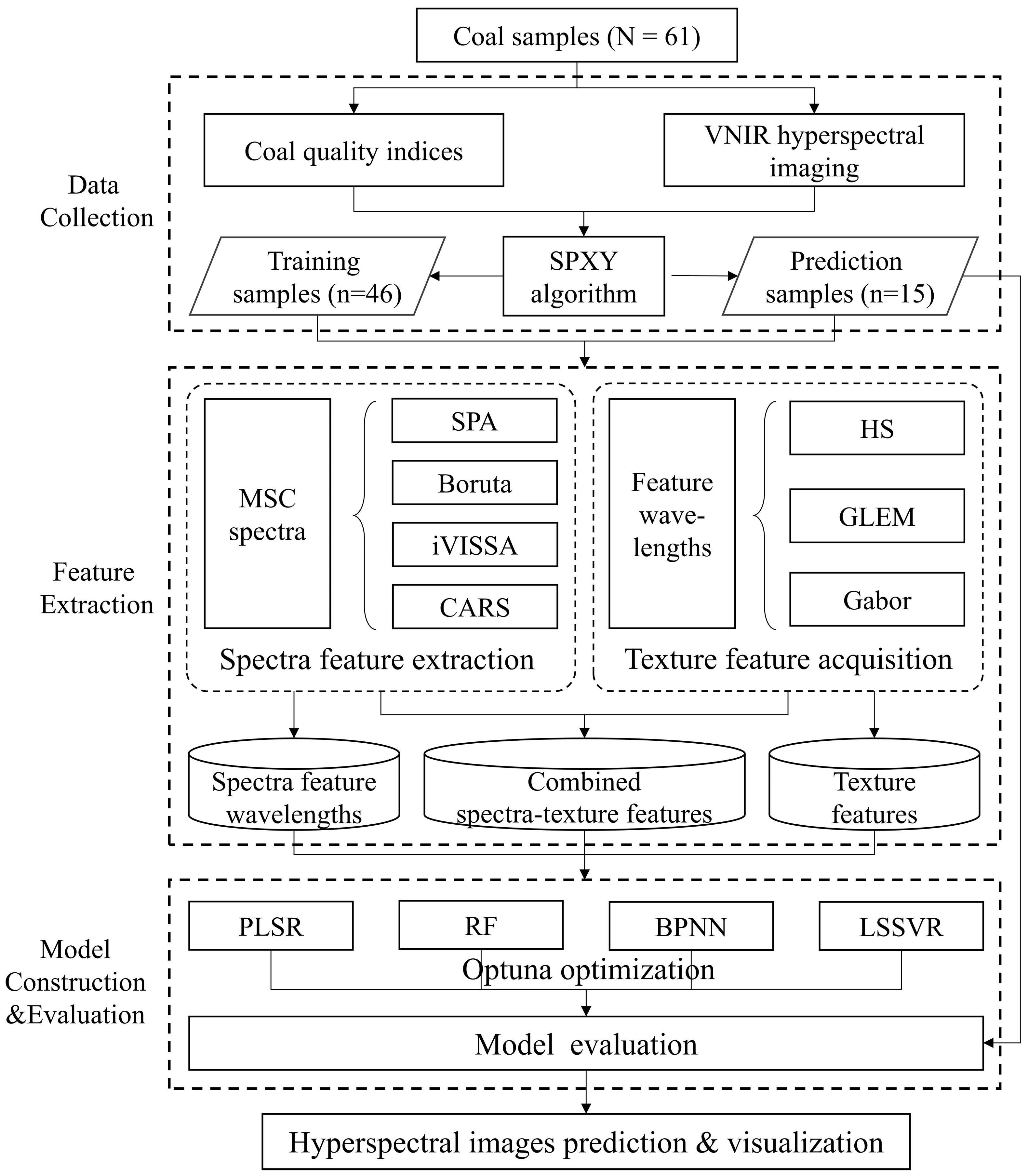
2. Materials and Methods

In this study, 61 coal samples were meticulously prepared for analysis. For data collection, the coal quality indices of all samples were determined using traditional methods, and their corresponding hyperspectral images were acquired. To construct and evaluate the prediction model for coal quality indices, the dataset was divided into training and prediction sets using SPXY algorithm with a ratio of 3:1. During feature extraction, MSC spectra were employed to obtain feature wavelengths using four different methods. Based on these extracted feature wavelengths, the coal texture features were acquired through three approaches. Additionally, combined spectra-texture features of coal were accessed by merging the extracted spectra feature wavelengths and texture features. Finally, using the spectra feature wavelengths, texture features, and combined spectra-texture features, prediction models for each coal quality indicator were developed by applying four machine learning algorithms optimized within the Optuna framework. These optimal models were then evaluated with the prediction set and subsequently employed on the hyperspectral images to visualize the coal quality indices distribution. The research flow of the study is shown in Figure 1.

2.1. Sample Preparation

The coal materials used in this study were collected in Pucheng City, Shanxi Province, China. A total of 61 coal samples were analyzed, comprising two types: anthracite and bituminous coal. The primary difference between these two types lies in their volatile content, with bituminous coal containing the majority. It has been shown that the particle size of coal can affect the spectra reflectance; within a certain range, the coal particle size decreases, the spectra reflectance increases [31]. However, the spatial information of coal with a smaller particle size (e.g., 0.2 mm) is relatively poor. Therefore, to enhance the spectral reflectance and utilize the spatial information of coal, a toothed-roll crusher (Haoxin DG200*150, Ganzhou, China) was employed to reduce the coal size from 50 mm to approximately 3 mm. The crushed coal was dried and sieved using a 3 mm diameter mesh screen and divided into two parts, one for testing and the other for acquiring hyperspectral image data.
The proximate analysis of the 61 coal samples included moisture content (MC, %), ash content (Ash, %), volatile matter (VM, %), fixed carbon (FC, %), and coal calorific value (CV, MJ/kg). The first four indices of coal were determined according to the Chinese standard GB/T 212-2008 [32], which aligns with ISO 11722 (MC), ISO 1171 (Ash), and ISO 562 (VM and FC). The fixed carbon was determined as Equation (1). The calorific value (CV) of coal was determined in the laboratory using an oxygen bomb calorimeter according to GB/T 213-2008 [33].
F C = 100 % A s h M C V M

2.2. Hyperspectral Image Collection

2.2.1. Image Acquisition

The hyperspectral images of coal were collected using the HySpex series of HSI spectrometers (Norsk Elektro Optikk A/S) including VNIR-1800 with wavelengths from 405 to 995 nm and SWIR-384 with wavelengths from 953 to 2517 nm. The system is mainly composed of a mobile platform, twelve halogen lamps, and two HySpex spectrometers in which the wavelength range is divided into 186 and 288 spectral bands at 405–995 nm and 953–2517 nm, respectively. The raw image acquired by the HSI spectrometers is actually the signal intensity of the sensors. Therefore, the dark and white reference image are required to calibrate the raw image to reflectance data. During hyperspectral data acquisition, the white reference image was captured under identical conditions to the coal raw image by using a homogeneous, stable, and highly reflective white plate (MFB99-006Y, Anhui Institute of Optics and Precision Machinery, Hefei, China) as the calibration reference material. To eliminate the effects of dark current from the imaging sensors, the dark reference image was obtained with the light source turned off and the camera lens fully covered by a non-reflective opaque cover. After hyperspectral data acquisition, reflectance calibration was performed according to Equation (2):
R = D N S D N D D N W D N D
where R∈[0,1], D N D represents the dark reference image value, D N W represents the white reference image value, and D N S is the coal raw image value. The pseudo-color images of four randomly selected coal samples are shown in Figure 2.

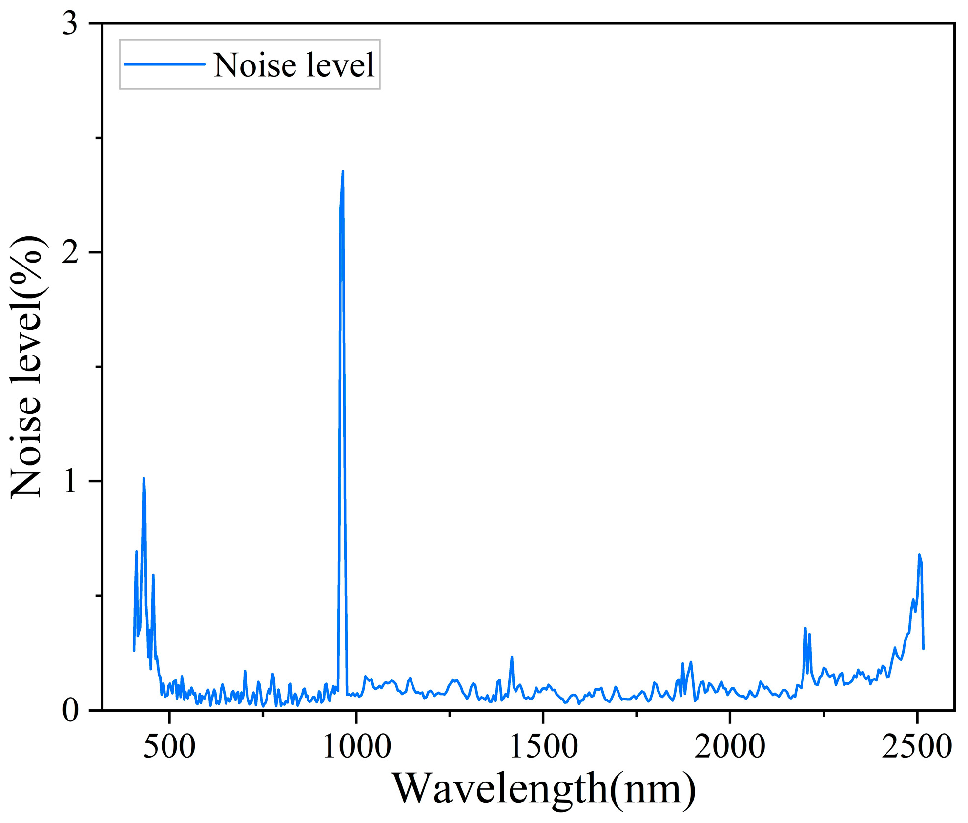
2.2.2. Data Preprocessing

A region of interest (ROI) of the same size was selected at the same location in the hyperspectral image of each coal sample to obtain the coal spectra. A mask was created based on the spectral difference between the coal and the background, allowing for the extraction of the coal sample region and the exclusion of background influences. Figure 3 illustrates the reflectance spectra of 61 coal samples derived by averaging all pixels within the ROI and the characteristic wavelengths associated with the coal quality indices. Meanwhile, Table 1 lists the characteristic wavelengths and the corresponding groups or ions in the coal proximate analysis which are consistent with Figure 3.
To filter the analyzed wavelengths, the noise level at each wavelength was evaluated by calculating a noise level vector [37]. Suppose that there are m coal samples, and the length of spectral data for each sample is n . Thus, the spectral data of these coal samples form an m × n matrix. The spectra noise level is an n -dimensional vector, calculated using Equations (3)–(5):
R n o i s e = M e d i a n c o l R R a w R S G
R r e f e r = M e a n c o l R R a w
N o i s e   l e v e l = R n o i s e R r e f e r
where R S G is an m × n matrix representing the spectra after denoising using SG filtering with a window size of five points and a second-degree polynomial. R R a w represents the original spectra matrix of size m × n . R n o i s e represents the spectra noise vector of n dimensions, obtained by computing the absolute value of the difference between R R a w and R S G , followed by column-wise median calculation. R r e f e r is the n-dimensional reference spectra obtained by averaging R R a w in the column direction. N o i s e   l e v e l is an n -dimensional vector that reflects the quality of each wavelength.
As shown in Figure 4, most wavelengths exhibit low noise ratios of less than 0.5%. The wavelengths with higher noise ratios are located at <465 nm, 954–975 nm, and >2470 nm, where the noise ratios are close to or exceed 1%. This occurs because these wavelengths are located at the edge of the spectrometer’s sensing range (<465 nm and >2470 nm) and the overlap of the two sensors (954–975 nm), resulting in a higher noise ratio. Consequently, wavelengths in the range of <465 nm, >2470 nm, and 954–975 nm were excluded from further analysis, while those with a noise level of less than 0.5% were retained for subsequent analysis.

2.3. Data Processing and Modeling Methods

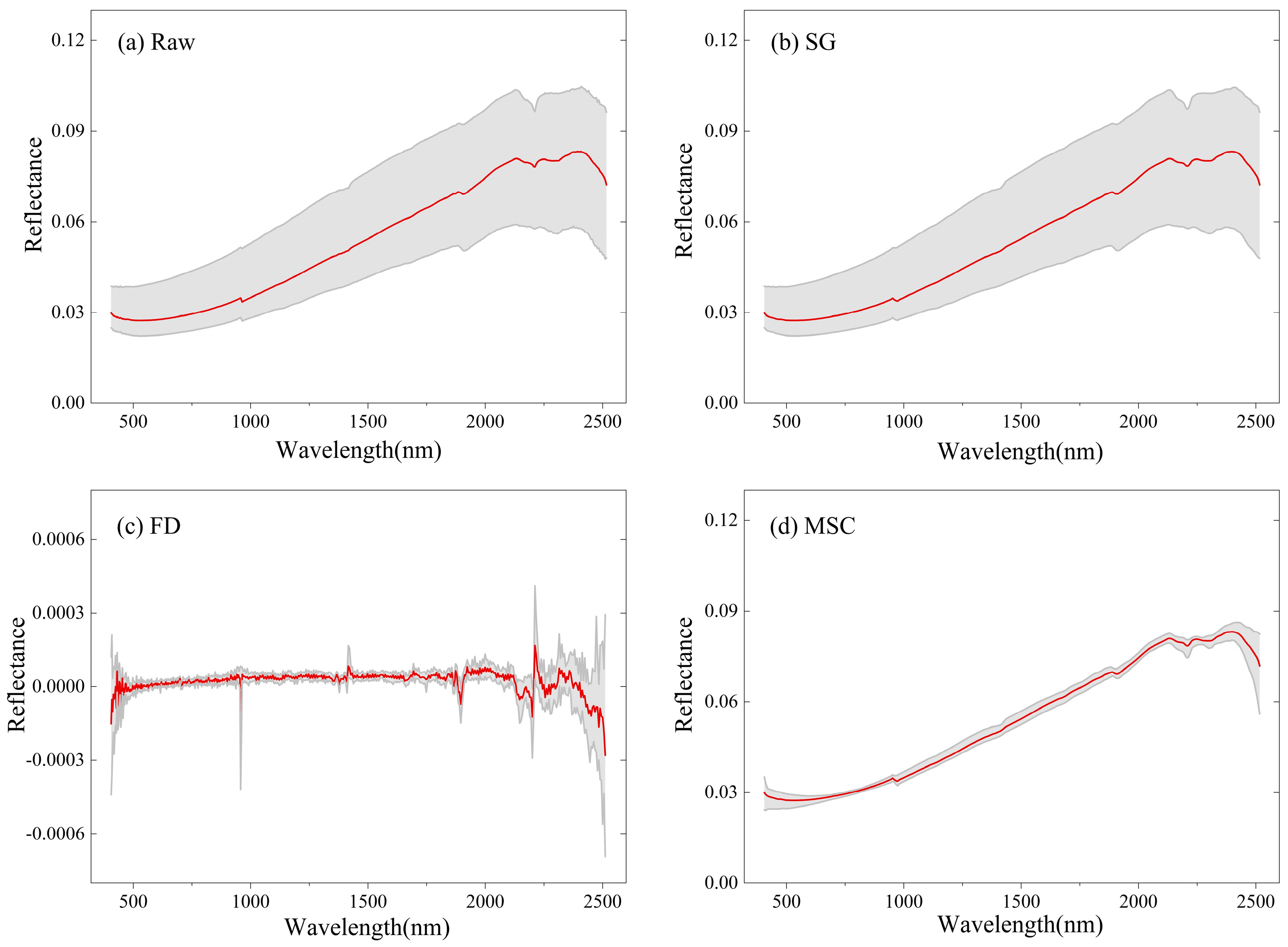
2.3.1. Spectra Data Processing

When utilizing the hyperspectral system for coal imaging, the data will inevitably be affected by factors such as instrument noise, ambient stray light, and uneven coal particles size, which might reduce the accuracy and stability of models. Therefore, processing the spectral data to mitigate these interferences and enhance detection reliability is crucial. In this study, Savitzky–Golay (S–G) convolutional smoothing, first-order derivative (FD), and multiplicative scatter correction (MSC) were mainly used to process the spectra. The S–G can effectively eliminate the instrumental noise, correct the baseline drift, and reduce the interference of the background environment on the spectral data [38]. MSC can eliminate the effect of surface scattering caused by the uneven size of solid particles and the influence of reflective optical path changes on the spectrum, which has a better processing effect in some studies [39].

2.3.2. Feature Wavelengths Selection

The high-dimensionality of hyperspectral data is reflected in the large amount of spatial and spectral information. However, this high-dimensionality imposes a significant burden on computer hardware, rendering it unsuitable for online data acquisition and rapid processing. Selecting representative characteristic wavelengths is crucial to reducing the dimensionality of hyperspectral data, which not only accelerates processing speed and lowers equipment costs but also enhances model accuracy. In this study, four methods are applied to select representative characteristic wavelengths. Successive projection algorithm (SPA) selects a subset of variables with low multicollinearity through stepwise projection and wavelength elimination, which can identify the characteristic wavelengths and reduce redundancy [40]. Competitive adaptive weighted sampling algorithm (CARS) utilizes Monte Carlo sampling and adaptive weighted sampling combined with Partial Least Squares Regression to identify a subset of important variables and select key wavelengths according to their importance levels [41]. Boruta algorithm is a fully correlated feature selection algorithm based on random forest, which can obtain a minimized optimal feature combination by comparing the importance of initial and shadow features [42]. Interval variable iterative space shrinkage approach (iVISSA) achieves the intelligent optimization of the position, width, and combination of the characteristic wavelength intervals by combining the iterations of global and local searches to obtain the indicative wavelength intervals [43].

2.3.3. Extraction of Image Texture Features

The spatial texture information of coal hyperspectral images can partially reflect differences in physical properties (e.g., moisture, cohesion) and chemical properties (e.g., ash content, volatile matter) of coal. To analyze the performance of different texture features for coal quality index determination, three texture extraction methods were implemented on coal hyperspectral data and the results were compared.
Histogram statistics (HS) are commonly utilized in image analysis and processing [44]. In this study, the statistical features of the histogram including mean, variance, skewness, kurtosis, energy, and entropy denoted as HS_M, HS_V, HS_S, HS_K, HS_E1, and HS_E2 were employed as image texture features.
Gray level co-occurrence matrix (GLCM) captures local gray variation characteristics by quantifying the combination and frequency of grayscale values in pixel pairs, thereby describing image texture [45]. In this study, six GLCM texture measures including contrast, dissimilarity, homogeneity, correlation, energy, and entropy were calculated and denoted as GLCM_C1, GLCM_D, GLCM_H, GLCM_C2, GLCM_E1, and GLCM_E2, respectively. The GLCM was extracted with the gray level N = 256 and the distance D = 1. To maintain rotational invariance, the texture information was computed at four orientation angles (θ = 0°, 45°, 90°, 135°) and averaged as the GLCM.
Gabor filter (Gabor) is a linear, frequency, and orientation-selective filter based on a gaussian function modulating a sine wave, and is widely used in texture analysis and feature extraction in computer imaging [46]. Texture features can be extracted by the Gabor filter in various directions and scales. In this study, the Gabor filter calculated the average of the six feature values of contrast, dissimilarity, homogeneity, correlation, energy, and entropy in four directions (θ = 0°, 45°, 90°, 135°). The texture features were obtained using Gabor filters with frequencies F = 0.3, 0.6, 0.9 and denoted as F_C1, F_D, F_H, F_C2, F_E1, and F_E2, respectively.

2.4. Model Development

Models can effectively explore the relationship between variables and targets through transformation, projection, and data mapping, and their performance is affected by different operations. In this study, four algorithms were employed to predict coal quality indicators.
Partial Least Squares Regression (PLSR) is a robust multivariate statistical method widely used in spectroscopic analysis [11,13,15]. It efficiently addresses multicollinearity and high-dimensional data by extracting latent variables that capture the maximum covariance between features and targets. PLSR provides fast learning, good predictive performance, and a strong ability to handle noise and missing data.
Random Forest (RF) is a powerful ensemble learning technique that employs the bagging method to enhance decision tree performance [47]. Bagging methods create multiple data subsets through random sampling and train regression trees on each subset, eventually integrating all the predictions to obtain the final goal. The integrated and stochastic nature of RF contributes to its fast training, robustness to outliers, and strong resistance to overfitting.
Back Propagation Neural Networks (BPNN) are feed forward neural networks based on the back propagation algorithm, which is composed of an input layer, a hidden layer, and an output layer [48]. The neurons in the hidden layer containing weights and biases can capture and represent the complex patterns of the data through nonlinear variations, which is sensitive to the model effect; the learning rate in BPNN controls the updating step of neuron weights to achieve model convergence, which is crucial for model training.
Least Squares Support Vector Regression (LSSVR) is an important regression method based on support vector machines (SVM), characterized by the fast learning speed, strong generalization ability, and simple implementation [39]. The approach simplifies the traditional SVM training process by introducing the least squares loss function, transforming the problem into solving a set of linear equations. The kernel function in LSSVR maps the input data to a high-dimensional space to address nonlinear relationships, which is available with many options such as linear, rbf, etc.

2.5. Model Performance Evaluation

In this study, the data of 61 coal samples were divided into training set (46) and prediction set (15) with the ratio of 3:1. The behavior of machine learning models is significantly influenced by hyperparameters during the training and prediction processes, which greatly affects the results [49]. Manual-based hyperparameter optimization for different models and data requires extensive domain knowledge and often requires a large number of experiments, making it both time-consuming and labor-intensive. The Optuna method applies the tree-structured parzen estimator to perform single-objective optimization, and its hyperparameter combinations are selected based on the estimation of probability distributions, which performs well in high-dimensional and complex search space [50]. With R M S E C V , all models were optimized based on different combinations of input variables and hyperparameters on the training set by 10-fold cross-validation, as shown in Table A1.
The optimized model was trained and validated using leave-one-out cross-validation on the training set and then predicted on the unknown prediction set to comprehensively evaluate model performance. Leave-one-out cross-validation (LOOCV) enables the model to be validated n times (n is the number of samples) across different combinations of samples by taking 1 sample as the validation set and the other (n−1) samples as the training set each time. LOOCV can maximize data usage to comprehensively evaluate the generalization ability of the model and reduce the dependence on specific data features, effectively mitigating the risk of overfitting [51]. This approach is particularly suitable for small datasets [52]. To evaluate the performance of all four models, the coefficient of determination ( R 2 ), the root mean square error ( R M S E ), and the relative prediction deviation ( R P D ) were employed to measure the accuracy of the training and prediction sets, which can be expressed by Equations (6)–(8).
R 2 = 1 i = 1 n y i y i 2 / i = 1 n y i y ¯ 2
R M S E = i = 1 n y i y i 2 / n
R P D = S D R M S E
where y i is the true value, y i is the predicted value, y ¯ is the mean of the measured value, n is the data size, and SD is the validation set standard deviation. Generally, a desirable model should have a high R 2 value and a low R M S E value. The model performance is excellent when R 2 > 0.90 and R P D > 3 [53].
By applying the optimal model to the pixel-by-pixel analysis of coal hyperspectral images, the distribution of coal quality indices is visualized. Specifically, for prediction at each pixel, a mask region centered on the pixel is selected. Then, the features within the region are extracted according to the feature extraction method before and finally imported into the optimal model for the prediction. The predicted values of all pixels are sorted by their original positions to generate a total predicted image. Finally, the maximum and minimum values of this image are used to set the color palette, and the visualization of coal quality indices is produced by assigning colors to the predicted values based on the color palette.

2.6. Shapley Additive Explanations (SHAP)

Machine learning algorithms are often referred to as ‘black boxes’ due to their complex structure, which frequently makes it challenging to explain how accurate predictions are achieved. Explainable artificial intelligence (XAI) [51] methods have important applications for explaining and analyzing the unintelligibility of the predictive causality of machine learning models. The shapely additive interpretation (SHAP) method [54,55], which assesses the importance and contribution of predictor variables based on shape values from game theory, is a key component of XAI and has been utilized in various fields. Due to the localization property of SHAP, SHAP values have the same physical significance as the predicted values, which makes the SHAP values of different models also comparable and additive [56]. To eliminate differences in feature importance caused by the selection of various indicators and to achieve comparable and additive feature importance, the SHAP value is selected as a measure in this experiment from the Python SHAP package (https://github.com/shap/shap/tree/master, accessed on 20 July 2024).

2.7. Software

In this study, the Hyspex hyperspectral images were preprocessed using MATLAB R2018b (MathWorks, Natick, MA, USA), and the spectra of each coal sample were extracted from hyperspectral images using ENVI 5.3 software (Research Systems Inc., Boulder Co., Englewood, CO, USA). Model construction was carried out on PyCharm Community Edition 2023.2 (JetBrains, Prague, Czech Republic) software in a Python 3.8 environment. The PLSR and RF models were implemented using the ‘Scikit-learn’ library (version 0.23.2), and the BPNN model was constructed using ‘Torch’ (version 1.12.0). For the model optimization, the parameter of PLSR was determined using the ‘GridSearchCV’ tool in ‘Scikit-learn’, and the cross-optimization of multiple hyperparameters for the RF, BPNN, and LSSVR was implemented based on the ‘Optuna’ (version 3.6.1) in the Python environment. Finally, the visualization of coal quality indices distribution was also executed using PyCharm Community Edition 2023.2.

3. Results

3.1. Statistics Analysis of Coal Indices Reference

In this study, 61 coal samples were collected and divided into a calibration set (n = 46, 75% of the total samples) and a prediction set (n = 15, 25% of the total samples) using the joint X-Y distance (SPXY). The range, mean, and standard deviation of the coal quality indices are shown in Table 2. As shown in Table 2, the mean ash content for the calibration and prediction sets of coal samples is 36.48% and 34.16%, the mean moisture content is 1.71% and 1.25%, the mean volatile matter is 20.00% and 21.97%, the mean values of fixed carbon content is 41.6% and 43.23%, and the mean values of calorific value content is 19.96 MJ/kg and 21.41 MJ/kg, all of which show no significant deviation. Additionally, the distribution of the calibration set obtained in each coal index is broader than that of the prediction set, which is beneficial for developing an excellent and robust prediction model.

3.2. Spectra Analysis and Preprocessing Results

The raw spectra and the preprocessed spectra of all coal samples are shown in Figure 5. From the raw spectra in Figure 5a, it can be found that the spectral curves of the coal samples have similarity in that they have low reflectance in the visible near infrared (VNIR) band and increased reflectance with the shortwave infrared (SWIR) wavelength. The overall reflectance of coal is low, which is attributed to the black appearance of coal caused by the main carbon component. In addition, the absorption and reflection characteristics of the coal spectral reflectance are generally insignificant, and the more prominent spectral peaks and valleys are mainly concentrated in the shortwave infrared region. There are three obvious spectral reflection peaks at 2100 nm, 2250 nm, and 2400 nm. Additionally, the typical spectral absorption valleys can be clearly observed at 1900 nm, 2200 nm, and 2300 nm. In addition, it can be found that there are weak spectral absorption valleys near 1400 nm, 1700 nm, and 2150 nm. Coal is a complicated, mixed solid material, which mainly contains a large amount of organic matter (e.g., aromatic and aliphatic compounds, etc.) and a small amount of inorganic matter (e.g., SiO2, Al2O3, Fe2O3, etc.) [34,36]. The large amount of organic matter in the coal leads to a more pronounced spectral signature. The typical absorption valley at 2300 nm is consistent with a combination of asymmetric stretching and symmetric bending of CH2 and CH3 [34], while the weak spectral absorption valley at 2150 nm is associated with a combination of aromatic C-H stretching and C-C stretching [35]. In addition, the inorganic components of coal have a great influence on the spectra despite the small amount, and the typical absorption at 1900 nm and the weak absorption feature at 1400 nm are mainly due to the first overtone of O-H in the free water, which is closely related to the moisture content of coal. Clay minerals such as kaolinite, which are the host minerals for the inorganic components of coal [36], form a distinct absorption valley near 2200 nm due to the vibration of Al-OH [35]. However, due to the structural differences between the organic and inorganic components of coal, it is difficult to select the characteristic wavelengths directly by manual operation, so it is necessary to select the characteristic wavelength extraction method to extract the characteristic wavelengths of the suitable spectra.
Figure 5b–d shows the spectra curves after pretreatment by SG, FD, and MSC methods, respectively. Specifically, the SG method reduces noise interference through the polynomial fitting, which makes the spectral curve smoother than Raw while maintaining the spectral characteristics. The FD method applies reflectance differentiation in the wavelength region, which reflects the information of reflectance change and may highlight the spectral features. The MSC can effectively reduce the spectral changes caused by object particle size and uneven distribution, resulting in more concentrated spectral reflectance with sharper features at characteristic reflection peaks and absorption valleys.
The PLSR model was selected to compare the effects of different preprocessing methods using R M S E p as the evaluation metric. The parameters are optimized using 10-fold cross-validation on the training set. Table 3 shows the PLSR modeling results based on the raw spectra and different preprocessed spectra. As shown in Table 3, the prediction accuracy of the SG is generally similar to or better than that of the Raw spectra. However, the spectral heterogeneity due to the coal complex conditions may hinder the effective differentiation of feature wavelengths, potentially leading to model abnormalities, such as the overfitting of OR and SG in MC. FD can emphasize the spectral change information. However, it is significantly affected by noise, which often makes the model unstable in accuracy. In conclusion, MSC achieves the optimal performance across all indices; therefore, this study will be analyzed based on MSC spectra.

3.3. Results of Feature Wavelengths Extracted in Coal Spectra

The results of the characteristic wavelength extraction for coal quality indices are shown in Figure 6. The sensitive characteristic wavelengths for Ash, VM, MC, FC, and CV are 65, 26, 25, 14, and 48, accounting for 14.13%, 5.65%, 5.43%, 3.04%, and 10.43% of the total wavelengths, respectively. The characteristic wavelengths of Ash are particularly concentrated near 750–1050 nm and 2135–2235 nm, where the former can be explained by the absorption due to the transition metal electron jump of Fe2+ and Fe3+ in iron oxides [34], and the latter is primarily due to the absorption of Al-OH in kaolinite and clay minerals [35]. The characteristic wavelengths of VM are more uniformly distributed, mainly observed at 722 nm, 1035 nm, 1430 nm, 1740 nm, 1940 nm, 2160 nm, and 2240 nm, which are associated mainly with C-H stretching and C-C stretching in organics as well as CH2 asymmetric stretching and symmetric bending [35,36]. The characteristic wavelengths of MC are distributed in the range of 500–1000 nm, 1700 nm, 1900 nm, and 2300 nm, which is mainly consistent with the -OH frequency multiplication and H2O vibration [34,35]. FC has only a relatively small number of characteristic wavelengths at 2160 nm, which are related to the combination of aromatic C-H stretching and C-C stretching [35]. The characteristic wavelengths of CV are mainly clustered at 1035 nm, 1440 nm, 1680 nm, 1990 nm, 2200 nm, and 2300 nm.
Table 4 shows the results of the machine learning models based on MSC spectra at different characteristic wavelengths. In terms of feature extraction methods, the number of extracted feature wavelengths among all coal quality indicators is ranked as iVISSA, CARS, Boruta, and SPA, which indicates that the wavelength compression ability of SPA and Boruta is better than that of CARS and iVISSA from the number of wavelengths, which can greatly reduce the pressure of modeling. However, excessive wavelength compression may lead to a loss of effective data information and cut down the model characterization ability. Appropriate wavelength selection can both specialize the feature wavelengths and best characterize the object information, with the characteristic wavelengths selected by CARS fulfilling this requirement effectively. Therefore, it can be found that the optimal models were constructed based on the wavelengths selected by CARS, except for FC, which may be due to the fact that FC is closely related to carbon content which does not have a significant feature in the visible near-infrared band. Considering the R M S E p of the model, it can be found that the LSSVR models usually perform better compared with the other models based on each selected feature wavelength and achieve the optimal prediction of Ash, VM, MC, and CV using the CARS feature wavelengths.
The optimal performance R p 2 of LSSVR is 0.984, 0.971, 0.772, and 0.991 in Ash, VM, MC, and CV, respectively, while the RF model achieves the best accuracy in FC, with an R p 2 of 0.909. The LSSVR model utilizes the optimal decision plane of the high-dimensional mapping data to express the nonlinear relationship of the variables, which can effectively fit the relationship between the reflectance of the characteristic wavelengths and the coal quality indices, and has a faster speed and accuracy in training and prediction compared with other models. Therefore, the subsequent study was conducted based on the LSSVR model under the characteristic wavelengths selected by CARS.

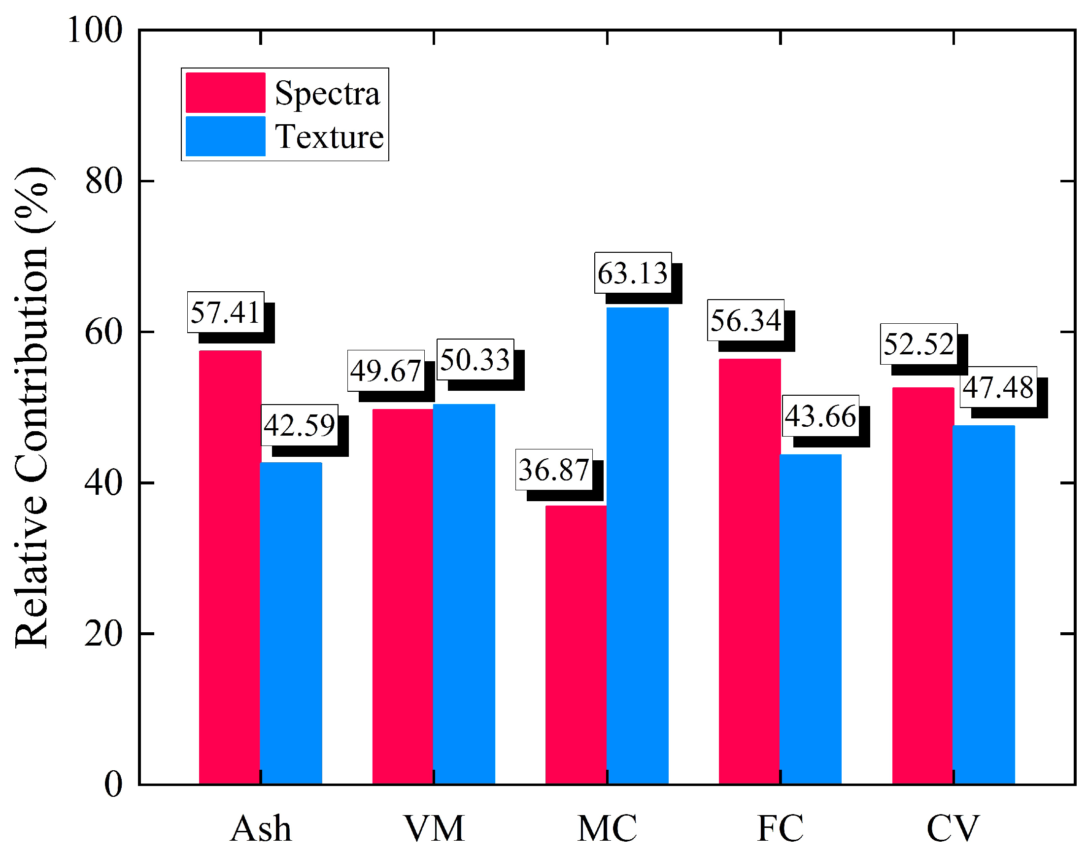
3.4. Results of Combined Features by Wavelengths and Texture Information

Table 5 shows the results of using texture features and combined spectral-texture features to predict coal quality indices. Firstly, the prediction performance of the model utilizing only texture features decreases compared with the results obtained using only spectral features (Table 5). Secondly, the texture features for optimal performance are not uniform among the three texture extraction methods. The Gabor-filtered texture features exhibit the best performance in Ash, VM, and MC, with a prediction set R p 2 of 0.811, 0.927, and 0.957, respectively. In CV, Gabor is also identified as the optimal texture characterization method, primarily due to the minimum R M S E p of 0.994 while excluding the maximum R p 2 of 0.646 from the GLEM. The best model performance for FC was achieved based on the HS features with a prediction set R p 2 of 0.514. This indicates that Ash, VM, and MC have advantages in texture feature-based modeling, which may be related to the fact that these three metrics can reflect the physical attributes of coal and thus affect the texture features. For example, Ash and VM represent the mineral inorganic content and the coalification degree of coal, respectively, which greatly contribute to the coal density [57], grindability [58] and coal color variation, resulting in differences in the texture features of coal images. Variations in MC can also affect the brittleness and strength of coal, altering the coal properties and the external appearance [59]. Among three texture methods, the texture features with the best performance for each index were selected for combined modeling with spectra date. By comparing the model results using texture features and the combined spectral-texture features in Table 5, it can be found that the models combining texture and spectra features have the best performance of accuracy, all of which demonstrate improvement compared with the models based on single spectra or texture features.
The optimal performance of Ash is R p 2 = 0.993, R M S E p = 0.659, R P D = 12.217, reflecting improvements in R p 2 of 0.009 and 0.182 compared with models using only feature wavelengths or texture information. For VM, the optimal performance of VM is R p 2 = 0.989, R M S E p = 0.583, R P D = 9.904, with enhancements of 0.018 and 0.062 in R p 2 . The optimal performance for MC is R p 2 = 0.979, R M S E p = 0.112, R P D = 7.159, and R p 2 improves by 0.207 and 0.022. For FC, the optimal performance is R p 2 = 0.948, R M S E p = 0.838, R P D = 4.544, with R p 2 improving by 0.039 and 0.434. CV shows an optimal performance of R p 2 = 0.994, R M S E p = 0.217, R P D = 13.849, R p 2 improved by 0.003 and 0.375 in spectra and texture features models, respectively. The comparison reveals that MC exhibits greater enhancement, probably due to the fact that moisture is more sensitive to coal texture features. All coal quality indices achieved the best prediction performance in the LSSVR model based on combined spectral-texture features. Figure 7 shows the scatter plots of the optimal model predictions for different coal quality indices. It can be found that the predicted sample points of the model are centrally distributed on the 1:1 line, which indicates that the real value and the predicted value fit well, and the model has excellent prediction. Generally, this paper realizes the accurate prediction of coal quality indices with combined spectral-spatial texture information.

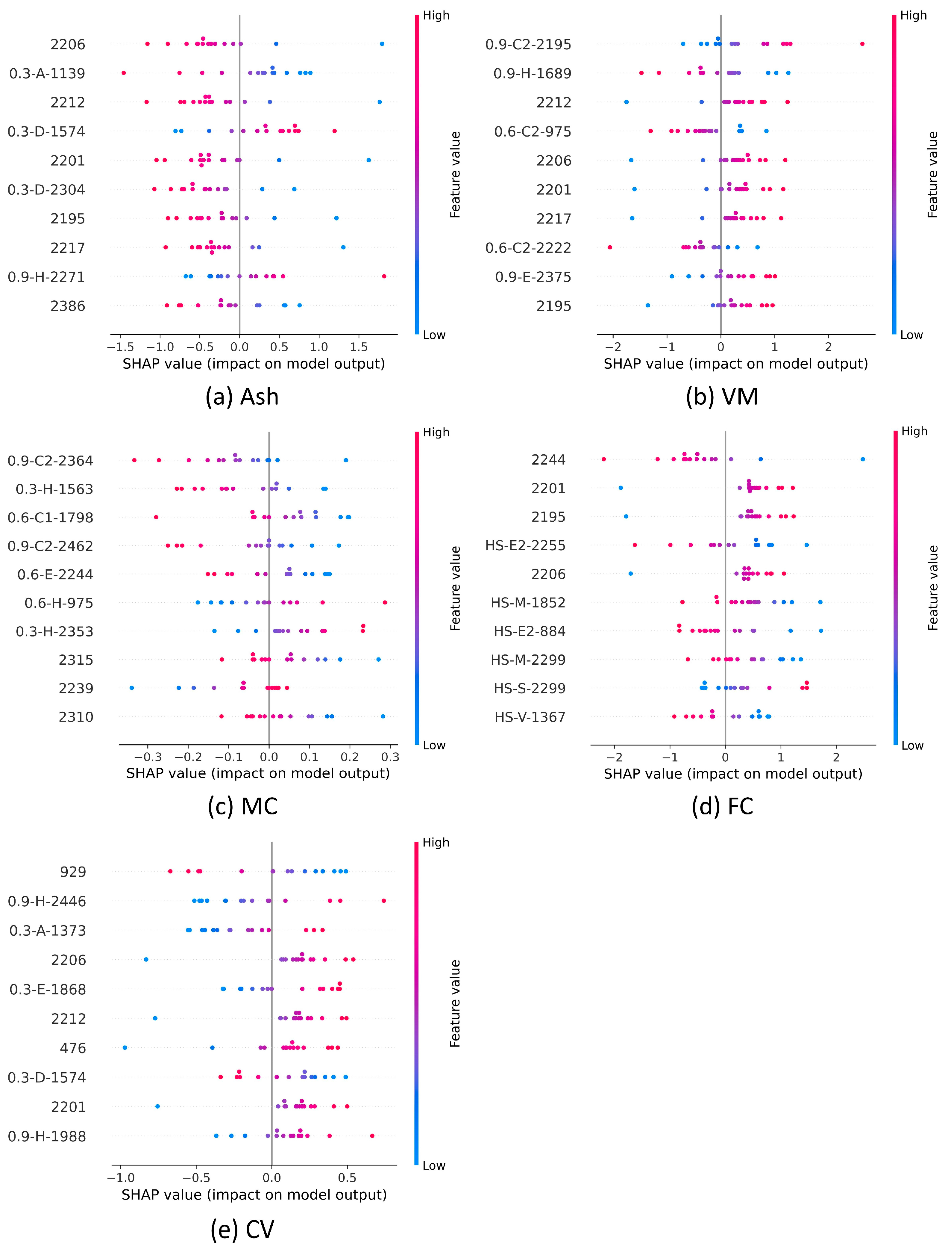
3.5. Influence of Variables on Coal Quality Indices

In order to understand the contribution of spectra and texture features to coal quality indices prediction, SHAP values of different variables were calculated by applying Python’s SHAP library. Figure 8 shows the contribution values of the top 10 variables in coal quality index prediction sorted by importance, where red dots represent higher values and blue dots represent lower values. For instance, Ash can be found to increase with decreasing spectra reflectance at 2206 nm, 2212 nm, 2201 nm, 2195 nm, 2217 nm, and 2386 nm. The typical absorption valley of inorganic minerals such as kaolinite is located near 2200 nm, where lower reflectance indicates a higher inorganic mineral content, which corresponds to increased ash in coal. Figure 9 shows the relative contribution of spectra and texture features in the prediction of coal quality indices calculated from the average absolute SHAP values. As shown in Figure 9, the contribution of spectral features is significant in predicting Ash, FC, and CV, while both spectral and texture features contribute equally to VM. In contrast, the contribution of texture features is much greater than that of spectral features in MC. Section 3.4 reveals that the difference in R p 2 between the model with combined features and the model with spectra features is much smaller for Ash (0.009), VM (0.018), and CV (0.003) than for MC (0.207) and FC (0.039). Therefore, when combining the spectral modeling accuracy (Table 4), variable contributions (Figure 9), and the above analysis, it can be concluded that Ash, VM, and CV can generally achieve high-precision predictions using only spectral features, whereas MC and FC require modeling with combined spectral-texture features. This may be attributed to the two metrics being more sensitive to the textural changes of the coals. These findings could serve as a reference for tasks involving different coal detection requirements.

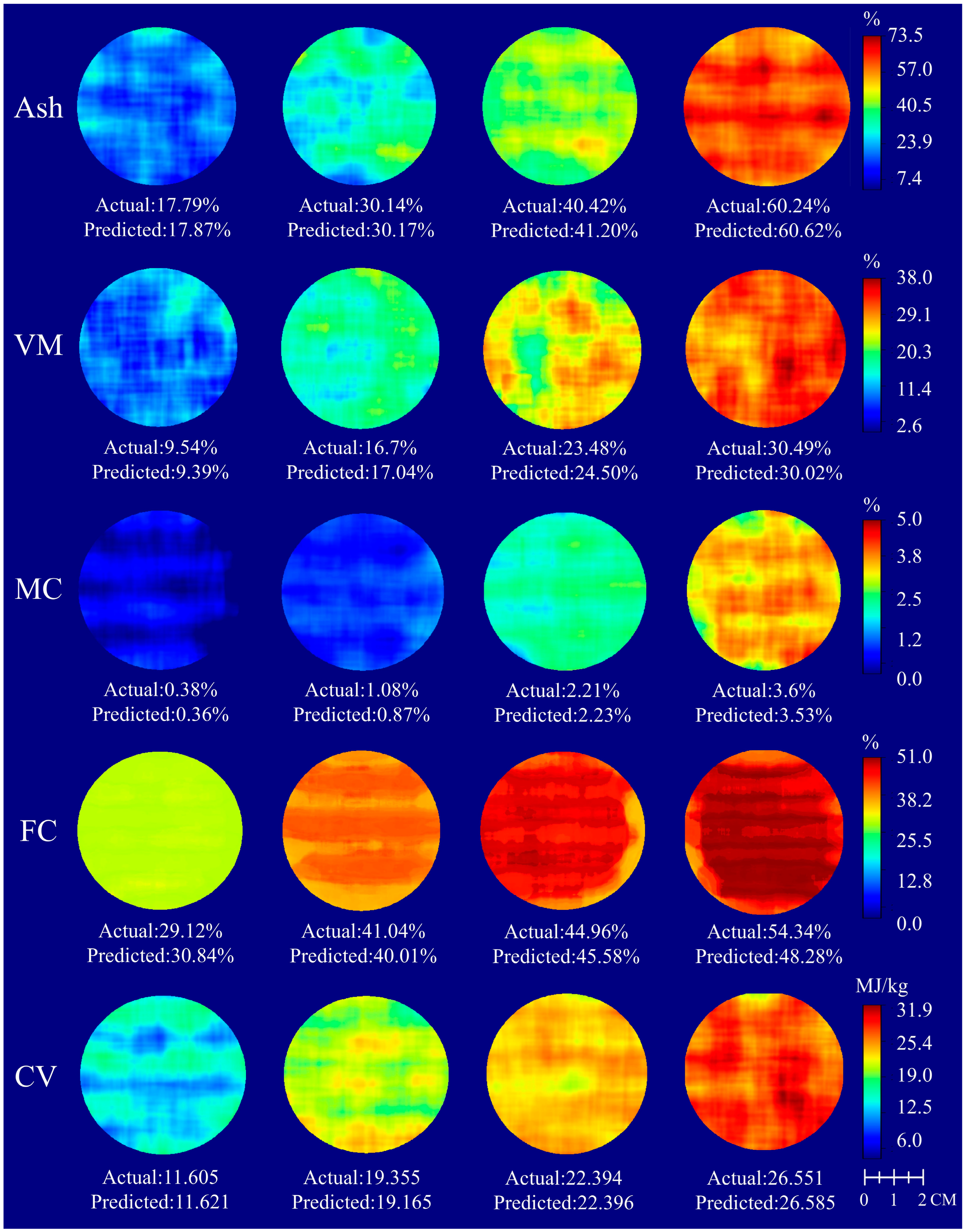
3.6. Visualization of Coal Quality Indices Distribution

The visualization distribution can clearly show the spatial differences of coal quality indices, which can provide an important reference for coal mining, washing and combustion processes. In this study, the LSSVR model with combined spectral feature wavelengths and texture features was employed on coal hyperspectral images to generate gray-scale images of coal quality indices. Samples representing the minimum, 25%, 75%, and maximum values of the dataset were selected for color stretching to illustrate the visual distribution and demonstrate the model’s effectiveness in predicting samples with varying actual values.
The distribution visualization results of coal samples with different quality indices are shown in Figure 10. The color gradient bar denotes the variation range of each indicator and assigns color to the grayscale image. It is evident that the distribution of predicted values for each index is well-balanced, ranging from blue for the minimum value to red for the maximum value, indicating that the model predicts unknown data within a range close to the actual values and exhibits strong generalization ability. Given that the true value range for FC is 29.12–54.34, the minimum value is notably larger than 0 compared with other indices, and its color representation is situated at the upper end of the color gradient bar. Significant variations are observed in the prediction results for samples with different true values, with notable color differences between minimum and maximum value samples. Conversely, the prediction results within each coal sample have small differences with a narrow range of color changes, which indicates that the model can accurately capture the sample characteristics and implement excellent prediction while maximizing the differences between different samples and minimizing the differences between the same samples. The true and predicted values for each sample are closely aligned, with the maximum differences of 0.78%, 1.02%, 0.21%, 6.06%, and 0.19 MJ/kg in Ash, VM, MC, FC, and CV, respectively, which is consistent with the accuracy performance of the model. Overall, the visualization can effectively illustrate spatial differences in coal quality indices and provide valuable technical references for coal mining, processing, and utilization.

4. Discussion

Coal is a complex, inhomogeneous mixture containing both organic and inorganic matters. The proximate analysis of coal is directly related to its quality which has an important role in managing the coal economy, ensuring environmental safety, and promoting resource reutilization. For example, volatile matter, which measures the substances released during the heating process of coal, is composed of gases, low-boiling organic compounds, and tars. This measure reflects the organic compound content in coal [60]. A few volatile organic compounds, such as benzene, toluene, and ethylbenzene, generated from coal combustion, present a significant threat to environment safety and human health due to their toxicity and carcinogenicity [61,62]. In addition, the calorific value, as a measure of coal combustion performance, is critical for the power energy supply and also serves as the primary reference in coal trading. This is particularly relevant for China and India, the two largest coal consumers worldwide, which generated more than 50 percent of their electricity from coal in 2022 [63]. The ash index, which indicates the volume of coal remaining after combustion, is widely used as a waste material in building filling and road repair [64]. Overall, the analysis of coal quality is of considerable importance.
Previous studies have primarily focused on analyzing coal spectral data to achieve proximate analysis of coal quality [13,14,15,16,65]. These studies typically utilize the spectral reflectance of coal obtained from point-based spectrometers, such as the SVC or ASD series [16,18]. Based on the spectral data only, the spectral characteristics of materials related to coal quality indicators have been clarified, but this seems to present a limitation in the further enhancement of the coal proximate analysis. However, the variations in coal quality indices can also alter the physical properties of coal, which may produce different textural information in coal images [57,58,59]. Therefore, this study examines the impact of the texture features of coal images on coal quality indicators to enhance the prediction accuracy of hyperspectral-based models.
The LSSVR model using combined spectral-textural features performed best in predicting coal quality indices, with root-mean-square errors (RMSEs) of 0.112%, 0.659%, 0.583%, 0.838%, and 0.217 MJ/kg for moisture, ash, volatile matter, fixed carbon, and calorific value, respectively. Meanwhile, the relative prediction deviations (RPDs) of all models were much greater than 3, which demonstrated the excellent predictive ability [53]. The results of other work related to this study should be thoroughly analyzed to compare the performance of coal quality indices prediction based on the hyperspectral images and other spectral data. Mondal et al. applied VNIR spectroscopy (400–2500 nm) and PLSR, RF, and XGBoost models to predict the quality indices of 78 coal samples with particle sizes of less than 0.1 mm. The RF regression achieved optimal RMSET of 0.39%, 4.82%, 3.94%, and 2.73 MJ/kg for moisture, ash, volatile matter, and calorific value [31]. The study highlights the modeling advantages of RF, but the predictions performance needs to be further improved compared with our results. Dong et al. implemented the coal quality indices prediction by converting one-dimensional VNIR spectra (350–2500 nm) into two-dimensional data and utilizing a convolutional neural network and a limit learning machine model (DR_TELM). The predicted RMSET of DR_TELM for moisture, ash, volatile matter, fixed carbon, and calorific value were 0.533%, 1.833%. 1.111%, 1.808%, and 0.723 MJ/kg, respectively [66]. Although the convolutional neural network applied to 2D spectra gives it the form of image analysis, it still involves the feature processing of spectra in essence. Compared with our study, their model is a little more complicated, while the performance needs to be further improved. In addition, this study analyzes the importance of variables in prediction models by introducing the SHAP method to quantify the contribution of variables, which is useful for exploring the interpretation of machine learning models with high accuracy. Overall, the visualization method of coal quality indices implemented in this study can better realize the migration of the prediction model from the spectral dimension to the spatial dimension, which offers the advantages of being fast, nondestructive, and accurate compared with the traditional measurement methods.
It should be noted that the quantity and diversity of the sample data still remains the key opportunity to improve the accuracy and robustness of the model. Deep learning models demonstrate significant potential in feature extraction and model construction from hyperspectral data due to their capacity for efficient multi-dimensional data processing and robust nonlinear modeling [66]. In addition, deep learning can also facilitate the development of the end-to-end models, which is highly advantageous for real-world applications [67]. Moreover, further advancement of the method can be widely applied in many promising ways for daily analyses of large quantities of coal. With hyperspectral coal quality testing applied, coal washing plants producing large quantities of commercial coal can avoid quality problems caused by hours of delay in traditional testing methods [68]. In coal trading, coal analysis based on hyperspectral imaging allows the thermal power plants to quantitatively evaluate bulk coal quality during transactions, preventing the adulteration of low-quality coal to stabilize pricing and minimize economic losses [69]. The rapid and accurate determination of coal quality indices is also crucial for energy regulation in coal utilization [70]. In coal-fired power plants, coal blending, which often involves substantial quantities of coal and occurs frequently, could benefit from rapid coal quality analysis, thereby conserving resources and reducing carbon emissions [71].

5. Conclusions

In this study, a fast and nondestructive proximate analysis method for coal based on hyperspectral images is proposed. The SPA, Boruta, iVISSA, and CARS methods are applied to optimize the spectral feature wavelengths based on the MSC spectra. The optimal spectral information-based model for each metric was constructed and evaluated by applying PLSR, RF, BPNN, and LSSVR algorithms. The results show that the CARS-LSSVR model is superior in the prediction of coal quality indices. In the spatial information, the Gabor filtering method and histogram statistics can effectively extract the texture information from the characteristic wavelengths to establish the optimal spatial information-based model. Finally, the optimal prediction model of coal quality indices was constructed by combining the spectral feature wavelengths and texture feature information using the CARS-LSSVR approach. The prediction accuracies were as follows: Ash ( R p 2 = 0.993, R M S E p = 0.659%, R P D = 12.217), VM ( R p 2 = 0.989, R M S E p = 0.583%, R P D = 9.904), MC ( R p 2 = 0.979, R M S E p = 0.112%, R P D = 7.159), FC ( R p 2 = 0.948, R M S E p = 0.838%, R P D = 4.544), and CV ( R p 2 = 0.994, R M S E p = 0.217 MJ/kg, R P D = 13.849). The R p 2 values of the optimal model based on the combined spectral-texture features were improved by 0.009, 0.018, 0.207, 0.039, and 0.003, respectively, as compared with the spectral features. Meanwhile, comparing with the texture features, the R p 2 values were enhanced by 0.182, 0.062, 0.022, 0.434, and 0.375, respectively. In addition, the contributions of spectral and texture features to the model were briefly analyzed by SHAP and suggestions were provided. The results of this study demonstrate that the texture features in coal images can enhance the model performance for predicting coal quality indices. Machine learning coupled with combined spectral-texture features from hyperspectral data can be used to accurately determine coal quality indices, which provides a technical reference for further rapid nondestructive proximate analysis and quality assessment of coal. Future research will focus on expanding the coal sample size and applying deep learning networks to automatically extract hyperspectral features for constructing end-to-end coal quality indicator detection models. The effectiveness of the hyperspectral coal quality determination technique will also be tested in practical application scenarios, such as thermal power plants and coal chemical plants, beyond laboratory settings.

Author Contributions

Conceptualization, J.M. and H.Z.; methodology, H.Z., J.M., and P.W.; software, J.M. and Y.X.; validation, J.M., H.Z., and M.W.; writing—original draft preparation, J.M.; writing—review and editing, H.Z., J.M., Y.Z., Y.S., and Y.X.; visualization, J.M.; project administration, H.Z.; funding acquisition, H.Z. All authors have read and agreed to the published version of the manuscript.

Funding

This research was funded by the National Natural Science Foundation of China Science Foundation Project (41701488), the Open Research Fund of The State Key Laboratory for Fine Exploration and Intelligent Development of Coal Resources, CUMT (SKLCRSM24KF011), the China University of Mining and Technology (Beijing) LongRuan Technology Fund Student Innovation & Enterprise Program (XD2023016004) and the Doctoral Innovative Talents Cultivation Project at China University of Mining and Technology (Beijing) (BBJ2023025).

Institutional Review Board Statement

Not applicable.

Informed Consent Statement

Not applicable.

Data Availability Statement

The data used to support the findings of this study are available from the corresponding author upon request.

Acknowledgments

We thank Hongxing Wang and Xiaodong Li of Shanxi Datang Pucheng coal-fired power plant for supporting us with coal samples. We want to thank all participants and assistants for their support. We also would like to acknowledge the reviewers for their suggestions and comments on the manuscript, which helped us to refine the manuscript and present our findings more clearly.

Conflicts of Interest

The authors declare no conflicts of interest.

Appendix A

Table A1. List of hyperparameters optimized for different models.
ModelsHyperparameter ListRange
PLSRn_compoments[2, min (5, n 1)]
RFn_estimators[55,300] step = 50
max_depth[2,23] step = 1
BPNNInput_dimn
hidden_dimm1
output_dim1
learning_rate[0.001, 0.5]
LSSVRKernel‘linear’, ‘rbf’
C[0.1, 30.0]
Gamma[Sqrt(n)/2, Sqrt(n), Sqrt(n)×2]
1 The parameters: n is the number of input variables, m = (a value is 1–10).

References

  1. IEA. Coal. 2023. Available online: https://www.iea.org/reports/coal-2023 (accessed on 14 August 2024).
  2. Li, D.; Wu, D.; Xu, F.; Lai, J.; Shao, L. Literature overview of Chinese research in the field of better coal utilization. J. Clean. Prod. 2018, 185, 959–980. [Google Scholar] [CrossRef]
  3. Hower, J.C.; Finkelman, R.B.; Eble, C.F.; Arnold, B.J. Understanding coal quality and the critical importance of comprehensive coal analyses. Int. J. Coal Geol. 2022, 263, 104120. [Google Scholar] [CrossRef]
  4. Kiang, Y.-H. Fuel Property Estimation and Combustion Process Characterization: Conventional Fuels, Biomass, Biocarbon, Waste Fuels, Refuse Derived Fuel, and Other Alternative Fuels; Academic Press: London, UK; San Diego, CA, USA, 2018. [Google Scholar]
  5. ISO11722; Solid Mineral Fuels—Hard Coal—Determination of Moisture in the General Analysis Test Sample by Drying in Nitrogen. International Organization for Standardization: Geneva, Switzerland, 2013.
  6. ISO562; Hard Coal and Coke—Determination of Volatile Matter. International Organization for Standardization: Geneva, Switzerland, 2024.
  7. ISO1171; Coal and Coke—Determination of Ash. International Organization for Standardization: Geneva, Switzerland, 2024.
  8. Wang, Z.; Hou, Z.; Zhang, L.; Yao, S.; Sheta, S.; Afgan, M.S. Chapter 21—Coal analysis. In Laser-Induced Breakdown Spectroscopy, 2nd ed.; Singh, J.P., Thakur, S.N., Eds.; Elsevier: Amsterdam, The Netherlands, 2020; pp. 473–498. [Google Scholar] [CrossRef]
  9. Sheta, S.; Afgan, M.S.; Hou, Z.; Yao, S.-C.; Zhang, L.; Li, Z.; Wang, Z. Coal analysis by laser-induced breakdown spectroscopy: A tutorial review. J. Anal. At. Spectrom. 2019, 34, 1047–1082. [Google Scholar] [CrossRef]
  10. Zhao, H.; Wang, M.; Wu, Y.; Mao, J.; Xie, Y.; Jin, Q.; Liu, S.; Tang, G. Fast and nondestructive discrimination of coal types based on spectral feature parameters. Spectrochim. Acta Part A Mol. Biomol. Spectrosc. 2024, 322, 124749. [Google Scholar] [CrossRef]
  11. Bian, X.; Liu, Y.; Zhang, R.; Sun, H.; Liu, P.; Tan, X. Rapid quantification of grapeseed oil multiple adulterations using near-infrared spectroscopy coupled with a novel double ensemble modeling method. Spectrochim. Acta Part A Mol. Biomol. Spectrosc. 2024, 311, 124016. [Google Scholar] [CrossRef] [PubMed]
  12. Bian, X.; Zhao, Z.; Liu, J.; Liu, P.; Shi, H.; Tan, X. Discretized butterfly optimization algorithm for variable selection in the rapid determination of cholesterol by near-infrared spectroscopy. Anal. Methods 2023, 15, 5190–5198. [Google Scholar] [CrossRef]
  13. Andrés, J.M.; Bona, M.T. Analysis of coal by diffuse reflectance near-infrared spectroscopy. Anal. Chim. Acta 2005, 535, 123–132. [Google Scholar] [CrossRef]
  14. Andrés, J.M.; Bona, M.T. ASTM clustering for improving coal analysis by near-infrared spectroscopy. Talanta 2006, 70, 711–719. [Google Scholar] [CrossRef]
  15. Bona, M.T.; Andrés, J.M. Coal analysis by diffuse reflectance near-infrared spectroscopy: Hierarchical cluster and linear discriminant analysis. Talanta 2007, 72, 1423–1431. [Google Scholar] [CrossRef]
  16. Le, B.T.; Xiao, D.; Mao, Y.; He, D. Coal analysis based on visible-infrared spectroscopy and a deep neural network. Infrared Phys. Technol. 2018, 93, 34–40. [Google Scholar] [CrossRef]
  17. Begum, N.; Chakravarty, D.; Das, B.S. Estimation of Gross Calorific Value of Bituminous Coal using various Coal Properties and Reflectance Spectra. Int. J. Coal Prep. Util. 2022, 42, 979–985. [Google Scholar] [CrossRef]
  18. Begum, N.; Maiti, A.; Chakravarty, D.; Das, B.S. Reflectance spectroscopy based rapid determination of coal quality parameters. Fuel 2020, 280, 118676. [Google Scholar] [CrossRef]
  19. Potgieter-Vermaak, S.; Maledi, N.; Wagner, N.; Van Heerden, J.; Van Grieken, R.; Potgieter, J. Raman spectroscopy for the analysis of coal: A review. J. Raman Spectrosc. 2011, 42, 123–129. [Google Scholar] [CrossRef]
  20. Liu, K.; He, C.; Zhu, C.; Chen, J.; Zhan, K.; Li, X. A review of laser-induced breakdown spectroscopy for coal analysis. TrAC Trends Anal. Chem. 2021, 143, 116357. [Google Scholar] [CrossRef]
  21. Ibarra, J.V.; Moliner, R. Coal characterization using pyrolysis-FTIR. J. Anal. Appl. Pyrolysis 1991, 20, 171–184. [Google Scholar] [CrossRef]
  22. Román Gómez, Y.; Cabanzo Hernández, R.; Guerrero, J.E.; Mejía-Ospino, E. FTIR-PAS coupled to partial least squares for prediction of ash content, volatile matter, fixed carbon and calorific value of coal. Fuel 2018, 226, 536–544. [Google Scholar] [CrossRef]
  23. Zhang, Y.; Dong, M.; Cheng, L.; Wei, L.; Cai, J.; Lu, J. Improved measurement in quantitative analysis of coal properties using laser induced breakdown spectroscopy. J. Anal. At. Spectrom. 2020, 35, 810–818. [Google Scholar] [CrossRef]
  24. Matlala, I.V.; Moroeng, O.M.; Kalaitzidis, S.; Wagner, N.J. Raman Spectroscopy for the characterization of the macromolecular structure of Highveld coals (South Africa). Int. J. Coal Geol. 2024, 288, 104531. [Google Scholar] [CrossRef]
  25. Imani, M.; Ghassemian, H. An overview on spectral and spatial information fusion for hyperspectral image classification: Current trends and challenges. Inf. Fusion 2020, 59, 59–83. [Google Scholar] [CrossRef]
  26. Yan, Y.; Ren, J.; Zhao, H.; Windmill, J.F.C.; Ijomah, W.; De Wit, J.; Von Freeden, J. Non-destructive testing of composite fiber materials with hyperspectral imaging—Evaluative studies in the EU H2020 FibreEUse project. IEEE Trans. Instrum. Meas. 2022, 71, 1–13. [Google Scholar] [CrossRef]
  27. Martin, M.E.; Wabuyele, M.B.; Chen, K.; Kasili, P.; Panjehpour, M.; Phan, M.; Overholt, B.; Cunningham, G.; Wilson, D.; DeNovo, R.C. Development of an advanced hyperspectral imaging (HSI) system with applications for cancer detection. Ann. Biomed. Eng. 2006, 34, 1061–1068. [Google Scholar] [CrossRef] [PubMed]
  28. Guo, A.; Huang, W.; Ye, H.; Dong, Y.; Ma, H.; Ren, Y.; Ruan, C. Identification of Wheat Yellow Rust Using Spectral and Texture Features of Hyperspectral Images. Remote Sens. 2020, 12, 1419. [Google Scholar] [CrossRef]
  29. Wang, Z.; Huang, W.; Tian, X.; Long, Y.; Li, L.; Fan, S. Rapid and Non-destructive Classification of New and Aged Maize Seeds Using Hyperspectral Image and Chemometric Methods. Front. Plant Sci. 2022, 13, 849495. [Google Scholar] [CrossRef] [PubMed]
  30. Hashim, N.; Adebayo, S.E.; Abdan, K.; Hanafi, M. Comparative study of transform-based image texture analysis for the evaluation of banana quality using an optical backscattering system. Postharvest Biol. Technol. 2018, 135, 38–50. [Google Scholar] [CrossRef]
  31. Mondal, C.; Pandey, A.; Kumar Pal, S.; Samanta, B.; Dutta, D. Hyperspectral measurement technique based rapid determination of coal quality parameters of Jharia and Raniganj basin coal. Infrared Phys. Technol. 2023, 128, 104504. [Google Scholar] [CrossRef]
  32. GB/T 212-2008; Proximate Analysis of Coal. Standardization Administration of the People’s Republic of China: Beijing, China, 2009.
  33. GB/T 213-2008; Determination of Calorific Value of Coal. Standardization Administration of the People’s Republic of China: Beijing, China, 2009.
  34. Yang, E.; Wang, S.; Ge, S. Study on the Visible and Near-Infrared Spectra of Typical Types of Lump Coal. Spectrosc. Spectr. Anal. 2019, 39, 1717–1723. [Google Scholar] [CrossRef]
  35. Fysh, S.A.; Swinkels, D.A.J.; Fredericks, P.M. Near-Infrared Diffuse Reflectance Spectroscopy of Coal. Appl. Spectrosc. 1985, 39, 354–357. [Google Scholar] [CrossRef]
  36. Van Dyk, J.C.; Benson, S.A.; Laumb, M.L.; Waanders, B. Coal and coal ash characteristics to understand mineral transformations and slag formation. Fuel 2009, 88, 1057–1063. [Google Scholar] [CrossRef]
  37. Liu, C.; Yang, S.X.; Li, X.; Xu, L.; Deng, L. Noise level penalizing robust Gaussian process regression for NIR spectroscopy quantitative analysis. Chemom. Intell. Lab. Syst. 2020, 201, 104014. [Google Scholar] [CrossRef]
  38. Hu, Y.; Huang, P.; Wang, Y.; Sun, J.; Wu, Y.; Kang, Z. Determination of Tibetan tea quality by hyperspectral imaging technology and multivariate analysis. J. Food Compos. Anal. 2023, 117, 105136. [Google Scholar] [CrossRef]
  39. Huang, Z.; Sanaeifar, A.; Tian, Y.; Liu, L.; Zhang, D.; Wang, H.; Ye, D.; Li, X. Improved generalization of spectral models associated with Vis-NIR spectroscopy for determining the moisture content of different tea leaves. J. Food Eng. 2021, 293, 110374. [Google Scholar] [CrossRef]
  40. Xue, H.; Xu, X.; Yang, Y.; Hu, D.; Niu, G. Rapid and Non-Destructive Prediction of Moisture Content in Maize Seeds Using Hyperspectral Imaging. Sensors 2024, 24, 1855. [Google Scholar] [CrossRef]
  41. Zhang, S.; Yin, Y.; Liu, C.; Li, J.; Sun, X.; Wu, J. Discrimination of wheat flour grade based on PSO-SVM of hyperspectral technique. Spectrochim. Acta Part A Mol. Biomol. Spectrosc. 2023, 302, 123050. [Google Scholar] [CrossRef] [PubMed]
  42. Liu, Z.; Lu, Y.; Peng, Y.; Zhao, L.; Wang, G.; Hu, Y. Estimation of Soil Heavy Metal Content Using Hyperspectral Data. Remote Sens. 2019, 11, 1464. [Google Scholar] [CrossRef]
  43. Zhang, R.; Zhang, F.; Chen, W.; Xiong, Q.; Chen, Z.; Yao, H.; Ge, J.; Hu, Y.; Du, Y. A variable informative criterion based on weighted voting strategy combined with LASSO for variable selection in multivariate calibration. Chemom. Intell. Lab. Syst. 2019, 184, 132–141. [Google Scholar] [CrossRef]
  44. Paschos, G.; Petrou, M. Histogram ratio features for color texture classification. Pattern Recognit. Lett. 2003, 24, 309–314. [Google Scholar] [CrossRef]
  45. Arebey, M.; Hannan, M.A.; Begum, R.A.; Basri, H. Solid waste bin level detection using gray level co-occurrence matrix feature extraction approach. J. Environ. Manag. 2012, 104, 9–18. [Google Scholar] [CrossRef]
  46. Gabor, D. Theory of communication. Part 1: The analysis of information. J. Inst. Electr. Eng.—Part III Radio Commun. Eng. 1946, 93, 429–441. [Google Scholar] [CrossRef]
  47. Breiman, L. Random Forests. Mach. Learn. 2001, 45, 5–32. [Google Scholar] [CrossRef]
  48. Peng, Y.; Liu, Z.; Lin, C.; Hu, Y.; Zhao, L.; Zou, R.; Wen, Y.; Mao, X. A New Method for Estimating Soil Fertility Using Extreme Gradient Boosting and a Backpropagation Neural Network. Remote Sens. 2022, 14, 3311. [Google Scholar] [CrossRef]
  49. Pravin, P.S.; Tan, J.Z.M.; Yap, K.S.; Wu, Z. Hyperparameter optimization strategies for machine learning-based stochastic energy efficient scheduling in cyber-physical production systems. Digit. Chem. Eng. 2022, 4, 100047. [Google Scholar] [CrossRef]
  50. Akiba, T.; Sano, S.; Yanase, T.; Ohta, T.; Koyama, M. Optuna: A Next-generation Hyperparameter Optimization Framework. In Proceedings of the 25th ACM SIGKDD International Conference on Knowledge Discovery & Data Mining, Anchorage, AK, USA, 4–8 August 2019. [Google Scholar]
  51. Maxwell, A.E.; Sharma, M.; Donaldson, K.A. Explainable Boosting Machines for Slope Failure Spatial Predictive Modeling. Remote Sens. 2021, 13, 4991. [Google Scholar] [CrossRef]
  52. Zhao, N.; Wu, Z.-S.; Zhang, Q.; Shi, X.-Y.; Ma, Q.; Qiao, Y.-J. Optimization of parameter selection for partial least squares model development. Sci. Rep. 2015, 5, 11647. [Google Scholar] [CrossRef] [PubMed]
  53. Zornoza, R.; Guerrero, C.; Mataix-Solera, J.; Scow, K.M.; Arcenegui, V.; Mataix-Beneyto, J. Near infrared spectroscopy for determination of various physical, chemical and biochemical properties in Mediterranean soils. Soil Biol. Biochem. 2008, 40, 1923–1930. [Google Scholar] [CrossRef] [PubMed]
  54. Lundberg, S.M.; Lee, S.-I. A Unified Approach to Interpreting Model Predictions. arXiv 2017, arXiv:1705.07874. [Google Scholar]
  55. Marcílio, W.E.; Eler, D.M. From explanations to feature selection: Assessing SHAP values as feature selection mechanism. In 2020 33rd SIBGRAPI Conference on Graphics, Patterns and Images (SIBGRAPI), Porto de Galinhas, Brazil, 7–10 November 2020; IEEE: Piscataway, NJ, USA, 2020. [Google Scholar]
  56. Tang, Y.; Duan, A.; Xiao, C.; Xin, Y. The Prediction of the Tibetan Plateau Thermal Condition with Machine Learning and Shapley Additive Explanation. Remote Sens. 2022, 14, 4169. [Google Scholar] [CrossRef]
  57. Mathews, J.P.; Krishnamoorthy, V.; Louw, E.; Tchapda, A.H.N.; Castro-Marcano, F.; Karri, V.; Alexis, D.A.; Mitchell, G.D. A review of the correlations of coal properties with elemental composition. Fuel Process. Technol. 2014, 121, 104–113. [Google Scholar] [CrossRef]
  58. Sengupta, A.N. An assessment of grindability index of coal. Fuel Process. Technol. 2002, 76, 1–10. [Google Scholar] [CrossRef]
  59. Laskowski, J.S. Chapter 3 Coal surface properties. In Developments in Mineral Processing; Elsevier: Amsterdam, The Netherlands, 2001; Volume 14, pp. 31–94. [Google Scholar]
  60. Morley, R.J.; Scaroni, A.W.; Pisupati, S.V.L.N. Coal Utilization. Available online: https://www.britannica.com/technology/coal-utilization (accessed on 14 August 2024).
  61. Zhang, Z.; Yan, X.; Gao, F.; Thai, P.; Wang, H.; Chen, D.; Zhou, L.; Gong, D.; Li, Q.; Morawska, L.; et al. Emission and health risk assessment of volatile organic compounds in various processes of a petroleum refinery in the Pearl River Delta, China. Environ. Pollut. 2018, 238, 452–461. [Google Scholar] [CrossRef]
  62. He, K.; Shen, Z.; Zhang, B.; Sun, J.; Zou, H.; Zhou, M.; Zhang, Z.; Xu, H.; Ho, S.S.H.; Cao, J. Emission profiles of volatile organic compounds from various geological maturity coal and its clean coal briquetting in China. Atmos. Res. 2022, 274, 106200. [Google Scholar] [CrossRef]
  63. EI; BP. Statistical Review of World Energy 2023. Available online: https://www.energyinst.org/statistical-review (accessed on 14 August 2024).
  64. Jayaranjan, M.L.D.; Van Hullebusch, E.D.; Annachhatre, A.P. Reuse options for coal fired power plant bottom ash and fly ash. Rev. Environ. Sci. Bio/Technol. 2014, 13, 467–486. [Google Scholar] [CrossRef]
  65. Gülcan, E.; Gülsoy, Ö.Y.; Can, I.B. Ash content estimation of lignite with visible light and near-infrared sensors. Int. J. Coal Prep. Util. 2020, 40, 438–458. [Google Scholar] [CrossRef]
  66. Xiao, D.; Yan, Z.; Li, J.; Fu, Y.; Li, Z. Rapid proximate analysis of coal based on reflectance spectroscopy and deep learning. Spectrochim. Acta Part A Mol. Biomol. Spectrosc. 2023, 287, 122042. [Google Scholar] [CrossRef] [PubMed]
  67. Zhang, X.; Lin, T.; Xu, J.; Luo, X.; Ying, Y. DeepSpectra: An end-to-end deep learning approach for quantitative spectral analysis. Anal. Chim. Acta 2019, 1058, 48–57. [Google Scholar] [CrossRef]
  68. Ryan, B.; Leeder, R.; Price, J.T.; Gransden, J.F. The effect of coal preparation on the quality of clean coal and coke. Geol. Fieldwork 1999, 247–275. [Google Scholar]
  69. Pulungan, L.; Arbianto, V. Coal handling quality from pits to stockpiles to market specifications. In IOP Conference Series: Materials Science and Engineering; IOP Publishing: Bristol, UK, 2020. [Google Scholar]
  70. Yin, J.; Liu, M.; Zhao, Y.; Wang, C.; Yan, J. Dynamic performance and control strategy modification for coal-fired power unit under coal quality variation. Energy 2021, 223, 120077. [Google Scholar] [CrossRef]
  71. Zaid, M.Z.S.M.; Wahid, M.A.; Mailah, M.; Mazlan, M.A.; Saat, A. Coal fired power plant: A review on coal blending and emission issues. In AIP Conference Proceedings; IOP Publishing: Bristol, UK, 2019. [Google Scholar]
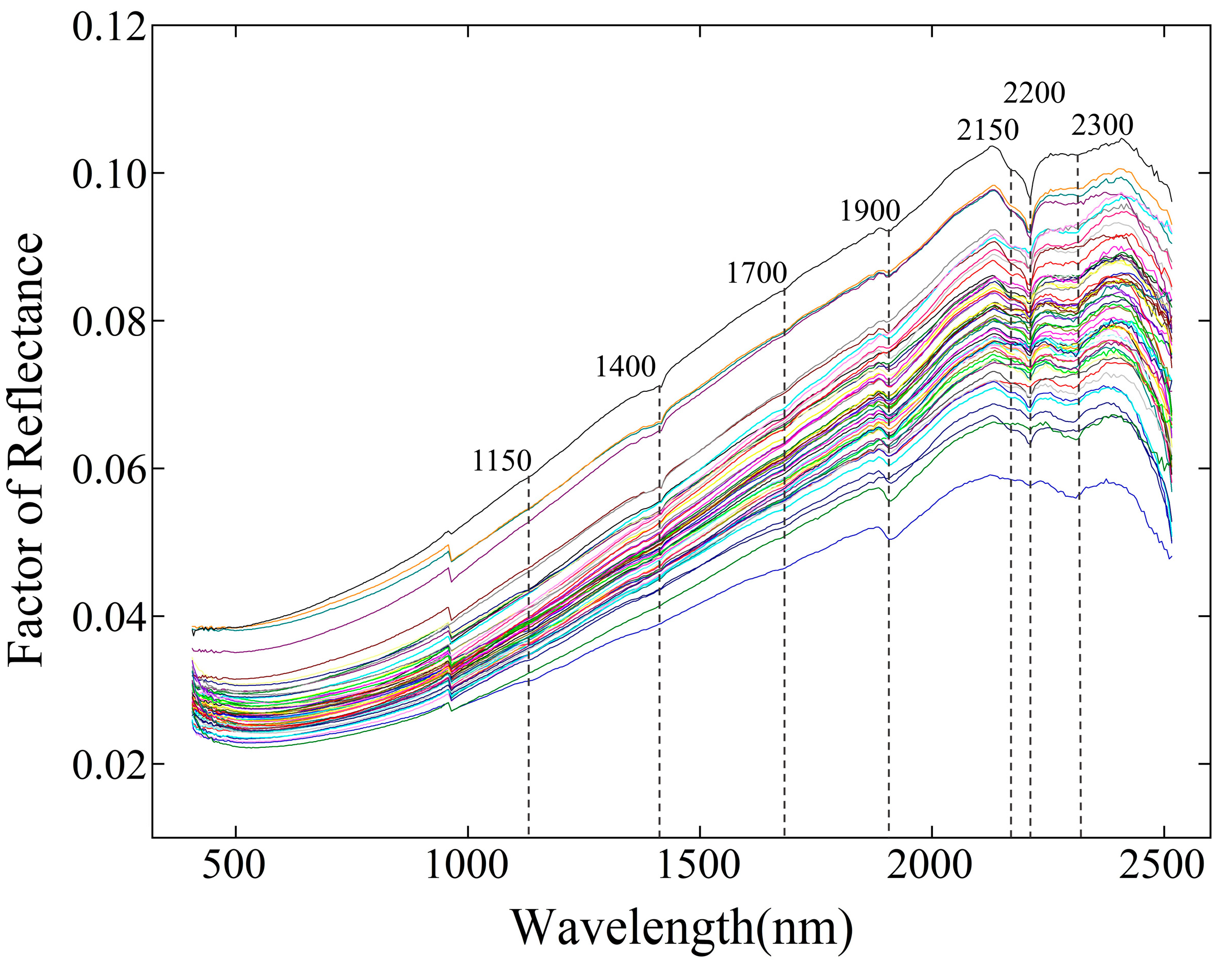
Figure 1. Research flow chart of the study.
Applsci 14 07920 g001
Figure 2. Pseudo-color images (817 nm, 661 nm, and 549 nm) of four coal samples and the measured values of quality indices. The samples are arranged from left to right by CV, from highest to lowest.
Applsci 14 07920 g002
Figure 3. Reflectance spectra and characteristic wavelengths obtained by averaging pixels in the region of interest from hyperspectral images of 61 coal samples. Each different colored curve represents each coal sample.
Applsci 14 07920 g003
Figure 4. Evolution of the noise level with wavelength evaluated based on spectra of all coal samples. Wavelengths with prominent noise spikes (>0.5%) have been excluded from further analysis.
Applsci 14 07920 g004
Figure 5. The spectral curves of (a) raw and preprocessed reflectance of all coal samples using (b) SG, (c) FD, and (d) MSC methods. The red curves indicate the mean spectra of all coal samples, and the gray shadows represent the spectra reflectance range.
Applsci 14 07920 g005
Figure 6. Results of characteristic wavelength extraction (marked by red square). The characteristic wavelengths of Ash, VM, MC, and CV were extracted by CARS. The characteristic wavelengths of FC were extracted by Boruta.
Applsci 14 07920 g006
Figure 7. Scatter plots of actual and predicted coal quality indices values obtained using the optimal LSSVR model based on the combined spectra-texture features. (a) Ash; (b) VM; (c) MC; (d) FC; and (e) CV.
Applsci 14 07920 g007
Figure 8. Contributions of the top ten significant variables by SHAP values in the coal quality indices optimal prediction models.
Applsci 14 07920 g008
Figure 9. Relative contribution of coal quality indices based on mean absolute SHAP values.
Applsci 14 07920 g009
Figure 10. Predictive distribution of coal quality indices by combined spectra-textual feature based on hyperspectral images. The four samples in each index correspond to the minimum, 25%, 75%, and maximum values in the dataset from left to right, respectively.
Applsci 14 07920 g010
Table 1. The characteristic wavelengths and corresponding groups or ions in coal proximate analysis based on hyperspectral images.
Featured Wavelength (nm)Groups or IonsReferences
1150Electron leaps in Fe 2 + -dominated metals[34]
1400Combined bands of H 2 O vibrations[34]
1700First overtones of CH 2 , CH 3 symmetric/asymmetric stretch.[34,35]
1900Combined bands of H 2 O vibrations[35]
2150Combination of aromatic C-H stretch and C-C stretch[35]
2200Combination Al-OH vibration[35,36]
2300Combination of CH 2 , CH 3 asymmetric stretch and bend[34,35]
Table 2. Statistical results of coal quality indices in calibration set and prediction set. The values in brackets indicate the number of samples in the calibration and prediction sets.
Coal Quality
Indices
Calibration Set (46)Prediction Set (15)
MinMaxMean S t d c MinMaxMean S t d p
Ash (%)17.7960.2436.4811.5122.5657.7034.168.06
MC (%)0.383.601.710.790.382.821.250.80
VM (%)9.5430.4920.006.5210.530.1821.975.77
FC (%)29.1254.3441.605.2531.4449.6343.233.81
CV ( MJ · kg 1 )11.6126.5519.963.8712.7525.0521.413.00
Table 3. PLSR modeling results based on the raw and different preprocessed spectra.
Coal Quality
Indices
SpectraPCsCalibration SetPrediction Set
R c 2 R M S E c R p 2 R M S E p
Ash (%)OR70.9572.2970.9302.242
SG70.9552.3330.9292.250
FD70.9950.7410.9711.723
MSC70.9851.3870.9721.342
VM (%)OR70.9641.2550.9301.378
SG70.9631.2720.9281.399
FD70.9960.4360.9481.030
MSC70.9820.9190.9690.801
MC (%)OR70.7550.4180.8030.300
SG70.7470.4240.8030.300
FD40.9610.1670.4730.438
MSC60.8060.3840.5810.366
FC (%)OR70.8951.6780.8121.618
SG70.8901.7240.8281.550
FD70.9820.6990.8501.534
MSC70.9421.2560.8591.426
CV (MJ/kg)OR160.9990.1160.9080.869
SG100.9810.5370.9640.545
FD70.9920.3430.9670.516
MSC130.9950.2830.9730.440
Table 4. Coal quality indices prediction results based on different wavelength selection methods with machine learning modeling.
Coal Quality IndicesMethodsNumber of WavelengthsModelingCalibration SetPrediction Set
R c 2 R M S E c R c v 2 R M S E c v R p 2 R M S E p R P D
Ash (%)SPA6PLSR0.8384.5020.7995.0240.7404.1762.032
RF0.9811.5340.9043.4620.9402.0084.225
BPNN0.9920.9950.8733.9880.8852.7853.047
LSSVR0.9781.6700.9672.0430.9421.9754.296
CARS65PLSR0.9452.6270.9243.0940.9322.1843.971
RF0.9851.3620.8724.0200.9212.3593.676
BPNN0.9920.9240.8194.7890.7544.1592.085
LSSVR0.9970.6360.9871.2780.9841.0578.202
Boruta12PLSR0.9761.8090.9711.9800.9511.4554.656
RF0.9881.2750.9193.3190.9631.2565.392
BPNN0.9741.8830.9043.6140.7863.0272.237
LSSVR0.9771.7900.9712.0040.9491.4814.572
iVISSA84PLSR0.9801.5920.9681.9980.9741.3646.400
RF0.9861.3060.9063.4350.9302.2283.919
BPNN0.9861.2910.8264.6660.6994.6261.887
LSSVR0.9921.0080.9801.5710.9711.4256.128
VM (%)SPA10PLSR0.9361.7230.9052.0960.8881.3883.094
RF0.9751.0680.8122.9580.8471.6232.647
BPNN0.9511.5020.8882.2760.9091.2493.438
LSSVR0.9651.2740.9351.7440.9450.9774.398
CARS26PLSR0.9052.0560.8642.4620.8291.8962.504
RF0.9541.4350.6823.7660.8241.9222.470
BPNN0.9830.8550.8682.4300.7822.1402.218
LSSVR0.9910.6470.9771.0140.9710.7876.030
Boruta11PLSR0.8013.0120.7723.2270.9231.2883.725
RF0.9551.4340.8072.9700.9820.6217.729
BPNN0.9671.2240.9002.1420.8561.7602.725
LSSVR0.8932.2130.8672.4690.9670.8465.669
iVISSA136PLSR0.9121.9560.8722.3660.8871.7383.076
RF0.9381.6430.5734.3230.7902.3682.257
BPNN0.9850.7400.8122.8700.7072.7971.911
LSSVR0.9890.7010.9411.6070.9291.3733.894
MC (%)SPA4PLSR0.6560.4910.6080.5250.7040.3591.902
RF0.8320.3430.3980.6510.5840.4251.605
BPNN0.8780.2930.7310.4350.7700.3132.178
LSSVR0.6950.4630.6350.5070.7710.3142.174
CARS25PLSR0.6720.4960.5600.5740.6010.3731.640
RF0.7810.4050.2760.737−0.2550.6620.924
BPNN0.8440.3410.5860.5570.5390.4011.524
LSSVR0.9650.1630.9040.2680.7720.2822.165
Boruta8PLSR0.5660.5460.5100.5800.6610.4301.778
RF0.7540.4110.5160.5770.7840.3432.225
BPNN0.8160.3540.4130.6350.4730.5351.426
LSSVR0.6430.4950.5460.5580.7140.3951.934
iVISSA91PLSR0.7170.4600.6410.5180.3630.4511.297
RF0.7780.4070.4380.6480.3940.4401.329
BPNN0.8210.3660.6480.5130.0830.5411.081
LSSVR0.7710.4140.6570.5060.4490.4191.395
FC (%)SPA6PLSR0.8022.3080.7312.6940.8451.5392.631
RF0.9710.8770.7892.3850.8301.6142.507
BPNN0.8641.9130.7272.7150.2363.4181.184
LSSVR0.8771.8180.8102.2620.7941.7742.283
CARS35PLSR0.8981.7520.8292.2690.1211.8571.104
RF0.9591.1080.7152.9290.2081.7631.163
BPNN0.8961.7640.7742.608−3.7904.3330.473
LSSVR0.9810.7550.9251.5030.6491.1721.748
Boruta14PLSR0.8881.7890.8462.0990.8651.1792.813
RF0.9660.9790.7672.5820.9090.9643.439
BPNN0.8012.3830.6033.3750.7171.7031.947
LSSVR0.8941.7430.8452.1050.8841.0933.033
iVISSA104PLSR0.8192.2310.7202.7760.8171.5392.422
RF0.9371.3120.5333.5840.8161.5432.414
BPNN0.8631.9380.6223.2240.0423.5231.058
LSSVR0.8991.6650.7992.3530.8781.2562.965
CV (MJ/kg)SPA8PLSR0.8861.3040.8551.4710.8970.9383.232
RF0.9730.6370.9350.9830.9350.7454.066
BPNN0.9590.7860.9191.0960.9330.7564.007
LSSVR0.9830.5100.9730.6300.9730.4806.315
CARS48PLSR0.9530.8420.9231.0740.9470.6464.490
RF0.9810.5350.8671.4130.9110.8353.474
BPNN0.9880.4280.8011.7320.6531.6511.757
LSSVR0.9950.2670.9810.5350.9910.26011.156
Boruta14PLSR0.9740.6360.9640.7500.9560.5504.958
RF0.9750.6190.8861.3340.9370.6634.113
BPNN0.9620.7740.9191.1270.9090.7933.439
LSSVR0.9750.6260.9640.7550.9620.5125.321
iVISSA122PLSR0.8741.3570.8261.5960.7681.4252.148
RF0.9161.1090.4232.9040.4472.2001.392
BPNN0.9880.3970.6832.1520.3672.3541.301
LSSVR0.9870.4410.9490.8600.9450.6964.401
Table 5. Coal quality indices prediction model results based on texture features and combined spectra-texture features. Combination = combination of spectra and texture features.
Coal Quality IndicesFeature
Data
Number of FeaturesCalibration SetPrediction Set
R c 2 R M S E c R c v 2 R M S E c v R p 2 R M S E p R P D
Ash (%)HS500.9861.3310.8524.3260.7833.9012.223
GLEM440.9801.6610.5807.5910.6443.5691.736
Gabor370.9921.0270.9472.6010.8113.4522.379
Combined710.9980.4760.9861.3410.9930.65912.217
VM (%)HS410.9800.8800.8222.6230.8462.3712.634
GLEM440.9910.6160.8562.4140.8921.9993.149
Gabor490.9940.5090.9231.8780.9271.1353.842
Combined430.9990.2300.9940.4970.9890.5839.904
MC (%)HS370.9630.1520.7300.4120.5830.4861.603
GLEM180.8560.2990.6380.4760.5020.5631.467
Gabor330.9910.0750.9230.2180.9570.1744.991
Combined560.9950.0550.9610.1540.9790.1127.159
FC (%)HS410.8651.9600.4723.8750.5142.2591.485
GLEM620.9670.9750.3574.315−0.9322.8470.745
Gabor220.9421.3110.7362.794−0.9042.2610.750
Combined780.9890.5530.9231.4380.9480.8384.544
CV (MJ/kg)HS370.9790.5670.8741.3910.5651.4811.570
GLEM490.9700.6650.5952.4520.6461.7711.741
Gabor560.9920.3650.8641.4870.6190.9941.676
Combined450.9980.1570.9890.4090.9940.21713.849
Disclaimer/Publisher’s Note: The statements, opinions and data contained in all publications are solely those of the individual author(s) and contributor(s) and not of MDPI and/or the editor(s). MDPI and/or the editor(s) disclaim responsibility for any injury to people or property resulting from any ideas, methods, instructions or products referred to in the content.

