EGS-YOLO: A Fast and Reliable Safety Helmet Detection Method Modified Based on YOLOv7

Abstract

Wearing safety helmets at construction sites is a major measure to prevent safety accidents, so it is essential to supervise and ensure that workers wear safety helmets. This requires a high degree of real-time performance. We improved the network structure based on YOLOv7. To enhance real-time performance, we introduced GhostModule after comparing various modules to create a new efficient structure that generates more feature mappings with fewer linear operations. SE blocks were introduced after comparing several attention mechanisms to highlight important information in the image. The EIOU loss function was introduced to speed up the convergence of the model. Eventually, we constructed the efficient model EGS-YOLO. EGS-YOLO achieves a mAP of 91.1%, 0.2% higher than YOLOv7, and the inference time is 13.3% faster than YOLOv7 at 3.9 ms (RTX 3090). The parameters and computational complexity are reduced by 37.3% and 33.8%, respectively. The enhanced real-time performance while maintaining the original high precision can meet actual detection requirements.

1. Introduction

Building construction, road construction, and other types of construction are high-risk operations. During construction activities, improper operations and construction personnel failing to follow prescribed measures can cause damage to their life and health. Among these risks, improper wearing of protective devices is a major cause of serious consequences. According to statistics, there were 689 municipal engineering production safety accidents in China in 2020, including 83 incidents of physical strikes. These statistics indicate that it is essential to take safety protection measures at construction sites.

Head injuries during construction are extremely dangerous. Helmets can absorb external impact forces and prevent object penetration, making them essential tools for reducing the incidence of such injuries. However, according to a survey by the Bureau of Labor Statistics, 84 percent of workers who suffered head injuries were not wearing helmets [1]. Therefore, monitoring the use of helmets by construction workers is crucial.

Manual monitoring is costly, time-consuming, and inefficient. In contrast, automatic detection and supervision, facilitated by computer vision, the Internet, and other technologies, have emerged as new developmental trends. This approach offers both cost savings and significantly increased security. Research into construction site security protection, closely integrated with deep learning technology, is gradually becoming a hotspot among scholars. This research provides a new model for production safety management and can offer technical support and references for future smart construction sites, intelligent manufacturing, and other fields.

In previous studies, safety helmet detection primarily involved traditional methods and deep learning-based approaches. Initially, Kelm et al. [2] proposed the employment of RFID (Radio Frequency Identification) to check workers’ compliance with safety wear. However, RFID is limited in scope, as it can only confirm the helmet’s proximity to the worker, not whether it is being worn correctly. Santiago et al. [3] put forward a cyber-physical system (CPS) to detect workers wearing PPE (personal protective equipment) in real-time, but this system could not determine whether workers were wearing helmets correctly. Dong et al. [4] utilized a positioning system for virtual building technology where a pressure sensor in the helmet recorded relevant information and relayed it via Bluetooth. However, this method was ineffective over long distances. Sun X et al. [5] employed a visual background difference algorithm for worker identification and used principal component analysis for feature dimensionality reduction. They ultimately used the Bayesian optimization SVM (Support Vector Machine) model to identify hard hats, but the accuracy was not high. Traditional methods for safety helmet detection have low accuracy, poor generalization, and low efficiency. Consequently, deep learning-based object detection techniques are now the preferred approach.

Qi Fang et al. [6] implemented helmet detection using Faster R-CNN for targets in the far field and scenes with various construction site backgrounds, achieving excellent detection results on the collected dataset. Although the Faster R-CNN model has higher detection accuracy, it is poor in real-time and has a large model size. Zhao et al. [7] addressed the problem of low helmet detection accuracy; they improved YOLOv5 by increasing the detection head, feature fusion, and attention mechanism, which enhanced the model’s detection accuracy in complex backgrounds, and the average accuracy was improved by 2.6%. However, the inference time of the model is not satisfactory enough, and there is a large room for improvement. Hayat et al. [8] conducted extensive experimental research on helmet detection systems and found that YOLOv5X performs excellently in low-light conditions with high precision. However, the YOLOv5X model is large, and its inference time requires further investigation. Z. Li et al. [9] proposed a safe helmet detection algorithm based on YOLOv5s. The approach employed a hierarchical sample selection mechanism and a density-based post-processing algorithm, significantly enhancing detection accuracy. Their method improved F1 scores by 12.47% at a threshold of 0.1. However, the speed of model detection was largely overlooked. Li et al. [10] introduced a model based on Faster R-CNN-LSTM to address the accuracy issues due to an insufficient spatial and temporal feature mining in the detection process. The improved model fuses temporal and spatial features, greatly enhancing accuracy. However, the model has a large number of parameters, and the inference time needs further improvement. Fu et al. [11] proposed the YOLOv8n-FADS helmet detection algorithm, which improves the detection head, enhancing the model’s ability to perceive complex patterns and handle occlusions effectively. Although the parameters and accuracy of the model have been improved, the overall accuracy is not high, and the inference time needs further improvement. Barlybayev et al. [12] used YOLOv8 to detect PPE. It was concluded that YOLOv8x and YOLOv8l performed well on PPE detection. However, the detection accuracy in complex backgrounds needs to be further improved, and the number of parameters and inference time of the models also need to be improved. He et al. [13] proposed a lightweight helmet detection algorithm called YOLO-M3C, which uses MobileNetV3 instead of the YOLOv5s backbone network and introduces the CA attention mechanism and knowledge distillation. The model size and detection speed are effectively improved. However, the accuracy of the method only reaches 82.2%, which is not very reliable. Xu et al. [14] proposed MCX-YOLOv5 to address the problem of low detection accuracy caused by the small size of the helmet. Several methods, including a coordinate space attention module, a multi-scale asymmetric convolutional downsampling module, and a lightweight decoupling head, were used. Through several experiments, the accuracy of the method is improved by 2.7% compared to YOLOv5. However, the inference time of the algorithm still has a large room for improvement.

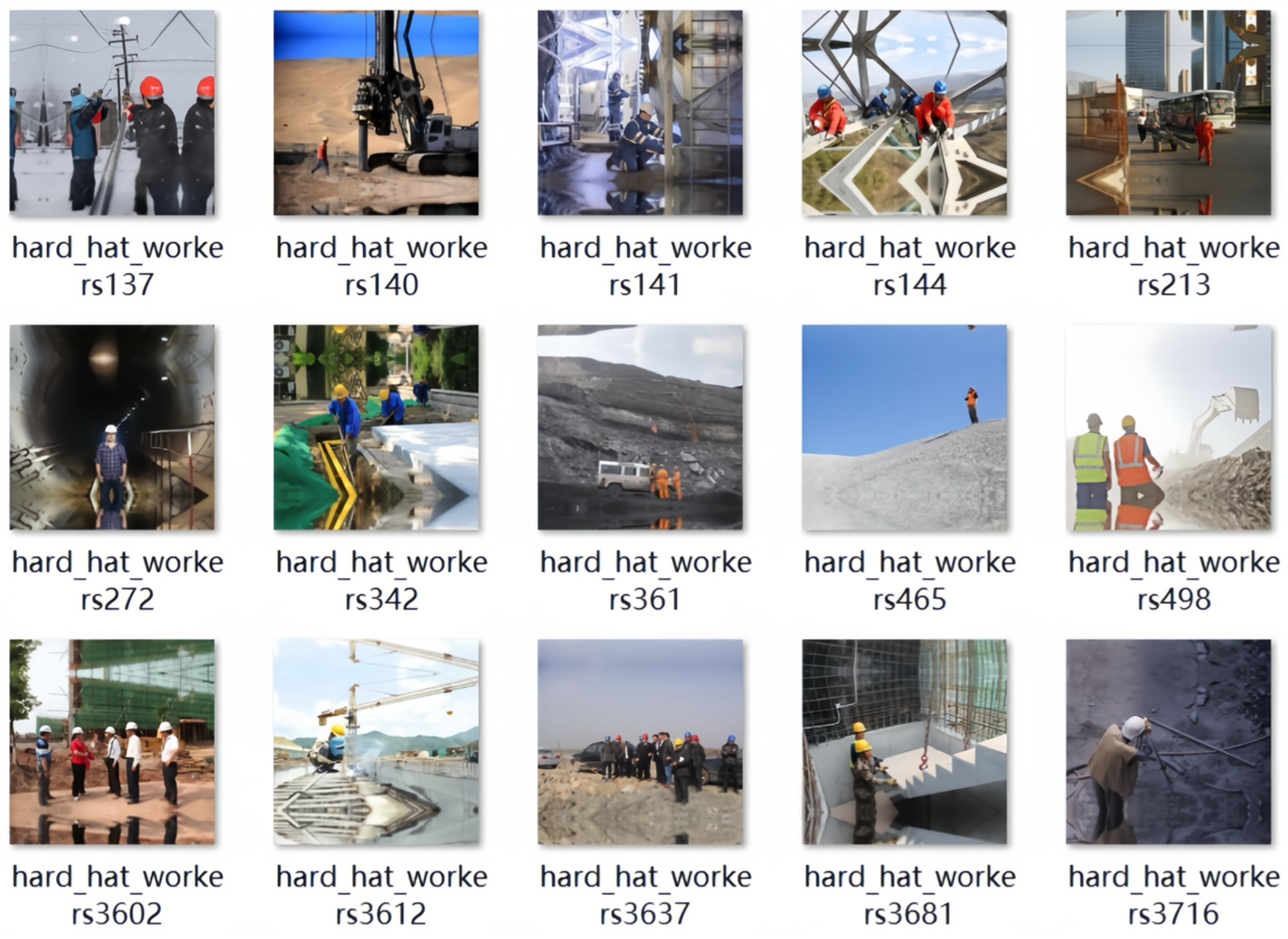
In the aforementioned studies, most of them focus on how to improve the detection accuracy of safety helmets, ignoring the attention to the inference time or the number of parameters. Enhancing inference time and reducing parameters will help the models to be more practical. Therefore, it is necessary to increase inference speed and decrease parameters while maintaining accuracy. Based on this, we propose EGS-YOLO. EGS represents EIOU, GhostModule, SE, respectively. The real-time performance is enhanced while maintaining high detection accuracy and achieving a certain degree of being lightweight. The method is validated by using the SHEL5K [15] dataset. In our study, in order to speed up the inference of the model and enable the model to fully process useful information in complex contexts with low-cost operations, we improved YOLOv7 using three approaches: GhostModule, SE (Squeeze and Excitation), and EIOU (Efficient Intersection over Union). This paper completes the following:

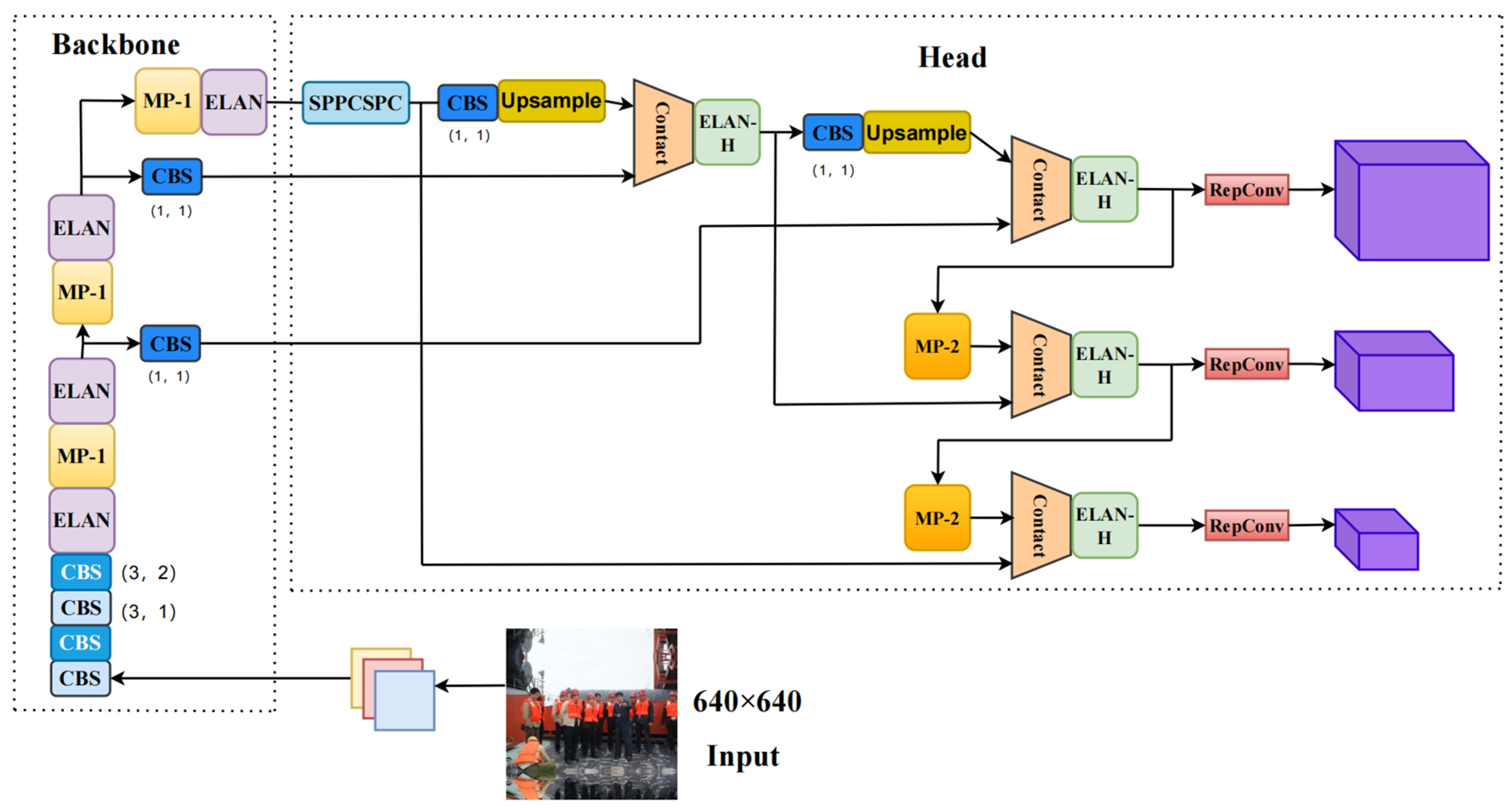
• Based on YOLOv7 [16], to increase the model’s inference speed and decrease parameters, part of the CBS modules are replaced with GhostModule to compose efficient structures. After comparing it with several other lightweight modules, GhostModule was selected. Reducing computing costs.
• To enhance the feature extraction performance of the model in complex contexts, the SE attention mechanism is adopted into the model. This allows the model to focus on worthwhile information in the image without compromising inference speed. After comparing it with several other attention mechanisms, SE was selected.
• To accelerate the model’s convergence, the EIOU loss function is introduced. This helps the model focus on the difference between the width and height of the object in the image rather than the aspect ratio.

2. YOLOv7 Object Detection Algorithm

2.1. Object Detection Algorithm

Object detection is commonly applied in a broad range of industries, such as automated driving, medicine, and industrial inspection. Object detection can be summarized in two points: positioning and classification. Deep learning-based object detection techniques can typically be categorized into two groups: two-stage object detection algorithms and one-stage object detection algorithms. The two-stage detection algorithm first performs feature extraction before classifying the image. Typical algorithms include R-CNN [17], Fast R-CNN [18], and Faster R-CNN [19]. Although two-stage object detection algorithms perform well in terms of accuracy, they have the disadvantage of poor real-time performance.

One-stage detection means that only one feature extraction is needed to achieve object detection. Typical algorithms are SSD [20], YOLO [21] series, and so on. The YOLO series algorithms can input an image and directly output the final result, including the name of the detected object and its score. In contrast to the two-stage object detection algorithms, YOLO performs the task of detecting and classifying objects with just one network. The most prominent feature of the YOLO series is its excellent real-time performance. Meanwhile, the algorithms are increasing in accuracy with each generation. YOLOv7 is one of the most advanced detection algorithms available, with superior performance in detection accuracy and speed. Hence, we further investigate based on the foundation of YOLOv7.

2.2. YOLOv7 Structure

YOLOv7 was released in October 2022, and its performance is at the forefront of the field. It surpasses previous YOLO series algorithms in both speed and accuracy. YOLOv7 was improved based on YOLOv5, with additional convolutional layers added to the network to effectively handle complex scenes and targets of various scales, further enhancing detection precision.

The overall structure of YOLOv7 consists of three main components: the input, the backbone, and the detection head, as illustrated in Figure 1.

In the backbone network, the input 640 × 640 size image is scaled down to a 10 × 10 feature map after multiple convolution and subsampling processes. At the detection head, the shallow backbone features are fused with the deeper features by channel stitching. Next, three layers of max-pooling and convolution operations are performed on the 80 × 80 feature maps, producing four layers of feature maps of different sizes. Finally, the prediction results are obtained through RepConv.

The CBS (Convolution Batch Normalization Silu) structure is composed of a Silu activation function, a Batch Normalization (BN) layer, and a convolution layer. The Silu function is a special case of the Swish function, as can be seen from Equations (1) and (2).

$$silu\left(x\right)=x•sigomid\left(x\right)$$

(1)

$$swish\left(x\right)=x•sigomid\left(\beta x\right)$$

(2)

CBS has three different types, each featuring varying convolution kernels and stride lengths. It serves purposes such as changing channel numbers, feature extraction, and subsampling. The structure of CBS is presented in Figure 2.

The ELAN (Efficient Layer Adaptive Network) module enables better feature learning by manipulating the gradient paths. This is an efficient and robust network structure. The structure of ELAN is visible in Figure 3.

The ELAN-H (Efficient Layer Adaptive Network-H) structure shares structural and functional similarities with ELAN. The difference is that ELAN-H selects a different amount of output superposition in the second branching. The structure of ELAN-H is presented in Figure 4.

The MP (max-pooling) is charged with subsampling. The final subsampling result is generated by summing the outputs of the two branches. The structure of MP is visible in Figure 5.

The SPPCSPC (Spatial Pyramid Pooling Concurrent Spatial Pyramid Convolution) structure is formed by two parts. It expands the receptive field through a max-pooling operation, allowing the algorithm to process images of various sizes. The structure of SPPCSPC is presented in Figure 6.

3. Proposed Method EGS-YOLO

To construct a helmet-wearing detection model with superior comprehensive performance, we integrate GhostModule, SE, and EIOU into the network structure of YOLOv7 to achieve high real-time performance while maintaining high accuracy.

3.1. GhostModule

To achieve high real-time performance in helmet wear detection, a preferable approach involves lightening the model. A better real-time and lighter-weight model will facilitate deployment into embedded devices. As convolutional neural networks continue to progress, lightweight convolutional neural networks are becoming highly favored, and this trend will likely continue in the future.

A main approach to creating lightweight neural networks is designing compact models, and many such models have emerged in recent years. The idea behind MobileNetv1 [22] is depthwise separable convolutions, a lightweight architecture. MobileNetv2 [23] introduces linear bottlenecks and inverse residuals based on the previous generation, enhancing the network’s representation ability. MobileNetv3 [24] incorporates the SE module, updates the activation function, and achieves better performance. MBConv [25] is an inverse residual structure that combines depthwise separable convolutions and attention mechanisms, characterized by inverted linearity. DSConv (depthwise separable convolution) [26] is a flexible, lightweight convolution operator that replaces single-precision operations with low-cost integer operations while maintaining performance. PConv (Partial Convolution) [27] can reduce redundant calculations and storage access, making the model more effective at extracting spatial features and maintaining performance while remaining lightweight. However, none of the above methods makes adequate use of feature mapping, and they do not handle redundant feature maps very well. GhostModule is an effective way to address these issues at a lower operational cost and is especially suitable for scenes with complex image backgrounds.

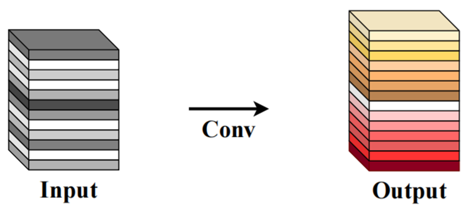
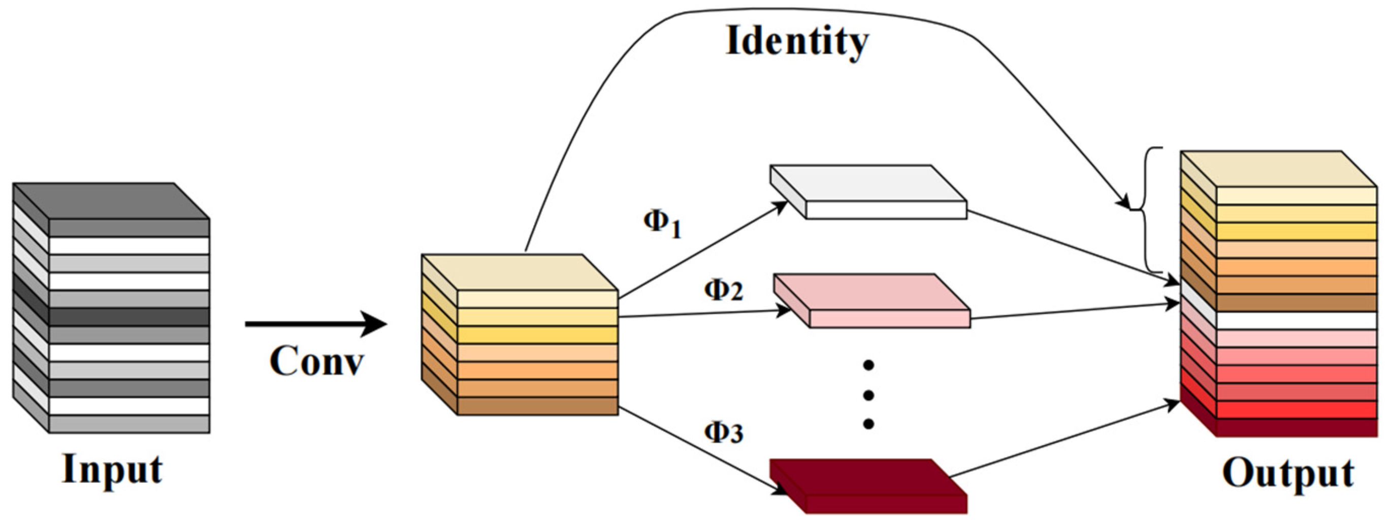
Han Kai et al. proposed GhostModule, a module capable of generating more feature maps from low-cost operations. Based on a set of inherent feature maps, a series of low-cost linear transformations are used to generate many feature maps that can reveal inherent feature information [28]. Compared with normal convolution, GhostModule requires less computational complexity and fewer parameters while maintaining similar performance. After some experimentation, GhostModule was the most suitable choice in this study. GhostModule can effectively deal with the redundancy of feature maps. Ordinary convolution and GhostModule are shown in Figure 7 and Figure 8, respectively. In Figure 8, the GhostModule is divided into three parts. The first part is a normal convolution operation, the second part is a grouped convolution operation, and the third part is Identity, which is the sum of the number of channels in the first and second parts.

GhostModule can be divided into two steps: The first part performs ordinary convolution and limits the quantity of convolution; the second part consists of some low-cost linear transformations that use the inherent feature mappings to yield more feature mappings. The feature maps generated from the two sections are then stitched together to produce a new output. This procedure enhances real-time performance and decreases the model’s parameters and computational complexity with minimal loss of precision. The ratio of computational and parametric quantities for ordinary convolution is shown in Equation (3).

In Equation (3), $c$ is the channel of the input, $n$ is the number of channels, $h^{\prime }$ and $w^{\prime }$ are, respectively, the width and height of the output data, $k\cdot k$ is the kernel size of the convolution filter, $d\cdot d$ represents the kernel size of each linear operation. The ratio of the amount of calculation and the number of parameters of GhostModule is shown in Equation (4).

In Equation (4), $s$ directly impacts the ratio of computational and parametric quantities. The more feature maps produced in that output, the better the acceleration. Introducing GhostModule into the model allows the model to utilize the correlation and redundancy between feature mappings in a better way, generating many more feature maps, decreasing the parameters and calculations in the model, and enhancing speed.

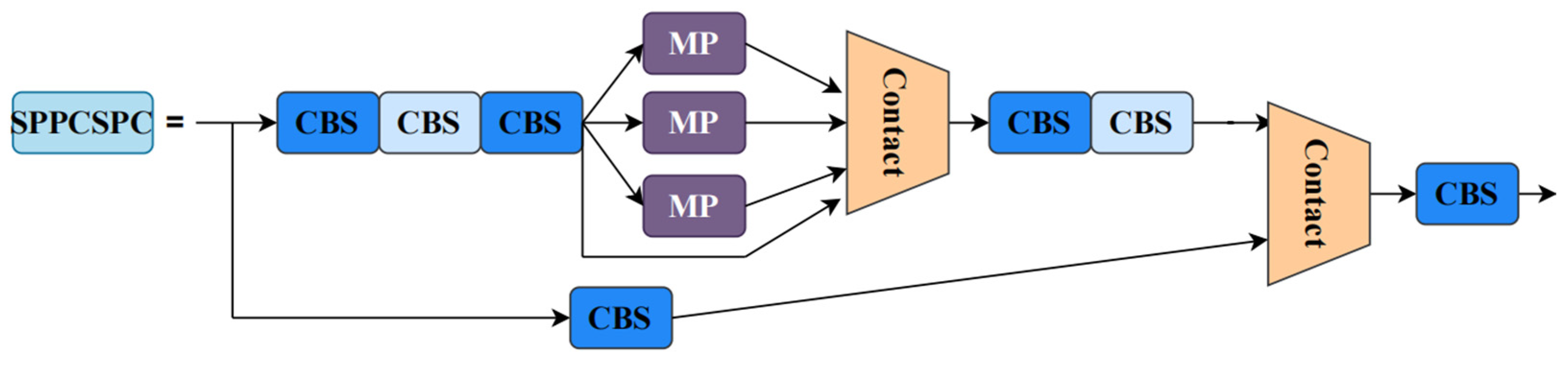
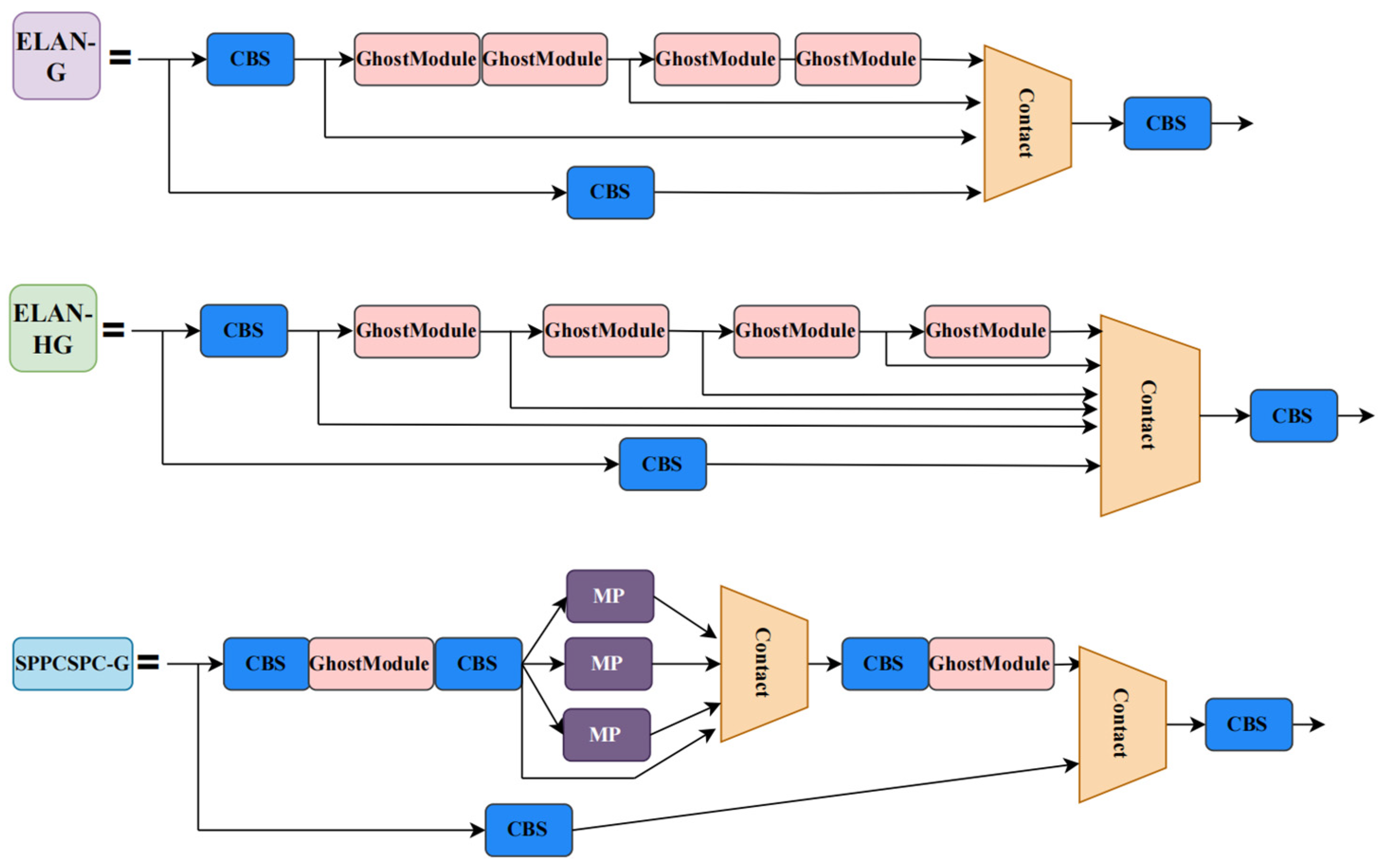
In YOLOv7, the major function of a 3 × 3 convolution with a step size of 1 is to perform feature extraction; these convolutions are computationally intensive. We use the low-computation GhostModule instead of these convolutions. In this part, the CBS modules that conduct feature extraction operations in ELAN, ELAN-H, and SPPCSPC are replaced by GhostModule, that is, replacing the CBS module with a 3 × 3 kernel and a stride of 1 in these structures with the GhostModule. The new structures ELAN-G, ELAN-HG, and SPPCPSC-G are, respectively, presented in Figure 9. The enhanced structures can generate feature maps that reveal intrinsic feature information through a series of cost-effective operations. However, it also affects the model’s feature extraction capability and convergence speed, resulting in a loss of accuracy. Measures will be taken next to resolve this issue.

$$\begin{array}{lll}{r}_s& =& {\displaystyle \frac{n\cdot h^{\prime }\cdot w^{\prime }\cdot c\cdot k\cdot k}{\frac{n}{s}{h}^{\prime }\cdot w^{\prime }\cdot c\cdot k\cdot k+\left(s-1\right)\cdot \frac{n}{s}\cdot h^{\prime }\cdot w^{\prime }\cdot d\cdot d}}\\ & =& {\displaystyle \frac{c\cdot k\cdot k}{\frac{1}{s}\cdot c\cdot k\cdot k+\frac{s-1}{s}\cdot d\cdot d}}\approx {\displaystyle \frac{s\cdot c}{s+c-1}}\approx s\end{array}$$

(3)

$$r_c={\displaystyle \frac{n\cdot c\cdot k\cdot k}{\frac{n}{s}\cdot c\cdot k\cdot k+\left(s-1\right)\cdot \frac{n}{s}\cdot d\cdot d}}\approx {\displaystyle \frac{s\cdot c}{s+c-1}}\approx s$$

(4)

3.2. SE (Squeeze and Excitation Block)

As for limited computational power, the attention mechanism can distribute computational power to the more important parts of the task. Attention mechanisms are widely used in deep learning to enhance the performance of models [29]. Currently, attention mechanisms are categorized into three types. The squeeze excitation network (SENet) [30] is a typical representative of channel attention. The second type is the spatial attention mechanism, with SAM [31] as a typical example. The third type is the mixed frequency domain mechanism, with CBAM [32] as its representative. SE is able to reduce the problem of vanishing gradients by re-weighting the channel features. To speed up the model’s inference time and lighten the model, we introduced GhostModule. However, this weakened the model’s feature extraction capability, leading to a loss in accuracy. To address this, we incorporated attention mechanisms.

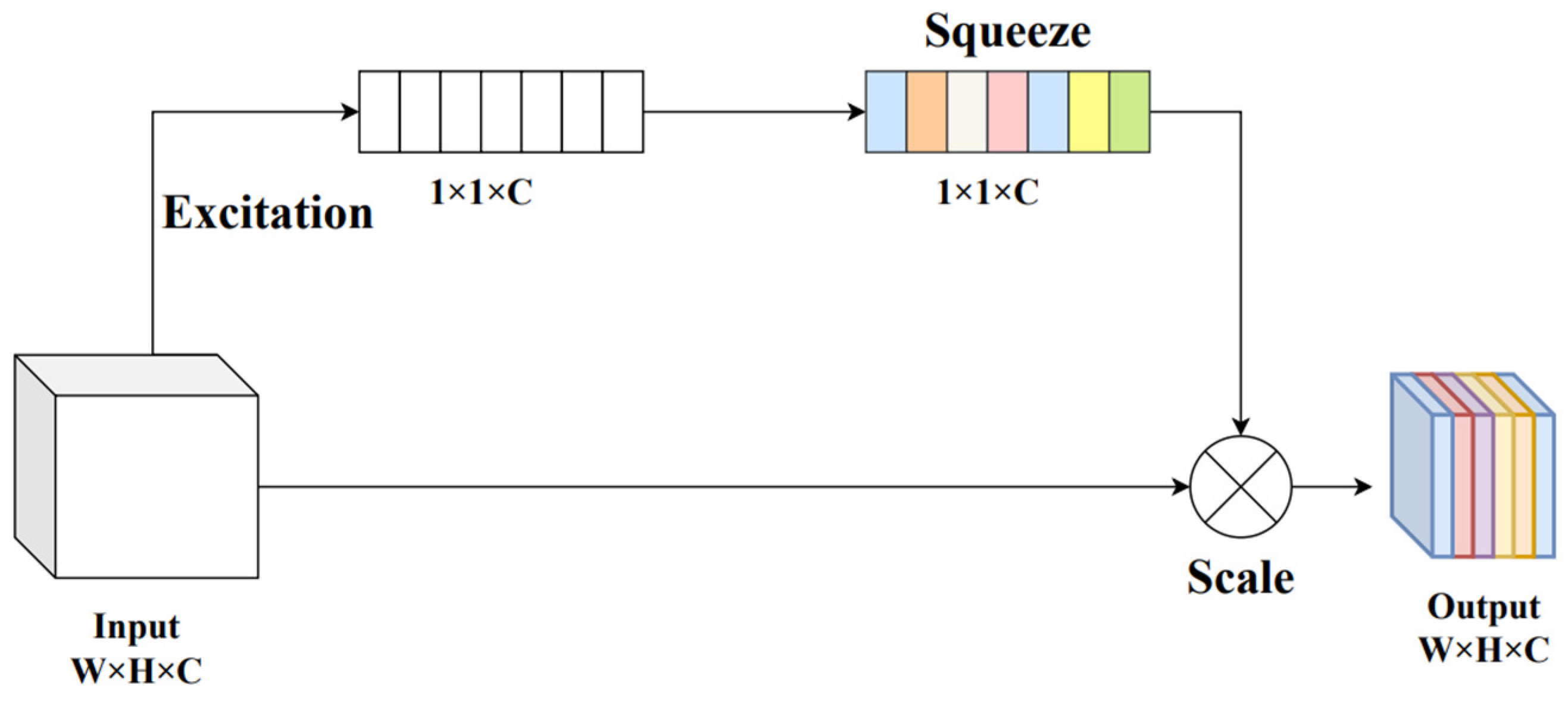
The SE (Squeeze-and-Excitation) module can mitigate the problem of accuracy loss due to the different significance attributed to various channels. This unit adaptively recalibrates the channel feature response by explicitly modeling the interdependencies between channels. The goal is to improve the quality of the representations produced by the network by highlighting valuable parts and suppressing less meaningful information. SE allows networks to use overall information to selectively emphasize significant features. The context of construction sites is usually complex and diverse, causing many interferences and difficulties in helmet detection. SE suppresses insignificant information in the image, making it effective for tasks like helmet detection with mixed backgrounds. And we have experimented with a variety of attention mechanisms to conclude that SE is the most appropriate choice. SE is more lightweight and has almost no effect on the parameters. The structure of SE is visible in Figure 10; the image input is first subjected to a Squeeze-and-Excitation operation, followed by a scale operation to generate the final feature map.

An SE block is equivalent to a calculation unit. The feature map $U$ is generated by passing the input $X$ through the transformation operation, as shown in Equation (5). The output is expressed as $U=\left[u_1,u_2,\cdots ,u_c\right]$.

$$u_c=v_c\ast X=\sum _{s=1}^{c^{\prime }}{v}_c^s\ast x^s$$

(5)

$v_c$ indicates the 2D spatial kernel of a single channel, which acts on the correspondent channel of $X$. There are two key steps in the SE block: the compression operation and the excitation operation.

The compression procedure is essentially a process of global average pooling. It compresses the global spatial information into the channel descriptor. The channel statistics are generated by using global average pooling, resulting in a feature map as a 1*1*C vector, where a numerical value represents each channel. This operation is shown in Equation (6).

$$z_c=F_{sq}(u_c)={\displaystyle \frac{1}{H\times W}}\sum _{i=1}^H\sum _{j=1}^W{u}_c\left(i,j\right)$$

(6)

Here, $H$ and $W$ are, respectively, the height and width of the feature map.

The second step is the excitation operation, which obtains channel-related reliance relationships using the information aggregated during the compression operation. This is done through two fully connected layers, as shown in Equation (7).

$$s=F_{ex}\left(z,W\right)=\sigma \left(g\left(z,W\right)\right)=\sigma \left(W_2\delta \left(W_{1}z\right)\right)$$

(7)

$W$ is the weight, through which the required weight information is generated, and the value of $W$ is produced by learning. $\delta$ is the ReLU function.

The final output of the block is to weight the generated weight $s$ to the feature map $U$, as shown in Equation (8).

$${\tilde{x}}_c=F_{scale}\left(u_c,s_c\right)=s_c{u}_c$$

(8)

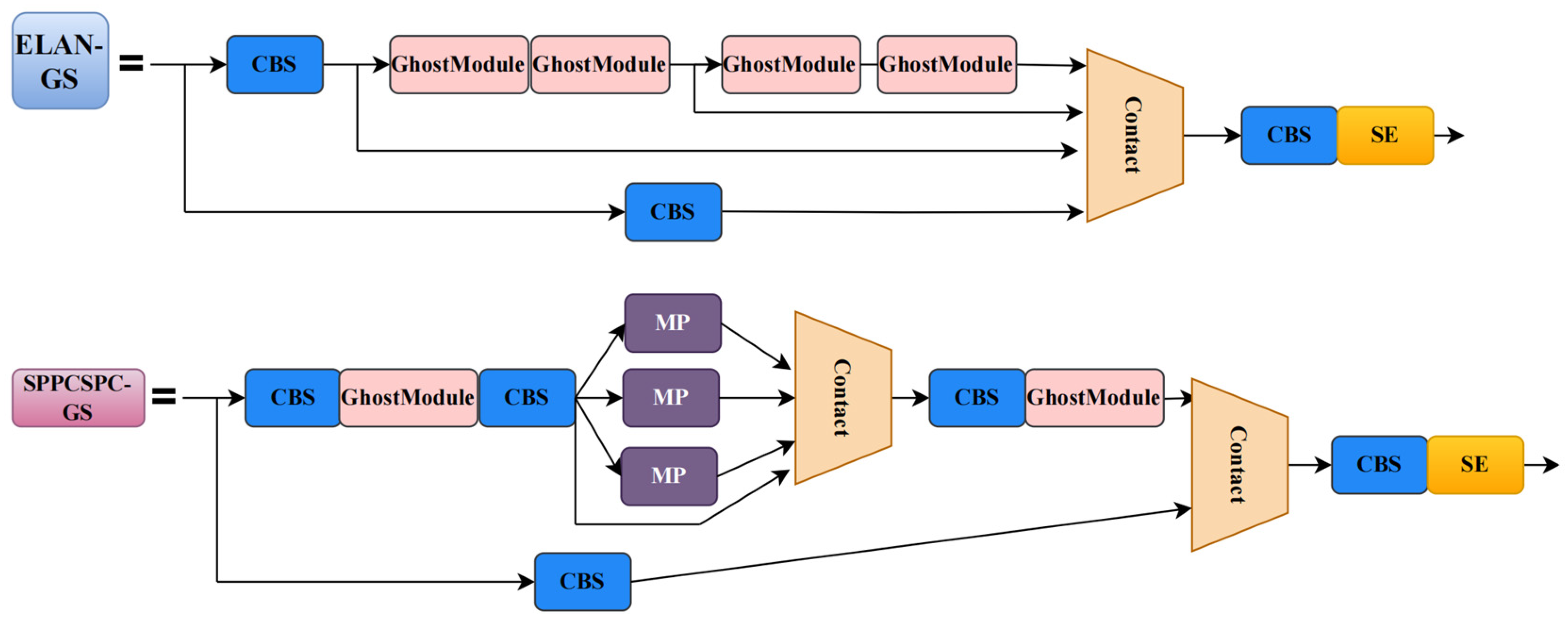
$\tilde{x}=[{\tilde{x}}_1,{\tilde{x}}_2,\cdots ,{\tilde{x}}_{\mathrm{c}}]$, $F_{scale}\left(u_c,s_c\right)$ represents the channal-by-channel multiplication between the scalar $s_c$ and the feature map $u_cϵR^{H\times W}$. The key information in the image is amplified once again after the squeeze and excitation operations, effectively reducing the interference from complex backgrounds in helmet wear detection. Building on the introduction of the GhostModule in the previous section, we have embedded SE into the structure ELAN-G and SPPCSPC-G. The SE together with the GhostModule compose the new efficient structures ELAN-GS and SPPCSPC-GS, as presented in Figure 11. We have embedded a total of four SE blocks into the model, specifically positioned as shown in Figure 12, labeled ELAN-GS and SPPCSPC-GS. 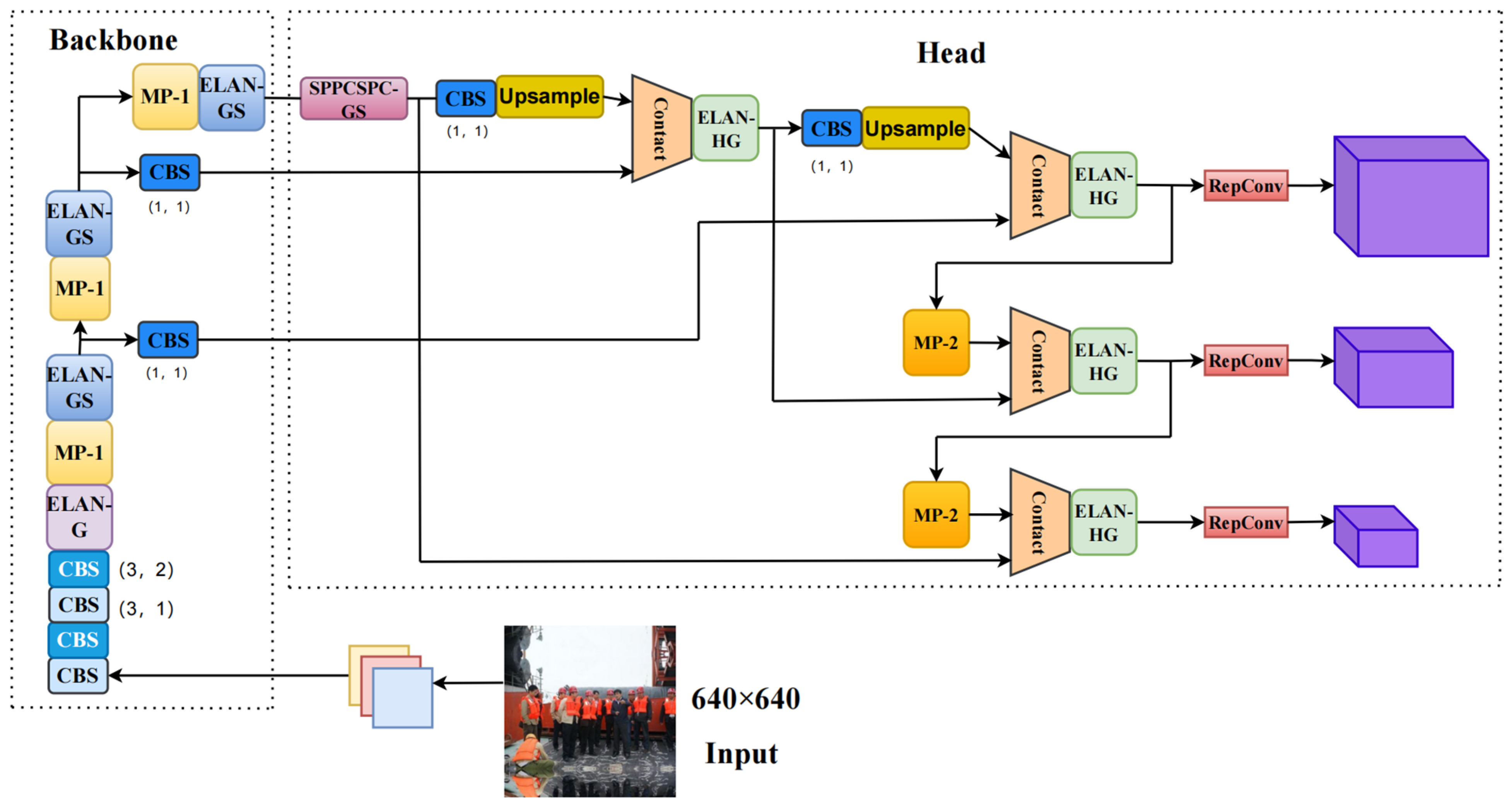Figure 12 shows the model structure of EGS-YOLO, we improve on the structures ELAN, ELAN-H, and SPPCSPC in YOLOv7 by constructing ELAN-G, ELAN-HG, ELAN-GS, and SPPCSPC-GS.

3.3. EIOU Loss

The loss function is crucial in judging the difference between the forecast and the true value. The Intersection over Union (IOU) ratio is a widely used index to indicate the precision of prediction boxes in object detection tasks. Many loss functions based on IOU have been proposed to optimize detection.

DIOU [33] loss makes it more robust by considering the distance and area of overlap between the target and the forecast. CIOU (Complete Intersection over Union) adds two new losses, a detection box scale, and an aspect to make the target box regression more stable. The idea of EIOU [34] is to separate the impact factors of the aspect ratio of the predicted box and the real box and to calculate the length and width of the predicted box and the real box separately.

The original loss function of YOLOv7 is CIOU, which adequately takes into account the overlap area, center-of-mass distance, and aspect ratio between the predicted and real boxes. The CIOU contains three main components: loss of target box and prediction box position, classification loss, and loss of target confidence. The CIOU is presented in Equation (9).

$$L_{CIOU}=1-IOU+{\displaystyle \frac{{\rho }^2\left(b,b^{gt}\right)}{c^2}}+\alpha v$$

(9)

$$\alpha ={\displaystyle \frac{v}{\left(1-IOU\right)+v}}$$

(10)

$$v={\displaystyle \frac{4}{{\pi }^2}}{\left(\left(\mathit{arctan}{\displaystyle \frac{w^{gt}}{h^{gt}}}\right)-\mathit{arctan}{\displaystyle \frac{w}{h}}\right)}^2$$

(11)

The ratio of the intersection and concatenation between two bounding boxes is defined as IOU. The centroids of the prediction and real frames are represented by $b$ and $b^{gt}$, respectively. The Euclidean distance between the center of mass in the prediction box and the center of mass in the real box is designated by $\rho \left(b,b^{gt}\right)$.

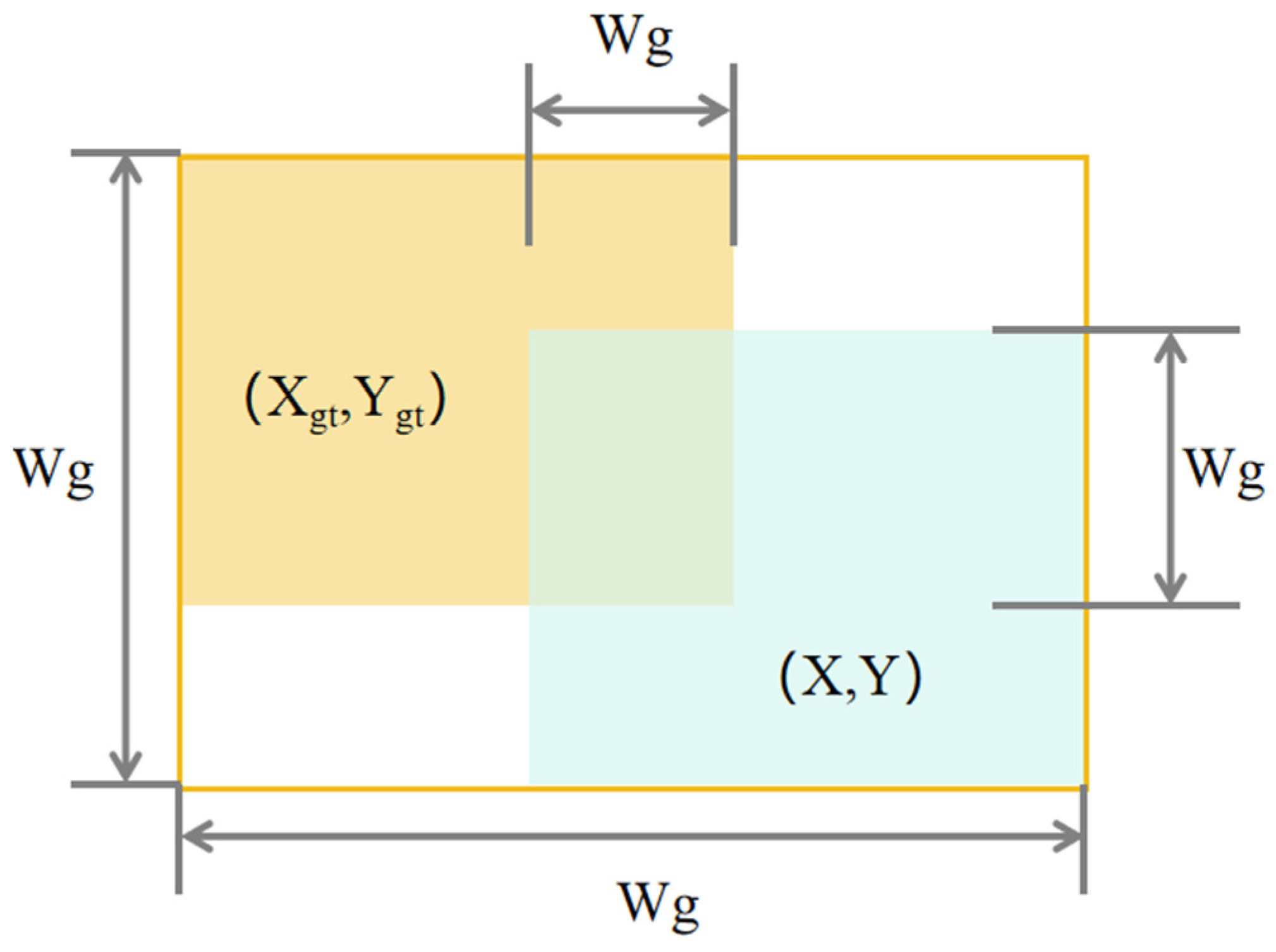
In Equation (10), the weighting factor is indicated by $\alpha$. In Equation (11), the similarity of the aspect ratios is characterized by $v$. The width and height of the real box are, respectively, represented by $w^{gt}$ and $h^{gt}$; the width, and height of the prediction box are, respectively, indicated by $w$ and $h$. The bounding box regression problem in object detection is represented in Figure 13. The orange section is the true box, and the light blue section is the predicted box. The overlap of the yellow and blue boxes is used to assess how well the predicted and true boxes match.

Although CIOU effectively solves the problem that IOU cannot handle non-overlapping bounding boxes, there are inevitably low-quality samples in the training set. Additionally, there exists some ambiguity in the aspect ratio in CIOU, and $v$ has a flaw that ignores the true relationship between width and height, affecting the speed of model convergence. The EIOU loss function is proposed to solve this problem effectively. Therefore, the EIOU loss function is adopted in our study. The EIOU is presented in Equation (12).

$$\begin{array}{c}{L}_{EIOU}=L_{IOU}+L_{dis}+L_{asp}\\ =1-IOU+{\displaystyle \frac{{\rho }^2\left(b,b^{gt}\right)}{{\left(w^c\right)}^2+{\left(h^c\right)}^2}}+{\displaystyle \frac{{\rho }^2\left(w,w^{gt}\right)}{{\left(w^c\right)}^2}}+{\displaystyle \frac{{\rho }^2\left(h,h^{gt}\right)}{{\left(h^c\right)}^2}}\end{array}$$

(12)

$L_{IOU}$ is the overlap loss, $L_{dis}$ is the center distance loss, $L_{asp}$ is the loss of width and height, $w^c$ is the minimum rectangle width that can surround the two bounding boxes, $h^c$ is the minimum rectangle height that can surround two bounding boxes.

The EIOU loss function carries over the advantages of CIOU, such as distance loss. Additionally, EIOU minimizes the gap between the width and height of the predicted and real boxes, which accelerates model convergence, making it better overall. EIOU introduces more geometric information, effectively reducing the accumulation of errors in multiple dimensions of the prediction frame. This helps the model adjust the size and position of the prediction box more accurately during training. EIOU can be adapted to multi-scale objects, making it suitable for the helmet detection scenario. Introducing GhostModule enhances the efficiency of the network structure but adversely affects its convergence speed, leading to a loss of accuracy. Therefore, we opt for the EIOU loss function to address this issue.

4. Experiment

4.1. Dataset

The EGS-YOLO proposed in this paper was tested on the SHEL5K dataset. SHEL5K is an open-source dataset consisting of 5000 images, containing images of construction workers wearing and not wearing safety helmets in various complex scenes. The dataset is divided into six classes: head, helmet, person with helmet, head with helmet, person without helmet, and face. It is a refinement of the SHD dataset, with mislabeled images corrected. Unlike other datasets, this dataset includes the additional category of face. The dataset contains 75,570 labels, with helmet having 19,252 labels, head having 6120 labels, head with helmet having 16,048 labels, person without helmet having 5248 labels, person with helmet having 14,767 labels, and face having 14,135 labels. In our experiments, we divided the dataset into training, validation, and test sets in a ratio of 8:1:1. Partial images of SHEL5K are displayed in Figure 14.

4.2. Experimental Setup

In this study, we use the development environment of Python 3.8, PyTorch 1.11.0, and CUDA 11.3. The operating system is based on Ubuntu 20.04, and the GPU is an NVIDIA RTX 3090 (24G). The input image size is 640 × 640, the initial learning rate is set to 0.01, and the optimizer is Stochastic Gradient Descent (SGD), with the SGD momentum parameter set to 0.937. The training epoch is 200, and the batch size is 16. All experiments in this paper were run on the same device. The experimental equipment is listed in

Table 1. Experimental Equipment.

Parameter	Configuration
CPU	Xeon (R) Platinum 8255C
GPU	RTX 3090 (24 G)
System environment	ubuntu20.04
Acceleration environment	CUDA11.3
Language	Python3.8

.

4.3. Evaluation Index

To comprehensively evaluate the effectiveness of the method proposed in this paper, we used multiple evaluation metrics, including widely used metrics such as Recall (R), Precision (P), parameters (params), computational complexity (FLOPs), average precision, mean average precision (mAP), and inference time (inference). The calculation formulas for Precision (P), Recall (R), average precision (AP), mean average precision (mAP), params, and FLOPs are shown below in Equations (13)–(18).

$$Precision={\displaystyle \frac{TP}{TP+FP}}$$

(13)

$$Recall={\displaystyle \frac{TP}{TP+FN}}$$

(14)

AP is the average precision and is the area below the PR curve. The higher the AP value, the more accurate the model is, as shown in Equation (15).

$$AP={\int }_0^{1}p\left(r\right)dr$$

(15)

$$mAP={\displaystyle \frac{1}{m}}\sum _n^{m}A{P}_n$$

(16)

$TP$ means that the prediction is a positive sample, and the reality is also a positive sample, called a true positive. $FP$ signifies that the predicted sample is positive, and the actual sample is negative, called a false positive. $FN$ is the sample that is predicted to be false but is actually true, known as a false negative.

$$params=C_{out}\left(H\times W\times C_{in}+1\right)$$

(17)

$$FLOPs=2C_{out}(C_{in}{K}^2+1)\times H\times W$$

(18)

$H\times W$ is the size of the input feature map, $C_{in}$ and $C_{out}$ represent the channels of the input and output feature maps respectively, and $K$ denotes the convolution kernel.

4.4. Experiment Results

The EGS-YOLO was tested on the SHEL5K dataset, and the results are presented in

Table 2. The results of EGS-YOLO on SHEL5K for each category.

Name	Precision (%)	Recall (%)	[email protected] (%)
Helmet	93.3	87.5	92.9
Head	90.4	86.8	92.1
Head with helmet	89.8	88.8	93.2
Person with helmet	90.6	85.6	92.7
Person no helmet	86.1	79	86.9
Face	89.3	80.4	88.8
All	89.9	84.7	91.1

. Among the six categories tested, the Precision (P), Recall (R), and mean average precision (mAP) ranged from 86.1% to 93.3%, 79% to 88.8%, and 86.9% to 93.2%, respectively. The overall [email protected] reached 91.1%, meeting the precision requirements for practical detection. The [email protected] for helmet, head, head with helmet, and person with helmet all exceeded 92%, demonstrating excellent accuracy. EGS-YOLO achieves high detection accuracy across all categories, making it suitable for practical use on construction sites. Additionally, the inference time, number of parameters, and computational complexity of EGS-YOLO are effectively optimized. The method exhibits outstanding performance in terms of both accuracy and inference time. The Precision and Recall plots are displayed in Figure 15, parts (a) and (b), respectively, and indicate that both metrics have reached high levels.

4.4.1. Experimentation and Selection of Attention Mechanism

To select the attention mechanism, we experimented with several popular options: SE (Squeeze-and-Excitation), SimAM (Simple Attention Mechanism), CBAM (Convolutional Block Attention Module), SHUFFLE (Shuffle Attention), and CA (Coordinate Attention). The embedding location for each attention mechanism was kept consistent, and the specific performance results are presented in

Table 3. Comparison of Experimental Results for Various Attention Mechanisms.

Method	[email protected] (%)	Params (M)	FLOPs (G)	Inference (ms)	Size (MB)
Baseline	90.9	36.5	103.2	4.5	74.9
+SE	91.6	36.8	103.6	4.5	75.5
+CBAM	91.1	36.8	103.8	14.9	75.5
+SimAM	91.4	36.5	103.3	15.1	74.9
+SHUFFLE	91.1	36.5	103.3	10.1	74.9
+CA	91.2	36.8	103.8	19.5	75.4

.

The SE attention mechanism improved the [email protected] by 0.7%, outperforming the other attention mechanisms. Importantly, the introduction of SE did not affect the model’s inference time, whereas other mechanisms had a significant negative impact on inference speed. Additionally, the increase in parameters due to the SE block was within an acceptable range. Considering all factors, we selected the SE block. The inference time reported in this paper was obtained with a batch size of 16.

4.4.2. Experimentation and Selection of Lightweight Modules

The purpose of making the model lightweight is to improve its real-time performance. When designing the lightweight model, we considered four methods: GhostModule, PConv, DSConv, and MBConv, and conducted experiments to select the best method. The positions and quantities of all added modules were kept consistent. The experimental results are shown in

Table 4. Comparison of Experimental Results for Various Lightweight Modules.

Method	[email protected] (%)	Params (M)	FLOPs (G)	Inference (ms)	Size (MB)
Baseline	90.9	36.5	103.2	4.5	74.9
+GhostModule	90.1	22.6	68.0	3.9	47.2
+PConv	90.4	24.4	72.3	4.3	50.7
+DSConv	87.7	23.4	65.6	3.8	55.4
+MBConv	90.5	25.3	75.0	4.9	52.7

.

From the experimental results in Table 4, after adopting MBConv, the [email protected] is the highest at 90.5%, but its parameters and computational complexity are also the highest compared with other modules, and the inference time is increased by 8.9%. After adopting the DSConv, although the inference time decreased the most by 15.6%, the accuracy dropped considerably, with the [email protected] at 87.7%, which is not considered acceptable. Although the [email protected] of the model is 90.1% after adopting GhostModule, which is slightly lower than MBConv and PConv, the parameters are reduced by 38.1%, the computational complexity is reduced by 34.1%, and the inference time is decreased by 13.3%. Considering all factors, GhostModule was selected. The introduction of GhostModule effectively accelerates inference, reduces the number of model parameters, and decreases computational complexity. The inference time reported in this paper was obtained with a batch size of 16.

4.4.3. Ablation Experiment

To evaluate the feasibility of our proposed method, EGS-YOLO, for helmet wear detection, we performed ablation experiments. In these experiments, the device and parameter settings were kept the same. The experimental results are presented in

Table 5. The Result of Ablation Experiment (Baseline is YOLOv7).

Method	[email protected] (%)	Params (M)	FLOPs (G)	Inference (ms)	Size (MB)
Baseline	90.9	36.5	103.2	4.5	74.9
+GhostModule	90.1	22.6	68.0	3.9	47.2
+GhostModule + SE	90.6	22.9	68.3	3.9	47.8
+GhostModule + EIOU	90.7	22.6	68.0	3.9	47.2
+GhostModule + EIOU + SE	91.1	22.9	68.3	3.9	47.8

.

After introducing GhostModule, the [email protected] of the model is 90.1%, a decrease of 0.8% compared with the baseline. The parameters are 22.6 M, a reduction of 38.1%, the computational complexity is 68.0 GFLOPs, a reduction of 34.1%, and the inference time is 3.9 ms, a reduction of 13.3%. This demonstrates that adopting GhostModule enhances real-time performance and lightens the model to some extent.

Following the integration of GhostModule, the adoption of EIOU as a loss function was evaluated. Compared with the model only introducing GhostModule, [email protected] increased by 0.6% to 90.7%, while the parameters, computational complexity, and inference time remained unchanged. EIOU loss accelerates network convergence, aiding accurate target localization and improving detection accuracy.

After replacing GhostModule and embedding the SE attention mechanism, compared with the model that only introduced GhostModule, the [email protected] increased by 0.5% to 90.6%, while the parameters and computational complexity slightly increased, and the inference time remained unchanged. The SE block makes the model more attentive to features of different scales, reducing the impact of cluttered information and enhancing feature extraction without losing detection speed.

After introducing GhostModule, SE, and EIOU into the model simultaneously, [email protected] is 91.1%, the parameters are 22.9 M, the computational complexity is 68.3 GFLOPs, and the inference time is 3.9 ms. Compared to the model only introducing GhostModule, [email protected] is 1% higher, with the parameters and computational complexity slightly increased, and the inference time unchanged. Compared with YOLOv7, [email protected] increased by 0.2%, the parameters were reduced by 37.3%, the computational complexity decreased by 33.8%, the inference time decreased by 13.3%, and the model weight was reduced by 36.2%. This indicates a slight improvement in accuracy, enhanced real-time performance, and a lighter model.

4.4.4. Comparative Experiment

To validate the advancement of EGS-YOLO, we compare it with other advanced models, including YOLOv8m, YOLOv7, YOLOv5x, YOLOv5l, YOLOv5m, and YOLOv3, as well as existing studies in terms of accuracy. The experimental results are presented in

Table 6. Comparison of EGS-YOLO with other state-of-the-art algorithms.

Method	[email protected] (%)	Params (M)	FLOPs (G)	Inference (ms)	Size (MB)
YOLOv3	87.1	61.5	154.6	10.2	123.6
Faster R-CNN	41.3	108	137	30	108.9
YOLOv5m	86.6	20.9	47.9	7.0	42.3
YOLOv5l	87	46.1	107.7	9.5	92.9
YOLOv5x	87.3	86.2	203.9	13.9	173.2
YOLOv7	90.9	36.5	103.2	4.5	74.9
YOLOv8m	89.4	25.8	78.7	7.2	52.1
Barlybayev et al. [12]	89.6	×	×	×	×
Otgonbold et al. [15]	88.28	36.9	×	×	×
EGS-YOLO	91.1	22.9	68.3	3.9	47.8

.

From Table 6, it is evident that EGS-YOLO achieves the highest [email protected], reaching 91.1%, which is 4%, 4.5%, 4.1%, 3.8%, 0.2%, and 1.7% higher than YOLOv3, YOLOv5m, YOLOv5l, YOLOv5x, YOLOv7, and YOLOv8m, respectively. EGS-YOLO is also more accurate than the models by Barlybayev and Otgonbold by 1.5% and 2.82%, respectively. EGS-YOLO has the fastest inference speed (RTX3090) at 3.9 ms, which is 6.3 ms, 3.1 ms, 5.6 ms, 10 ms, 0.6 ms, and 3.3 ms faster than YOLOv3, YOLOv5m, YOLOv5l, YOLOv5x, YOLOv7, and YOLOv8m, respectively. In terms of parameters and computational complexity, EGS-YOLO has 37.3% fewer parameters and 33.8% lower computational complexity than the baseline model YOLOv7. Compared to YOLOv8 of the same scale, EGS-YOLO is superior.

The comparison of [email protected] between YOLOv7 and EGS-YOLO is shown in Figure 16, with the horizontal axis representing the number of iterations. As shown in Figure 16, after 125 iterations, the [email protected] of EGS-YOLO gradually approaches and slightly surpasses that of YOLOv7. This indicates that EGS-YOLO maintains high accuracy while effectively improving inference time, the number of parameters, and computational complexity. EGS-YOLO has excellent performance high accuracy and high real-time performance. The test of EGS-YOLO on individual images is shown in Figure 17. From Figure 17, it can be seen that the detection accuracy basically reaches more than 90%, and some objects even reach a high accuracy of 96%, which proves the reliability of the method.

5. Conclusions

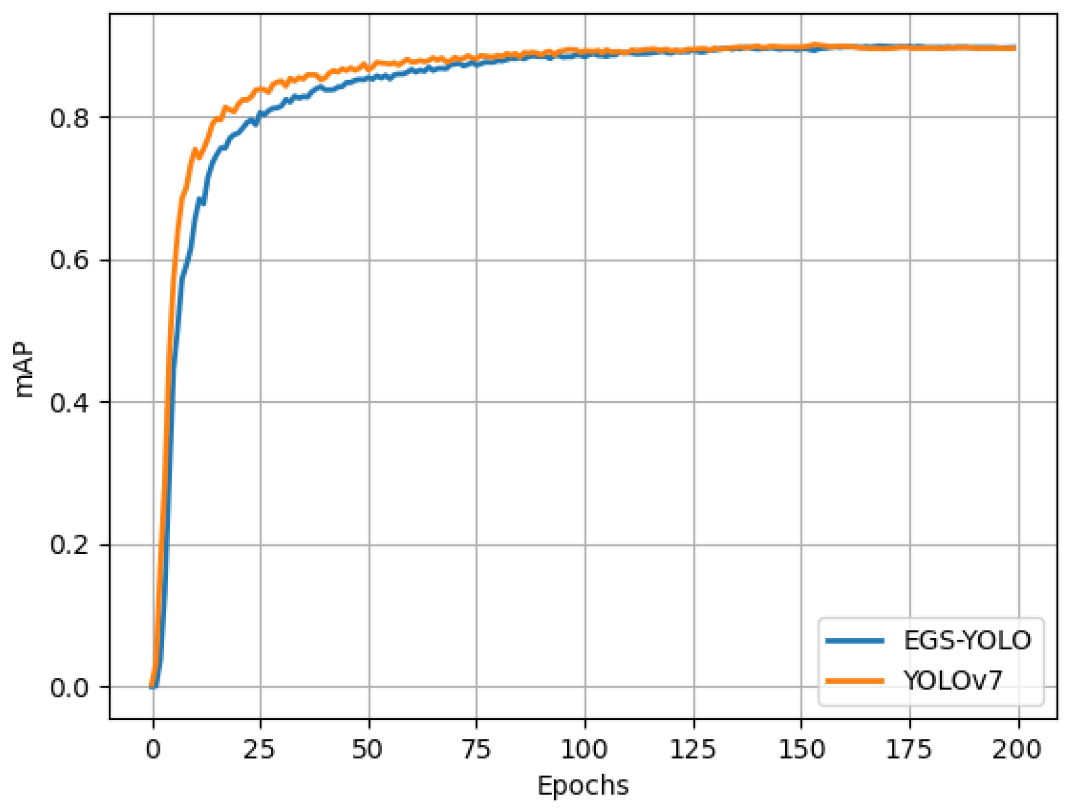
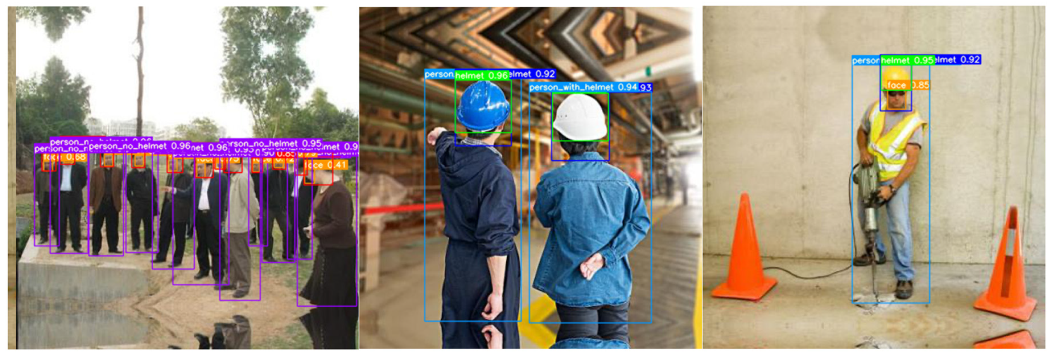
In this study, we improved YOLOv7 and successfully constructed EGS-YOLO. Compared to YOLOv7, the model boasts improved real-time performance while maintaining high precision, and it also has reduced parameters and computational complexity. Compared with the existing research, it has taken into account a variety of metrics and has excellent performance with high accuracy and high real-time performance. The GhostModule is adopted to enhance real-time performance and to lighten the model to some extent. The SE block is introduced to strengthen the model’s ability to extract valuable features and mitigate the impact of complex factors. The EIOU loss function is utilized to achieve faster convergence and more accurate localization. We successfully constructed new efficient structures such as ELAN-G, ELAN-HG, ELAN-GS, and SPPCSPC-GS. EGS-YOLO is capable of adapting to diverse and complex scenarios in helmet wear detection, achieving both high real-time and high-accuracy performance. The detection [email protected] of EGS-YOLO is 91.1%, with Precision and Recall rates of 89.9% and 84.7%, respectively. Notably, compared to YOLOv7, EGS-YOLO has a 0.2% higher [email protected], a 37.3% reduction in parameters, a 33.8% decrease in computational complexity, and an inference time of 3.9 ms, a 13.3% reduction. The EGS-YOLO proposed in this study meets the requirements for high-accuracy and high real-time detection of safety helmets on construction sites.

In future research, we will focus on optimizing the model to investigate ways to further enhance accuracy. This will be achieved by incorporating dynamic convolution, deformable convolution, and feature fusion. Additionally, we will research further lightweight models, making them lighter through model pruning and other techniques.

References

1. Park, M.-W.; Elsaft, N.; Zhu, Z. Hardhat-wearing detection for enhancing on-site safety of construction workers. J. Constr. Eng. Manag. 2015, 141, 04015024. [Google Scholar] [CrossRef]
2. Kelm, A.; Laußat, L.; Meins-Becker, A.; Platz, D.; Khazaee, M.J.; Costin, A.M. Mobile passive radio frequency identification (RFID) portal for automated and rapid control of personal protective equipment (PPE) on con-struction sites. Autom. Constr. 2013, 36, 38–52. [Google Scholar] [CrossRef]
3. Barro-Torres, S.; Fernández-Caramés, T.M.; Pérez-Iglesias, H.J.; Escudero, C.J. Real-time personal protective equipment monitoring system. Comput. Commun. 2012, 36, 42–50. [Google Scholar] [CrossRef]
4. Dong, S.; He, Q.; Li, H.; Yin, Q. Automated PPE Misuse Identification and Assessment for Safety Performance Enhancement. In Proceedings of the ICCREM, Lulea, Sweden, 11–12 August 2015; Volume 2015, pp. 204–214. [Google Scholar] [CrossRef]
5. Sun, X.; Xu, K.; Wang, S. Detection and tracking of safety helmet in factory environment. Meas. Sci. Technol. 2021, 32, 105406. [Google Scholar] [CrossRef]
6. Fang, Q.; Li, H.; Luo, X.; Ding, L.; Luo, H.; Rose, T.M.; An, W. Detecting non-hardhatuse by a deep learning method from far-field surveillance videos. Autom. Constr. 2018, 85, 1–9. [Google Scholar] [CrossRef]
7. Zhao, L.; Tohti, T.; Hamdulla, A. BDC-YOLOv5: A helmet detection model employs improved YOLOv5. Signal Image Video Process. 2023, 17, 4435–4445. [Google Scholar] [CrossRef]
8. Hayat, A.; Morgado-Dias, F. Deep Learning-Based Automatic Safety Helmet Detection System for Construction Safety. Appl. Sci. 2022, 12, 8268. [Google Scholar] [CrossRef]
9. Li, Z.; Xie, W.; Zhang, L.; Lu, S.; Xie, L. Toward Efficient Safety Helmet Detection Based on YoloV5 with Hierarchical Positive Sample Selection and Box Density Filtering. IEEE Trans. Instrum. Meas. 2022, 71, 2508314. [Google Scholar] [CrossRef]
10. Li, X.; Hao, T.; Li, F.; Zhao, L.; Wang, Z. Faster R-CNN-LSTM Construction Site Unsafe Behavior Recognition Model. Appl. Sci. 2023, 13, 10700. [Google Scholar] [CrossRef]
11. Fu, Z.; Ling, J.; Yuan, X.; Li, H.; Li, H.; Li, Y. Yolov8n-FADS: A Study for Enhancing Miners’ Helmet Detection Accuracy in Complex Underground Environments. Sensors 2024, 24, 3767. [Google Scholar] [CrossRef] [PubMed]
12. Barlybayev, A.; Amangeldy, N.; Kurmetbek, B.; Krak, I.; Razakhova, B.; Tursynova, N. Personal protective equipment detection using YOLOv8 architecture on object detection benchmark datasets: A comparative study. Cogent Eng. 2024, 11, 2333209. [Google Scholar] [CrossRef]
13. He, C.; Tan, S.; Zhao, J.; Ergu, D.; Liu, F.; Ma, B.; Li, J. Efficient and Lightweight Neural Network for Hard Hat Detection. Electronics 2024, 13, 2507. [Google Scholar] [CrossRef]
14. Xu, H.; Wu, Z. MCX-YOLOv5: Efficient helmet detection in complex power warehouse scenarios. J. Real-Time Image Proc. 2024, 21, 27. [Google Scholar] [CrossRef]
15. Otgonbold, M.-E.; Gochoo, M.; Alnajjar, F.; Ali, L.; Tan, T.-H.; Hsieh, J.-W.; Chen, P.-Y. SHEL5K: An Extended Dataset and Benchmarking for Safety Helmet Detection. Sensors 2022, 22, 2315. [Google Scholar] [CrossRef] [PubMed]
16. Wang, C.; Bochkovskiy, A.; Liao, H.M. YOLOv7: Trainable bag-of-freebies sets new state-of-the-art for real-time object detectors. In Proceedings of the 2023 IEEE/CVF Conference on Computer Vision and Pattern Recognition (CVPR), Vancouver, BC, Canada, 18–22 June 2023; pp. 7464–7475. [Google Scholar]
17. Girshick, R.; Donahue, J.; Darrell, T. Rich feature hierarchies for accurate object detection and semantic segmentation. In Proceedings of the IEEE Conference on Computer Vision and Pattern Recognition, 23–28 June 2014; pp. 580–587. [Google Scholar] [CrossRef]
18. Girshick, R. Fast R-CNN. In Proceedings of the IEEE International Conference on Computer Vision, Santiago, Chile, 7–13 December 2015; pp. 1440–1448. [Google Scholar] [CrossRef]
19. Ren, S.; He, K.; Girshick, R.; Sun, J. Faster R-CNN: Towards Real-Time Object Detection with Region Proposal Networks. In Proceedings of the IEEE Transactions on Pattern Analysis and Machine Intelligence, Montreal, QC, Canada, 7–12 December 2015. [Google Scholar] [CrossRef]
20. Liu, W.; Anguelov, D.; Erhan, D.; Szegedy, C. SSD: Single Shot MultiBox Detector. In Computer Vision—ECCV 2016; Springer: Cham, Switzerland, 2016. [Google Scholar]
21. Redmon, J.; Divvala, S.; Girshick, R. You only look once: Unified, real-time object detection. In Proceedings of the IEEE Conference on Computer Vision and Pattern Recognition, Las Vegas, NV, USA, 27–30 June 2016; pp. 779–788. [Google Scholar]
22. Howard, A.G.; Zhu, M.; Chen, B.; Kalenichenko, D.; Wang, W.; Weyand, T. Mobilenets: Efficient convolutional neural networks for mobile vision applications. arXiv 2017, arXiv:1704.04861. [Google Scholar]
23. Sandler, M.; Howard, A.; Zhu, M.; Zhmoginov, A.; Chen, L.C. Mobilenetv2: Inverted residuals and linear bottlenecks. In Proceedings of the IEEE Conference on Computer Vision and Pattern Recognition, Salt Lake City, UT, USA, 18–23 June 2018; pp. 4510–4520. [Google Scholar]
24. Howard, A.; Sandler, M.; Chu, G.; Chen, L.-C.; Chen, B.; Tan, M. Searching for mobilenetv3. In Proceedings of the 2019 IEEE/CVF International Conference on Computer Vision (ICCV 2019), Seoul, Republic of Korea, 27 October–2 November 2019. [Google Scholar]
25. Tan, M.; Le, Q. Efficientnetv2: Smaller models and faster training. In Proceedings of the International Conference on Machine Learning (ICML), Virtual Event, 18–24 July 2021; pp. 10096–10106. [Google Scholar]
26. Nascimento, M.G.D.; Prisacariu, V.; Fawcett, R. DSConv: Efficient Convolution Operator. In Proceedings of the 2019 IEEE/CVF International Conference on Computer Vision (ICCV), Seoul, Republic of Korea, 27 October–2 November 2019; pp. 5147–5156. [Google Scholar] [CrossRef]
27. Chen, J.; Kao, S.-H.; He, H.; Zhuo, W.; Wen, S.; Lee, C.H. Run, Don’t Walk: Chasing Higher FLOPS for Faster Neural Networks. arXiv 2023, arXiv:2303.03667. [Google Scholar]
28. Han, K.; Wang, Y.; Tian, Q. Ghostnet: More features from cheap operations. In Proceedings of the IEEE/CVF Conference on Computer Vision and Pattern Recognition (CVPR), Seattle, WA, USA, 13–19 June 2020; pp. 1580–1589. [Google Scholar]
29. Hassanin, M.; Anwar, S.; Radwan, I.; Khan, F.; Mian, A. Visual attention methods in deep learning: An in-depth survey. Inf. Fusion 2024, 108, 102417. [Google Scholar] [CrossRef]
30. Hu, J.; Shen, L.; Sun, G. Squeeze-and-excitation networks. In Proceedings of the IEEE Conference on Computer Vision and Pattern Recognition, Salt Lake City, UT, USA, 18–23 June 2018; pp. 7132–7141. [Google Scholar]
31. Zhu, X.; Cheng, D.; Zhang, Z.; Lin, S.; Dai, J. An Empirical Study of Spatial Attention Mechanisms in Deep Networks. In Proceedings of the 2019 IEEE/CVF International Conference on Computer Vision (ICCV), Seoul, Republic of Korea, 27 October–2 November 2019; pp. 6687–6696. [Google Scholar]
32. Woo, S.; Park, J.; Lee, J.Y. CBAM: Convolutional block attention module. In Proceedings of the European Conference on Computer Vision (ECCV), Munich, Germany, 8–14 September 2018; Lecture Notes in Computer Science. IEEE: Piscataway, NJ, USA, 2018; pp. 3–19. [Google Scholar]
33. Zheng, Z.; Wang, P.; Liu, W.; Li, J.; Ye, R.; Ren, D. Distance-iou loss: Faster and better learning for bounding box regression. In Proceedings of the AAAI Conference on Artificial Intelligence, New York, NY, USA, 7–12 February 2020; Volume 34, pp. 12993–13000. [Google Scholar] [CrossRef]
34. Zhang, Y.F.; Ren, W.; Zhang, Z. Focal and efficient iou loss for accurate bounding box regression. Neurocomputing 2022, 506, 146–157. [Google Scholar] [CrossRef]
Figure 1. The whole structure of YOLOv7.
Applsci 14 07923 g001
Figure 2. The structure of CBS.
Applsci 14 07923 g002
Figure 3. The structure of ELAN.
Applsci 14 07923 g003
Figure 4. The structure of ELAN-H.
Applsci 14 07923 g004
Figure 5. The structure of MP.
Applsci 14 07923 g005
Figure 6. The structure of SPPCSPC.
Applsci 14 07923 g006
Figure 7. The process of ordinary convolution.
Applsci 14 07923 g007
Figure 8. The process of GhostModule.
Applsci 14 07923 g008
Figure 9. The structure of ELAN-G, ELAN-HG, and SPPCSPC-G (G is the GhostModule).
Applsci 14 07923 g009
Figure 10. The structure of SE (Squeeze-and-Excitation).
Applsci 14 07923 g010
Figure 11. The structure of ELAN-GS and SPPCSPC-GS (G is the GhostModule and S is the SE).
Applsci 14 07923 g011
Figure 12. The structure of the improved model EGS-YOLO (E is EIOU loss function, G is GhostModule, S is SE block).
Applsci 14 07923 g012
Figure 13. Predict box and true box (the yellow part is the true box, and the light blue part is the predict box).
Applsci 14 07923 g013
Figure 14. A section of images from SHEL5K.
Applsci 14 07923 g014
Figure 15. Precision and Recall plots of EGS-YOLO on SHEL5K dataset. (a) is the Precision curve. (b) is the Recall cure.
Applsci 14 07923 g015
Figure 16. Curves comparison of the [email protected] of EGS-YOLO and YOLOv7.
Applsci 14 07923 g016
Figure 17. The detection results of EGS-YOLO to some images from SHEL5K.
Applsci 14 07923 g017