
Active Learning for Biomedical Article Classification with Bag of Words and FastText Embeddings


Institute of Computer Science, Warsaw University of Technology, 00-665 Warsaw, Poland
Appl. Sci. 2024, 14(17), 7945; https://doi.org/10.3390/app14177945
Submission received: 24 July 2024
/
Revised: 27 August 2024
/
Accepted: 2 September 2024
/
Published: 6 September 2024
(This article belongs to the Special Issue Data and Text Mining: New Approaches, Achievements and Applications)
Abstract
:In several applications of text classification, training document labels are provided by human evaluators, and therefore, gathering sufficient data for model creation is time consuming and costly. The labeling time and effort may be reduced by active learning, in which classification models are created based on relatively small training sets, which are obtained by collecting class labels provided in response to labeling requests or queries. This is an iterative process with a sequence of models being fitted, and each of them is used to select query articles to be added to the training set for the next one. Such a learning scenario may pose different challenges for machine learning algorithms and text representation methods used for text classification than ordinary passive learning, since they have to deal with very small, often imbalanced data, and the computational expense of both model creation and prediction has to remain low. This work examines how classification algorithms and text representation methods that have been found particularly useful by prior work handle these challenges. The random forest and support vector machines algorithms are coupled with the bag of words and FastText word embedding representations and applied to datasets consisting of scientific article abstracts from systematic literature review studies in the biomedical domain. Several strategies are used to select articles for active learning queries, including uncertainty sampling, diversity sampling, and strategies favoring the minority class. Confidence-based and stability-based early stopping criteria are used to generate active learning termination signals. The results confirm that active learning is a useful approach to creating text classification models with limited access to labeled data, making it possible to save at least half of the human effort needed to assign relevant or irrelevant class labels to training articles. Two of the four examined combinations of classification algorithms and text representation methods were the most successful: the SVM algorithm with the FastText representation and the random forest algorithm with the bag of words representation. Uncertainty sampling turned out to be the most useful query selection strategy, and confidence-based stopping was found more universal and easier to configure than stability-based stopping.
1. Introduction
Text classification has become one of the most extensively studied research areas within machine learning and natural language processing as well as one of the most pursued practical application directions [1,2,3,4,5,6]. Texts from many different sources have been classified in these research studies and applications, including email messages, online chats, website contents, blog posts, forum discussions, customer opinions, product reviews, or scientific articles.
1.1. Motivation
One noteworthy application of text classification is to the automation of the systematic literature review (SLR) process, where articles are classified as relevant or irrelevant to a particular study topic [7,8]. Training data for creating such models are obtained by assigning class labels to a set of articles by human evaluation. Classification models are then created using machine learning algorithms, which are either conventional or based on deep neural network architectures. The former require transforming text data to a vector representation, and the latter create their own internal representations.
The time and effort required to perform the human screening of training data may be reduced by active learning [9,10]. This is an iterative process in which a sequence of models is created with each of them used to select additional training instances for the next one from the available unlabeled dataset. The general principle is to select instances believed to be the most likely to permit obtaining a better model in the next iteration. The learning system issues a class query for the selected articles, i.e., requests human-assigned class labels for them. Active learning makes it possible to create classification models of satisfactory quality using considerably less training data (and therefore requiring considerably less human effort) than in standard passive learning, but it requires appropriate criteria for query selection and stopping the process.
While scientific article classification with respect to relevance may appear less demanding than for other types of text, it is associated with some inherent specific challenges, such as limited training data availability (to be labeled, an article needs to be screened by a human expert to determine its relevance to a particular topic), poor class separation (relevant and irrelevant articles are both from the same domain and discriminating between them may be sometimes difficult even for a human evaluator), class imbalance (relevant articles are often sparse), and high computational efficiency requirements (model creation may be necessary multiple times during an interactive session with the user). While active learning reduces the human screening effort, it actually increases challenges faced by the adopted text representation methods and classification algorithms, since they have to deal with very tiny and often heavily imbalanced data and create models in practically no time. This may favor conventional machine learning algorithms for tabular data rather than deep learning neural networks [11], which are harder to use successfully with small and imbalanced training sets as well as much more computationally demanding. Also, most active learning methods known from the literature have been developed and studied for conventional machine learning algorithms [12]. The quality of models that such algorithms can produce may heavily depend on the type and dimensionality of text representation, but for the most effective algorithms and the most useful representations, it may be as good as or better than that achieved by deep neural models [13].
1.2. Related Work
Active learning for text classification has been a relatively popular research topic during the last two decades, and reviewing even a fraction of the most impactful prior work would require more space than this entire article. To provide a minimal necessary research context, Table 1 lists a small number of selected particularly closely related publications, summarizing them along the following dimensions:
Representations:
text representation methods;
Algorithms:
classification algorithms;
AL Setup:
active learning setup: initialization, query selection, and early stopping criteria;
Evaluation:
predictive performance measures and evaluation procedures;
Data:
datasets.
The common features of most of this prior work are using the bag of words text representation and uncertainty sampling for query selection. The latter appeared in several different variations, depending on the adopted uncertainty measure or some specific properties of the classification algorithm used. This is the case, in particular, for [17] using the predictions of multiple models on data packets to estimate uncertainty, [18] proposing an uncertainty sampling strategy specifically designed for a regular expression-based text classification algorithm, and [21] using a Monte-Carlo dropout uncertainty estimation technique for a deep neural network model. Researchers using the SVM algorithm often adopt query selection strategies based on the classification margin (distance to the decision boundary) [14,20]. In some studies of active learning for systematic literature reviews a query strategy that selects articles with the highest probability of being relevant to the study topic was used [16,19,22,23]. This is referred to as minority sampling in Table 1 and thereafter.
It can be easily noticed that initial training set selection has not received very much attention in prior research on active learning for text classification. Out of ten publications listed in Table 1 only one uses a non-random clustering-based initialization method [15]. The same can be said about early stopping criteria: most prior work continues the learning process until a predetermined number of iterations or instances labeled, with [18] being a single exception. While some of those studies use k-fold cross-validation for predictive performance evaluation, most settle for the less reliable train–test split approach. More importantly, predictive performance indicators are usually limited to those measuring the quality of class label predictions (e.g., accuracy, precision, recall, F1) rather than class probability or decision value predictions, although the latter would clearly provide a more complete and useful assessment of the model’s predictive utility.
Prior research specifically addressing the application of active learning to creating text classification models for systematic literature reviews usually focuses on SLR-specific performance measures. This is the case for [19,22,23], which use the work saved over sampling (WSS) metric [24], as well as time to discovery (TD) and relevant records found (RRF). These studies do not use k-fold cross-validation or train–test splitting, but rather evaluate the performance on the entire dataset, combining known true class labels (for articles labeled as relevant or irrelevant by the human evaluator) and model predictions (for unlabeled articles). This scheme is referred to as train+pool evaluation in Table 1. By the way, these three studies employ the ASReview system for systematic reviews [19] and report results obtained with text representations, algorithms, and AL setups available there. The row for [19] in Table 1 only describes the scope of the demonstration experiments reported in the article, but ASReview functionality is considerably broader.
While most of the related prior research used conventional machine learning algorithms, there have been also attempts to use deep learning models to create text classification models, including the BERT language model fine-tuned for classification [21] or a convolutional neural network [23]. While the former achieved good classification quality, it exhibited only a rather limited improvement during active learning. The latter generally worked on par with conventional algorithms.
1.3. Contributions
Although related prior work has contributed several useful ideas and results, not only exploring different classification algorithms and active learning setups, but also proposing novel custom variations thereof, it has left some noticeable gaps that this article is intended to partially fulfill. It examines how classification algorithms and text representation methods that have been found particularly useful by prior work handle the challenges associated with active learning of text classification models and with what active learning setups they work best. While the scope of the presented study is limited to only two popular and highly successful algorithms and two text representation methods, this limitation is well justified by the recent evaluation [13] in which these were found to provide the best level of prediction quality. Limiting the scope of classification algorithms and text representations to the most promising ones makes it possible to experiment with several different active learning setups on multiple datasets and systematically evaluate the predictive performance.
The experiments presented in this article are supposed to verify the scale of data labeling effort savings possible by different active learning configurations without sacrificing classification quality, i.e., to determine how the predictive performance of models obtained by active learning at different stages of this process compares to that of models that could be obtained by standard passive learning if all class labels were available. They also investigate the possibility of reliably determining when to stop the active learning process and avoid further labeling queries without sacrificing the predictive performance. The distinguishing features of this work are summarized below.
- Several different active learning setups are examined, including not only different query selection strategies, but also different initialization methods and early stopping criteria.
- A collection of 15 datasets consisting of scientific article abstracts from biomedical systematic literature review studies, of varying size and class imbalance ratio, is used for the experiments.
- The prediction quality is rigorously evaluated using -fold cross-validation with the area under the precision-recall curve adopted as the quality measure. In addition, potential workload reduction in an SLR process is estimated using the WSS measure.
2. Materials and Methods
Text representation methods, classification algorithms, and active learning setups used by this work are described in the corresponding subsections below.
2.1. Text Representation Methods
Applying conventional machine learning algorithms for tabular data to text documents requires transforming them to a vector representation in which each document is assigned values of a fixed, common set of attributes [29,30]. A document is then represented by a fixed-dimensionality vector of attribute values. This work uses both the standard bag of words representation and a representation based on word embeddings, i.e., transformations that map single words or sequences of words into a multidimensional real-valued vector space.
2.1.1. Bag of Words
The simplest vector text representation that still remains a standard choice in most text classification applications is the bag of words (BOW) representation [1,2,27], with attributes directly corresponding to words, which are also referred to as terms. In the most common term frequency (TF) variant, the value of the attribute corresponding to a term is the number of its occurrences in a given document. In the TF-IDF variant, term frequencies are normalized by inverse document frequencies (IDFs) to downweight terms occurring in many documents and upweight more unique terms [31].
The bag of words representation is order- and context-insensitive—it always treats treats all occurrences of the same term in the same way. Therefore, its capability of preserving semantic information is limited, but it can be directly interpreted, is easy to use, and works well in many applications.
2.1.2. FastText
The general common idea of word embeddings is to map words to vectors in such a way that similarity in the vector space corresponds to the semantic similarity of the words. This originates from the word2vec algorithm [32], which trains a two-layer neural network for predicting relationships between word occurrences within a fixed-length context windows, and it provides hidden layer weights as embedding vectors.
The FastText algorithm can be considered an extension of word2vec that adopts a similar approach but takes it down to the character level [28]. It creates word embeddings by training a two-layer neural network to represent a mapping between words and subwords (character n-grams, typically for n values between 3 and 6) and their context in one of the following two possible modes:
Continuous bag of words (CBOW):
predicting a target word or subword based on words or subwords occurring in the corresponding context window;
Skip-gram (SG):
predicting a target word or subword based on another single nearby word or subword.
Of those, the latter tends to work better with subword information.
Embedding vectors are obtained from hidden layer weights by summing up weights corresponding to a given word and its subwords. For sentences, paragraphs, or other word sequences, embedding vectors are obtained by averaging L2-normalized vectors for individual words in the sequence. Since words that are morphologically similar have some shared character n-grams, their resulting FastText representations are partially shared. This is how the algorithm more effectively uses training data—it can obtain useful word embeddings even from relatively small datasets and even from rarely occurring or previously unseen words. This makes it well suited to creating custom domain-specific text representations and applying a classification model using text representation derived from available data to a new dataset.
2.2. Classification Algorithms
This work uses selected classification algorithms for tabular data that have proved useful for text classification. Their advantages include good overfitting resistance and limited sensitivity to hyperparameter settings, which makes them well suited to classification tasks with high input dimensionality and relatively small training data.
2.2.1. Support Vector Machines
The support vector machine (SVM) algorithm identifies a linear decision boundary between classes that maximizes the classification margin subject to class separation constraints [26,33,34]. The constraints are usually relaxed to permit some incorrectly classified instances. Implicit input space transformation by kernel functions makes it possible to represent nonlinear decision boundaries. Signed distances of classified instances to the decision boundary serve as numeric decision function values. They can be also transformed to class probability predictions by Platt’s scaling, i.e., applying a logistic transformation with parameters adjusted for maximum likelihood [35].
2.2.2. Random Forest
The random forest (RF) algorithm creates an ensemble of decision trees, grown based on multiple bootstrap samples drawn with replacement from the training set, with randomized split selection [25]. It is an extension of bagging [37], in which the diversity of individual models in the ensemble is additionally stimulated by randomization. Prediction is performed by voting with vote distribution used to obtain class probability predictions.
Combining multiple diverse trees often provides a very good level of predictive quality and high overfitting resistance. Low sensitivity to hyperparameter settings, such as the number of trees or the number of attributes randomly drawn for split selection, makes the algorithm easy to use. It has been successfully applied to text classification with both bag of words and word embeddings representations [36,38,39,40].
2.3. Active Learning
Active learning is a form of supervised learning in which training information is provided by answers to labeling queries issued by the learning system [9,10]. A sequence of models is created iteratively with each model used to select query instances to be added to the training set for the next model. With an appropriate selection method, model quality would tend to improve in subsequent iterations to a greater extent than by adding randomly selected instances, and a satisfactory model may be reached after labeling a fraction of the available data. This is an attractive approach to classification tasks in which providing class labels requires considerable human effort, including in particular text classification [14].
2.3.1. Scenario
The active learning scenario adopted by this work is presented in Algorithm 1. It assumes there is a pool of unlabeled instances, designated by U, from which the learner selects initial training instances and requests class labels for them from the external evaluator. Then, in each iteration, the current training set T is used to create a classification model h. The learner then selects a subset of query instances Q from the pool and requests class labels for them. They are then added to the training set for the next iteration. The process is terminated when a specified maximum number of iterations has been reached, there are no more instances left in the pool, or some other stopping criteria are satisfied.
| Algorithm 1 Active learning scenario |
|
2.3.2. Initial Training Set Selection
In the course of active learning, instances for class label queries are usually selected based on the current model, choosing those that are believed to permit the greatest improvement of the next model. This is not possible when the initial training set has to be selected to create the first model. In this work, two initialization methods are used for this purpose:
Random:
random selection;
Cluster:
selection based on data clustering.
The random initialization method is simple, easy to use, and may work quite well. The cluster method additionally used by this study to verify whether it pays off to invest more effort in initial training set selection is adopted from [41]. It applies the fuzzy c-means clustering algorithm [42] to cluster pool instances and then selects a specified number of instances with the highest level of cluster membership (cluster-center selection) as well as a specified number of instances with the least difference of membership values for two different clusters (cluster-border selection). To mitigate the problem of vanishing dissimilarity differences in high-dimensional spaces, the dimensionality is reduced using PCA [43]. This was not needed in the original method of [41], which was applied to tabular data with low dimensionality.
2.3.3. Query Selection
Ideally, at each active learning iteration, class labels should be requested for those instances which would contribute the most to model quality improvement. Several query selection heuristics are known in the literature that attempt to approximate this ideal criterion [44]. Some of them are only applicable to particular classification algorithms or model representations. For this work, using two substantially different classification algorithms, algorithm-independent strategies are of greater interest. These include the following:
Uncertainty sampling:
selecting instances about which the current model is the most uncertain;
Diversity sampling:
selecting instances that differ from those already in the training set the most;
Minority sampling:
selecting instances with the highest minority class probability;
Threshold sampling:
selecting instances with the minority class probability closest to a specified threshold;
Random:
uniform random sampling used as a comparison baseline.
Uncertainty sampling assumes that the training instances that are the hardest to classify by the current model are also the most likely to improve model quality. Class probability predictions are used to identify instances in the pool with the highest prediction uncertainty. Several uncertainty measures can be applied for this purpose [45], but for binary classification with models providing class probability predictions, as assumed by this work, uncertainty sampling reduces to selecting instances for which the predicted probability of the more probable class is the closest to , i.e.,
where is the predicted probability of the more probable class for instance x.
Diversity sampling is motivated by the expectation that the most useful new training instances would be maximally different from those previously added to the training set. This strategy selects instances from the pool with the highest minimum dissimilarity to instances in the training set:
where denotes the dissimilarity between instances x and .
Minority sampling is applicable when classes are expected to be heavily imbalanced and attempts to compensate for the imbalance by selecting instances that are likely to represent the minority class. These are identified as instances from the pool with maximum predicted minority class probabilities:
where is the predicted probability of the minority class for instance x. This strategy is sometimes referred to as certainty-based sampling [16,19,23].
Threshold sampling is another approach to compensating for class imbalance during query selection. It can be considered a modified version of uncertainty sampling, which takes into account that with heavily imbalanced classes, similar class probability values close to may not actually correspond to the most uncertain predictions. A smaller probability threshold is assumed instead, and instances for which the predicted minority class probability is the closest to this threshold are selected:
2.3.4. Early Stopping Criteria
To fully achieve the benefits of active learning, consisting of reducing the amount of labeled data required to reach a satisfactory model, early stopping criteria are desirable that could be used to terminate the process before reaching the maximum number of iterations or labeled data instances. Ideally, they would detect when further model quality improvement is impossible or very unlikely. The most direct approach of evaluating model predictive performance at each active learning iteration is not necessarily reasonable and can be often hardly possible at all. This is because it requires that some labeled instances be available and hold out from model creation to be used for model evaluation only. Given the fact that it is the limited availability of training data that makes active learning useful in the first place, the abundance of labeled data permitting its use for stopping criteria cannot be assumed. Reducing the small initial training set or using some of the query instances for this purpose would probably significantly reduce the quality of the model created by active learning, therefore undermining its purpose. This is why two other types of active learning stopping criteria are considered in this work:
Confidence-based stopping:
terminating the active learning process if the observed confidence of model predictions is sufficiently high;
Stability-based stopping:
terminating the active learning process if the observed stability of model predictions is sufficiently high.
Each of these types of early stopping criteria, which are described in more detail below, can be based on model predictions obtained either on the same pool of instances as used for query selection or on a separate stop set. The latter may yield more reliable results [46], but sparing a subset of data for stopping criteria is inconvenient and, for relatively small datasets, may negatively impact model quality. To avoid premature stopping signals, the adopted criterion may be considered satisfied only after the underlying condition was true for a specified minimum number of consecutive iterations.
2.3.5. Confidence-Based Stopping
Confidence is assessed based on class probability predictions and can be considered the opposite of uncertainty (and often measured by 1’s complement of uncertainty measures). By aggregating confidence values over all pool instances, one obtains a measure of the model’s confidence over the entire pool. The mean or the minimum are typically used for this aggregation, and the stopping criterion is considered satisfied if the mean or minimum confidence rises above a specified threshold [47]. For this work, the minimum aggregation is adopted, and prediction confidence is measured by the probability of the most probable class. For improved reliability, the criterion is considered satisfied if the underlying condition is met for a fixed number of consecutive iterations.
2.3.6. Stability-Based Stopping
Stability-based stopping criteria are based on comparing model predictions from two consecutive iterations and measuring their level of similarity. One straightforward way to do this using class label predictions would be by the share of instances for which the predicted classes differ [48]. However, with models providing class probability predictions or decision function values, it may be more appropriate to rather use those to assess stability. The approach assumed in this work is to calculate the linear correlation between predicted class probabilities from two consecutive iterations and consider the criterion satisfied if it exceeds a specified threshold and this situation persists for a fixed number of consecutive iterations.
3. Results
The experimental study applies active learning as presented Section 2.3 with text representation methods reviewed in Section 2.1 and classification algorithms briefly described in Section 2.2 to datasets from biomedical systematic literature review studies. The most important question this work attempts to answer is how the predictive performance of models obtained by several active learning configurations at different stages of this process compares to that of models that could be obtained by standard passive learning if all class labels were available. A secondary related question is whether it is possible to reliably determine when to stop the active learning process and save the effort of providing class labels without sacrificing the predictive performance. To answer these two questions, both aggregated results (averaged over multiple datasets) for all examined algorithm configurations and detailed results for selected most useful configurations are presented.
3.1. Datasets
The experiments use data from drug class review studies first introduced by [24] to evaluate the performance of text classification applied to SLR, (currently available from [49]) and then used in several other publications [50,51,52,53,54]. There are 15 study topics with the corresponding sets of article PubMed identifiers labeled as relevant or irrelevant by human evaluators based on their abstracts. Using these label assignments, datasets with article abstracts from the MEDLINE database and class labels were prepared. Combining article abstracts with relevant/irrelevant class labels for 15 topics yields therefore 15 datasets for text classification.
The size and class distribution of each of the 15 datasets is presented in Table 2. They differ slightly from those reported by [24] due to possible changes of the MEDLINE records or differences in the matching procedure. All the datasets are imbalanced, some quite heavily, which is to be expected in the case of systematic literature review studies, with relevant articles several times or even dozens of times less frequent than irrelevant articles.
3.2. Algorithm Implementations and Setup
The experimental study was performed in the Python language environment using software libraries providing implementations of text representation methods and classification algorithms. A custom implementation of the active learning process was developed to permit sufficient control of initialization, query selection, and early stopping criteria as well as adequate model evaluation.
3.2.1. Text Representation Methods
The implementation and setup details for two types of text representation described in Section 2.1 are provided below.
Bag of Words (BOW)
The CountVectorizer class from the scikit-learn Python library [55] is used to implement the bag of words representation. The minimum and maximum document frequency for a word to be included in the vocabulary were set to common-sense values and , respectively, resulting in a moderate vocabulary size (typically of several hundred words). Basic text preprocessing was performed with tokenization, non-word, and stop-word removal using the spaCy Python library [56]. Using TF-IDF instead of raw term frequencies or performing lemmatization was found not to have much effect in prior work with the same data [13], and therefore, these alternative variants of the bag of words representation are not investigated here.
FastText (FT)
Custom FastText vectors were trained using the fasttext Python library [57] with vector dimensionality set to 100, skip-gram training mode, and other parameters left at their default settings. Combined data from all SLR studies were used for embedding training, which had been previously found superior to both using publicly available pretrained vectors or training separate embeddings for each dataset [13].
3.2.2. Classification Algorithms
The following implementations of classification algorithms described in Section 2.2 provided by the scikit-learn Python library [55] were used:
SVM:
class SVC with radial kernel, balanced class weighting, and other hyperparameters left at default settings, with data standardization performed using the StandardScaler class;
RF:
random forest, class RandomForestClassifier with 500 trees, balanced class weighting, and other other hyperparameters left at default settings.
While some settings were manually adjusted, as specified above, no hyperparameter tuning was performed. This is motivated not only by the small size of the available datasets but also—and more importantly—by the desire to ensure the full realism of the experimental procedure, which should match the actual conditions of potential applications (in particular, to systematic literature reviews). The extremely limited availability of labeled data, which is the primary reason for using active learning learning in the first place, would make hyperparameter tuning hardly possible, and therefore, it is more useful to examine the classification quality possible to obtain with mostly default settings. It is also worthwhile to note that if hyperparameter tuning were to be performed, a separate test set or an external cross-validation loop would be needed for reliable predictive performance evaluation. Otherwise, classification quality estimates might be overoptimistic. Given the small data size, as in the presented experimental study (and as typically encountered in systematic literature review applications), saving some data for final model evaluation after hyperparameter tuning would be problematic and have potentially harmful effects on model quality and evaluation reliability, outweighing the benefits of tuning.
3.2.3. Active Learning
The implementation of active learning developed for this work follows the scenario presented in Section 2.3, and it adopts the initialization methods, the query selection strategies, and the early stopping criteria described there. The initial training size and the number of query instances per iteration are set relative to the overall data size as about 5% and 1%, respectively. For cluster initialization, the proportion of cluster border to cluster center instances is 2:1. The threshold sampling query selection method is used with a probability threshold value of .
The early stopping criteria are checked at each iteration using the remaining pool of unlabeled instances, without a separate stopping set, to avoid additionally reducing the small number of instances available for model creation and evaluation, and they are considered satisfied if the underlying confidence or stability condition is met for three consecutive iterations. Whenever it happens, the active learning process is not actually stopped, and just the corresponding iteration number is retained. This makes it possible to observe the predictive performance at iterations when different early stopping criteria were satisfied as well as at iterations corresponding to different percentages of the pool having been used. Multiple threshold values for each type of the stopping criteria are used:
confidence:
, , , , , , ,
stability:
.
Another noteworthy feature of the active learning implementation is that a test or validation set may be specified to which the current model is applied at each active learning iteration and the predictive performance is evaluated. This makes it possible to combine active learning with external cross-validation, as it will be discussed below.
3.3. Predictive Performance Evaluation
The primary focus of the experiments is on the effects of active learning in different configurations on the classification quality achieved by the resulting models. Despite using data from systematic literature reviews, this article does not present and investigate an actual SLR application. That being said, some limited evaluation of the SLR workload reduction is also included for the sake of completeness.
3.3.1. Classification Quality
This work evaluates classification quality using precision–recall (PR) analysis to measure the predictive performance over all possible operating points, corresponding to all possible tradeoffs between the precision and the recall. The overall performance can be summarized using the area under the precision–recall curve (PR AUC), which is the average precision across the whole range of recall values. It is much more sensitive to incorrect positive class predictions than the more common ROC analysis [58,59] and therefore provides more reliable classification quality evaluation and better detection of performance differences between algorithm configurations under class imbalance.
For reliable prediction quality evaluation, the -fold cross-validation (-CV) procedure is applied [60], with and . The true class labels and predictions for all iterations are then combined to determine the PR curves and the corresponding AUC values.
The active learning process uses each training subset of -CV as its pool of unlabeled instances from which the initial training set and instances for class label queries are selected. The test subsets of each -CV fold are used to evaluate the predictive performance of models from all active learning iterations. The iteration numbers at which particular stopping criteria were satisfied are averaged over all cross-validation folds.
3.3.2. SLR Workload Reduction
To evaluate the workload reduction possible to obtain in an SLR process, the work saved over sampling (WSS) metric is used, which represents the share of irrelevant articles that would not have to be manually screened (because they were correctly identified by the classification model) over a random sampling baseline. However, the original definition of WSS [24] was not intended for active learning and does only take into account the human effort of screening articles classified as relevant, ignoring the effort needed to provide training data labels. To account for the latter, the WSS is defined as
where, after [61]
Here, N is the total number of articles and and denote as usual the number of true positives, true negatives, false positives, and false negatives, with the T and P superscripts indicating whether the corresponding number is for the training set (i.e., manually labeled by the human evaluator), for which actual labels are used, or for the pool (i.e., unlabeled), for which model predictions are used. In the case of experiments reported in this article, where class labels for training articles correspond to their true relevant or irrelevant status, and are both 0. The represents the total manual screening effort, which includes screening training articles (both from the initially selected training set and subsequent active learning queries) to provide their class labels and screening unlabeled articles predicted to be relevant by the model. The is actually the same as the recall, which is the share of actually relevant articles that are correctly identified. Any given value of would be achieved by screening the share of randomly selected articles; hence, the latter term is subtracted from to obtain .
Unlike standard machine learning model evaluation, WSS calculation is performed on the entire dataset used for active learning, which at any iteration is the sum of the current labeled training set and the remaining unlabeled pool. This may be therefore referred to as the train+pool evaluation procedure as opposed to the standard train–test split or k-fold cross-validation procedures. To reduce the variance, the experiments using train+pool evaluation are repeated times, with true and predicted class labels combined from these repeats and used to calculate WSS.
Following [24], many SLR research studies report WSS@95% which is the WSS value obtained when the recall (or ) reaches . There are two possible interpretations of this condition. One, natural for passive learning, would be to adjust the decision threshold used to assign predicted class labels based on predicted class probabilities or decision function values provided by the model so that the required recall is achieved. This threshold would be usually different for different algorithm configurations and datasets, and such a threshold tuning could be hardly performed in an actual application. The other, more realistic and making more sense for active learning, is to keep the decision threshold fixed and identify the active learning iteration at which the combined true class labels for the training set and predictive class labels for the pool achieve the required recall. This is the approach adopted here.
3.4. Active Learning Predictive Performance: Aggregated
Table 3 and Table 4 present the area under the precision–recall curve values for all classification algorithm and text representation combinations, obtained at different stages of active learning with random and cluster initialization, respectively, averaged over all datasets. Each of them contains separate subtables for uncertainty sampling, diversity sampling, random sampling, minority sampling, and threshold sampling. Active learning stages are described in table row labels by the percentages of the pool having been used, i.e., the percentages of pool articles for which class labels were obtained and which were used as training articles for model creation. The 100% row corresponds to standard passive learning, with all class labels available, and is therefore the same for all sampling strategies.
The following observations can be made based on these results.
- The random forest algorithm with the bag of words representation achieves the best overall performance regardless of the initialization and query selection methods and the percentage of data used.
- The random forest and SVM algorithms with the FastText representation perform nearly identically to each other and just marginally worse than RF-BOW.
- For the SVM algorithm, the bag of words representation is clearly inferior to the FastText representation, both with respect to the passive learning performance and, to an even greater extent, with respect to active learning effectiveness, which may suggest a negative effect of its higher dimensionality, which is particularly visible with small training sets.
- The initialization method has little impact on the predictive performance except for the very earliest stages of learning when cluster initialization sometimes gives a minor improvement.
- The uncertainty, minority, and threshold sampling strategies are similarly effective and make it possible to approach the passive learning level after using about 50% of the data for the the most successful algorithm-representation configurations, RF-BOW, RF-FT, and SVM-FT, and even with 25–33% of data, they are not far behind.
- Random sampling is less effective than the three best query selection strategies except for the SVM algorithm with the bag of words representation, which performs worse than the other algorithm–representation combinations regardless of the query selection strategy.
- Diversity sampling performs worse than random sampling, yielding a lower level of prediction quality at nearly all stages of active learning.
To verify how the predictive performance achieved during active learning relates to dataset properties, Table 5 presents the Spearman rank correlation values of the area under the precision–recall curve at the active learning stage of 33% labeled data to dataset size and relevant class percentage. Rows correspond to active learning initialization methods and query selection strategies, and columns correspond to classification algorithms and text representation methods. It can be immediately seen that in all cases, the predictive performance is strongly correlated negatively to data size and positively to relevant class percentage. While the latter is not at all surprising, with less imbalance leading to better classification, the former may appear to contradict the expectation of more data, leading to better classification. However, this expectation would be justified only if considering the increase of the training data size for the same classification task. Here, different datasets correspond to different classification tasks, and bigger datasets are likely to contain more articles that are hard to correctly separate.
While all the examined algorithm configurations tend to work better with smaller and less imbalanced datasets than with bigger and more imbalanced ones, it is interesting whether these data properties also impact the relative performance of different active learning query selection strategies. A simple way to verify this is to compare the PR AUC values achieved by these strategies to the common baseline of random sampling seperately for different groups of datasets:
Smaller:
datasets with below-median size;
Bigger:
datasets with above-median size;
Less imbalanced:
datasets with above-median relevant class percentage;
More imbalanced:
datasets with below-median relevant class percentage.
The results of such comparisons are presented in Table 6 with subtables corresponding to these four dataset groups showing the difference of PR AUC at the active learning stage of 33% labeled data between each non-random query selection strategy and random sampling (positive values indicate performance better than that of random sampling and negative values indicate performance worse than that of random sampling). It can be easily seen that the advantages of uncertainty sampling, minority sampling, and threshold sampling over random sampling are more prominent for bigger and more imbalanced datasets, i.e., those which were found harder to classify. Diversity sampling remains the worst query selection strategy regardless of dataset properties.
3.5. Active Learning Predictive Performance: Detailed
Figure 1 presents the detailed results for individual datasets obtained using the SVM algorithm with the FastText representation and the random forest algorithm with the bag of words representation, with the random initialization method and the uncertainty sampling query selection strategy, i.e., the most successful algorithm configurations according to the averaged results presented above. These are learning curves, plotting the area under the precision–recall curve versus the percentage of data used so far for training, and the passive learning PR AUC level obtained with all class labels available marked by dashed lines. The corresponding curves obtained with random sampling are also shown using dotted lines as a comparison baseline.
The most important observations can be summarized as follows.
- The predictive performance varies heavily across datasets, with PR AUC values ranging from about to more than .
- For most datasets, the passive learning performance level is approached or exceeded after labeling no more than 50% of available data, with some exceptions observed mainly for RF-BOW, which tends to benefit from additional training data more often than SVM-FT.
- RF-BOW outperforms SVM-FT for datasets, SVM-FT outperforms RF-BOW for four datasets, and they perform similarly to each other for datasets.
- Random sampling is inferior to uncertainty sampling for nearly all datasets, sometimes quite substantially (e.g., for Opiods, SkeletalMuscleRelaxants, or Statins).
3.6. Early Stopping Criteria: Aggregated
Table 7 presents the percentage of the pool used for training when different stop criteria were satisfied during active learning with random initialization and uncertainty sampling, for all classification algorithm and text representation combinations, averaged over all datasets. Row labels provide the type of the early stopping criterion and the threshold value. Similarly, Table 8 presents the area under the precision–recall curve of the model obtained when different stop criteria were satisfied, for all classification algorithm and text representation combinations, averaged over all datasets.
The following observations can be made based on these results.
- The performance of early stopping criteria heavily depends on the classification algorithm: the same stopping criteria tend to stop active learning with SVM earlier than with RF with the biggest differences for stability-based criteria.
- Differences between the early stopping criteria performance for the same classification algorithm with different text representations are less pronounced, although stability-based criteria stop SVM with the FastText representation considerably earlier than with bag of words.
- The most universal early stopping criterion, providing roughly comparable performance for all algorithm–representation configurations, is the confidence criterion with a – threshold.
- Stability-based stopping may work well, but it definitely requires quite different thresholds for the SVM and random forest algorithms (above for the former, between and for the latter).
3.7. Early Stopping Criteria: Detailed
Figure 2 and Figure 3 present again the learning curves for individual datasets obtained with random initialization and uncertainty sampling from Figure 1 with vertical lines added marking when particular confidence-based and stability-based stopping criteria first turned effective during the learning process. To keep the plots readable, only three confidence and stability thresholds are included, which were selected based on the aggregated results presented above. They are the same for all the datasets but different for the SVM-FT and RF-BOW algorithms. Whenever a given stop criterion was not satisfied before labeling 100% of the data, it is not shown in the plot and listed in the legend. In some cases, two or more criteria may have been satisfied at the same iteration (labeled data percentage) on the average with their corresponding markers overlapping.
The following observations can be made:
- No single stopping criterion and threshold parameter value works best for all datasets.
- The confidence-based criterion with a fixed threshold value of for SVM-FT or 0.7 for RF-BOW provide quite reliable stopping signals for most datasets with some notable exceptions being Opiods and SkeletalMuscleRelaxants.
- The stability-based criterion produces mixed results, and while for SVM-FT, it delivers useful stopping signals for most datasets with the threshold, it is hard to recommend a similarly reasonable threshold value for RF-BOW.
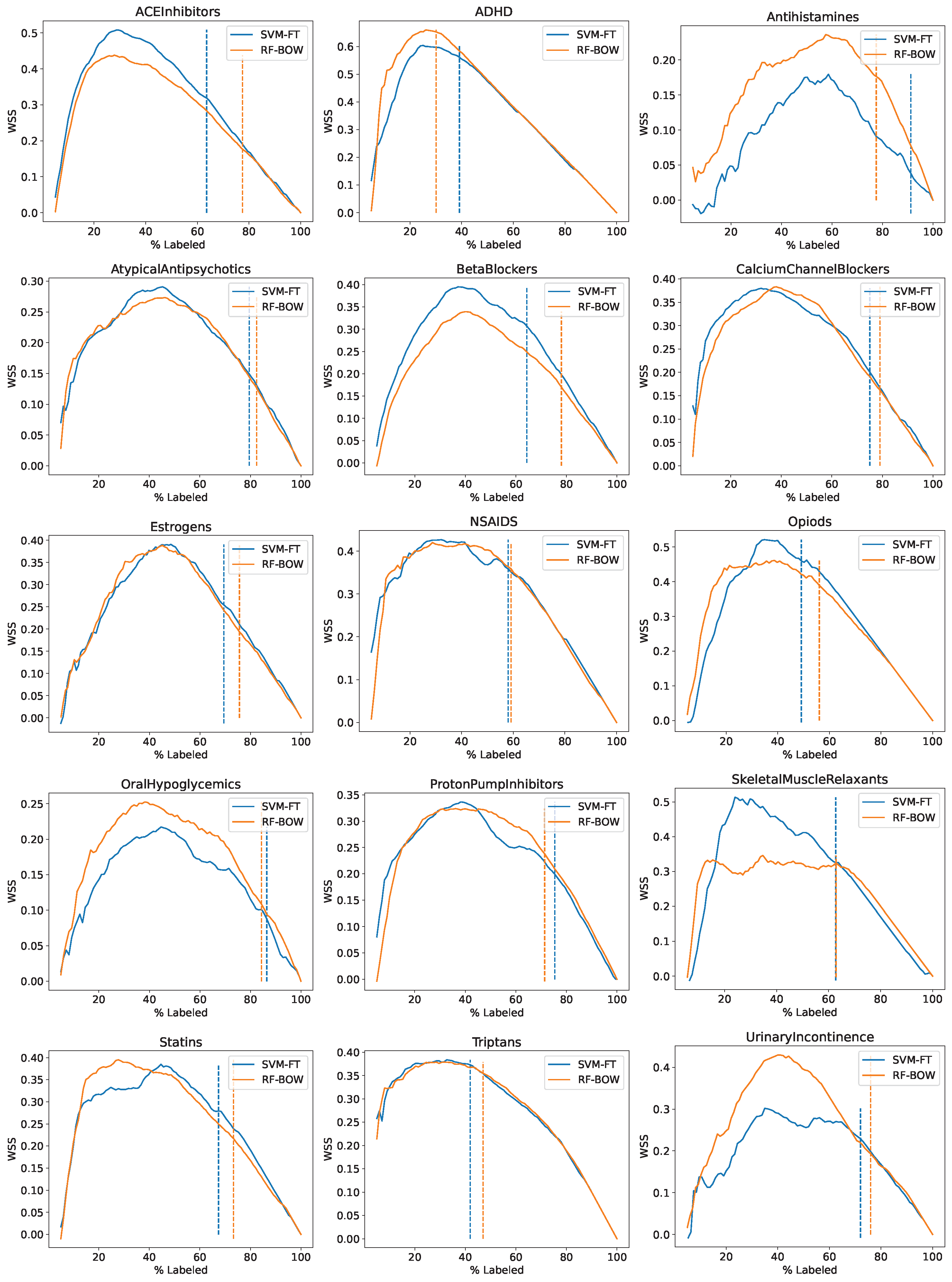
3.8. SLR Workload Reduction
Experiments to estimate the SLR workload reduction using the WSS measure were performed only for the generally most successful active learning setups: the SVM algorithm with the FastText representation and the random forest algorithm with the bag of words representation; both used with random initialization and uncertainty sampling query selection only. Figure 4 presents the obtained learning curves, plotting the WSS value obtained for the default decision threshold of predicted relevant class probability equal versus the percentage of data labeled so far. Vertical dashed lines mark iterations when a recall value of or higher were first achieved. The corresponding WSS@95% values are presented in Table 9.
The following observations can be made.
- The highest workload reduction is typically achieved after labeling 20–40% of articles and ranges from about to about .
- The recall level of is typically achieved after labeling 60–80% of articles, which corresponds to WSS@95% values between and for SVM-FT ( on average) or between and for RF-BOW ( on average).
- With respect to peak WSS values, RF-BOW outperforms SVM-FT for datasets, SVM-FT outperforms RF-BOW for datasets, and they perform similarly to each other for eight datasets.
- With respect to WSS@95%, SVM-FT outperforms RF-BOW for datasets, RF-BOW outperforms SVM-FT for datasets, and they perform similarly to each other (within a margin) for datasets.
Table 10 shows how the WSS@95% values from Table 9 are related to the size and relevant class percentage of particular datasets according to the Spearman rank correlation. Unlike the results previously observed for prediction quality measured using the area under the precision–recall curve, workload reduction is positively correlated with data size (although this effect only occurs for SVM-FT) and negatively correlated with the relevant class percentage. This means that more savings in the SLR process are obtained for datasets that are harder to classify (bigger and more imbalanced). Even though the classification performance for such datasets is worse, they require considerably more human labeling effort, and a greater part thereof can be avoided due to active learning.
3.9. Discussion
The presented results show that active learning can often deliver text classification models with predictive utility approaching that of standard passive learning using between 25% and 50% of the data. In some cases, the passive learning performance level can be even exceeded, i.e., a small subset of appropriately selected training articles may be more useful than the full dataset. However, and not surprisingly, the performance varies across datasets, and achieving substantial savings due to active learning is not possible for all of them. Also, while uncertainty sampling is generally superior to random sampling, it is not always so for each particular dataset.
Two of the four examined combinations of classification algorithms and text representation methods were the most successful: the SVM algorithm with the FastText representation and the random forest algorithm with the bag of words representation. While RF worked nearly as well with the FastText representation, SVM with bag of words turned out clearly the worst of the bunch. It delivered inferior models to those produced by the other algorithm–representation combinations throughout the whole active learning process, with particularly high differences at the beginning, when the training set is small. This is an interesting and potentially useful finding given the fact that such a combination appears to be one of the most popular and widely used setups for text classification with non-neural algorithms, particularly in the active learning scenario. It appears that the relatively high dimensionality of bag of words combined with a low training set size does not provide ideal conditions for a successful SVM application.
While both the uncertainty-based and stability-based early stopping criteria can terminate the active learning process when little or no further improvement is likely, the proper choice of the stopping threshold may depend on the classification algorithm and the text representation method as well as on the dataset. The threshold setup for confidence-based stopping appears to be less dependent on the algorithm–representation combination and the dataset than for stability-based stopping criteria, though.
Since stability-based stopping is based on the correlation between class probability predictions from consecutive active learning iterations, the observed different behavior of these criteria for the SVM and RF algorithms may be related to the fact that they produce probabilistic predictions in a very different way. The probabilistic predictions of SVM are obtained by Platt’s scaling [35] and therefore are usually well calibrated, which may also make them more stable between active learning iterations. The probabilistic predictions of RF, obtained by the voting of individual decision trees, may be not so well calibrated and therefore exhibit more variability between active learning iterations.
The 26–28% average workload reduction possible to obtain in an SLR application may not be spectacular, but it is still with no doubt useful. It is worthwhile to underline that it was estimated in a fully realistic setting. A fixed decision threshold was used without assuming that it can be optimally adjusted for each algorithm setup and dataset, which would not be possible in an actual application. The effort needed to provide class labels for all training articles was included in WSS calculation. This is unlike in the previous passive learning studies, reporting an average workload reduction of 30–40% [24,51,53,62] when using test set predictions, which assumed the availability of training data labels “for free” and the possibility of adjusting the decision threshold to ensure the desired recall level [24,51,53,62]. Even in active learning, SLR research studies on WSS calculation details are not always clear, and in some cases, the labeling effort for the initial training set is excluded. This appears to be the way WSS is calculated by the ASReview system [19].
While this work does not report computational time results, the expense of creating dozens of models during the active learning process is not by any means prohibitive. Even for the full biggest dataset used in this study, creating a single model takes no longer than a few seconds when run on a single CPU core, which would be more than acceptable during an interactive SLR session. The overall time of active learning would be dominated by the time needed for human article screening anyway.
4. Conclusions
The experimental study presented in this article confirms that active learning is a useful approach to create text classification models for SLR studies. It makes it possible to save at least half of the human effort needed to assign relevant or irrelevant class labels to training articles used for model creation without loss of classification quality. It also reduces the systematic literature review workload, by about 25–30% on the average. The standard active learning setup with random initialization and uncertainty sampling query selection works well with the random forest algorithm using the bag of words representation and with the SVM algorithm using the FastText representation.
The above findings were achieved using a reliable -fold cross-validation procedure and the area under the precision–recall curve as the performance measure. With imbalanced datasets, this is a more reliable prediction quality indicator than any single-point measure (such as precision, recall, F-measure etc.) or the area of the ROC curve. To avoid an unrealistic assumption of labeled data being available for hyperparameter tuning and a possible resulting optimistic bias, mostly default algorithm settings are used. The default setup performance is arguably more interesting from a practical point of view than that of a tuned configuration given the fact that tuning is hardly applicable in realistic active learning application scenarios.
Despite the broad scope of the experimental study reported in this article, it leaves some interesting issues postponed for future work. Four continuation directions are particularly noteworthy. First, since the hardness of text classification is often related to class imbalance and it is natural for systematic literature review data to have heavily imbalanced classes, it would make sense to investigate the utility of different imbalance compensation techniques when combined with selected text representation methods and classification algorithms. In the reported experiments, class rebalancing weights were only used, but data resampling approaches, including generating synthetic minority class instances [63,64], might sometimes work better. Second, since active learning is not the only possible approach to saving the human effort needed to provide class labels for classification model creation, it would be interesting to examine the utility of other possible approaches, such as semi-supervised learning [65]—either alone or in combination with active learning. Third, it would be a good idea to revisit the issue of active learning early stopping criteria to make them more reliable and easier to use without tuning by using some adaptive methods of adjusting the threshold parameter or a separate stop set [46]. Last but not least, a more thorough estimation of human work saved in the systematic literature review process is needed before an actual SLR application is developed and deployed based on the algorithms studied in this article. While this work primarily applied machine learning predictive performance evaluation methods to reliably compare different algorithms, text representations, and active learning setups, such an SLR evaluation would provide performance estimates that are more interpretable and useful for SLR practitioners.
Funding
This research received no external funding.
Institutional Review Board Statement
Not applicable.
Informed Consent Statement
Not applicable.
Data Availability Statement
The datasets used for this work, prepared as described in Section 3.1, are available from [66].
Conflicts of Interest
The author declares no conflicts of interest.
References
- McCallum, A.; Nigam, K. A Comparison of Event Models for Naive Bayes Text Classification. In Proceedings of the AAAI/ICML-98 Workshop on Learning for Text Categorization, Menlo Park, CA, USA, 26–27 July 1998. [Google Scholar]
- Joachims, T. Text Categorization with Support Vector Machines: Learning with Many Relevant Features. In Proceedings of the Tenth European Conference on Machine Learning (ECML-1998), Berlin, Germany, 21–23 April 1998. [Google Scholar]
- Radovanović, M.; Ivanović, M. Text Mining: Approaches and Applications. Novi Sad J. Math. 2008, 38, 227–234. [Google Scholar]
- Rousseau, F.; Kiagias, E.; Vazirgiannis, M. Text Categorization as a Graph Classification Problem. In Proceedings of the Fifty-Third Annual Meeting of the Association for Computational Linguistics and the Sixth International Joint Conference on Natural Language Processing (ACL-IJCNLP-2015), Beijing, China, 26–31 July 2015. [Google Scholar]
- Dařena, F.; Žižka, J. Ensembles of Classifiers for Parallel Categorization of Large Number of Text Documents Expressing Opinions. J. Appl. Econ. Sci. 2017, 12, 25–35. [Google Scholar]
- Zymkowski, T.; Szymański, J.; Sobecki, A.; Drozda, P.; Szałapak, K.; Komar-Komarowski, K.; Scherer, R. Short Texts Representations for Legal Domain Classification. In Proceedings of the Twenty-First International Conference on Artificial Intelligence and Soft Computing (ICAISC-2022); Springer: Berlin/Heidelberg, Germany, 2022. [Google Scholar]
- García Adeva, J.J.; Pikatza Atxaa, J.M.; Ubeda Carrillo, M.; Ansuategi Zengotitabengoa, E. Automatic Text Classification to Support Systematic Reviews in Medicine. Expert Syst. Appl. 2014, 41, 1498–1508. [Google Scholar] [CrossRef]
- van den Bulk, L.M.; Bouzembrak, Y.; Gavai, A.; Liu, N.; van den Heuvel, L.J.; Marvin, H.J.P. Automatic Classification of Literature in Systematic Reviews on Food Safety Using Machine Learning. Curr. Res. Food Sci. 2022, 5, 84–95. [Google Scholar] [CrossRef]
- Cohn, D.; Atlas, L.; Ladner, R. Improving Generalization with Active Learning. Mach. Learn. 1994, 15, 201–221. [Google Scholar] [CrossRef]
- Tharwat, A.; Schenck, W. A Survey on Active Learning: State-of-the-Art, Practical Challenges and Research Directions. Mathematics 2023, 11, 820. [Google Scholar] [CrossRef]
- Borisov, V.; Leemann, T.; Seßler, K.; Haug, J.; Pawelczyk, M.; Kasneci, G. Deep Neural Networks and Tabular Data: A Survey. arXiv 2022, arXiv:2110.01889. [Google Scholar] [CrossRef] [PubMed]
- Ren, P.; Xiao, Y.; Chang, X.; Huang, P.Y.; Li, Z.; Gupta, B.B.; Chen, X.; Wang, X. A Survey of Deep Active Learning. ACM Comput. Surv. 2020, 54, 180. [Google Scholar] [CrossRef]
- Cichosz, P. Bag of Words and Embedding Text Representation Methods for Medical Article Classification. Int. J. Appl. Math. Comput. Sci. 2023, 33, 603–621. [Google Scholar] [CrossRef]
- Tong, S.; Koller, D. Support Vector Machine Active Learning with Applications to Text Classification. J. Mach. Learn. Res. 2001, 2, 45–66. [Google Scholar]
- Zhu, J.; Wang, H.; Yao, T.; Tsou, B.K. Active Learning with Sampling by Uncertainty and Density for Word Sense Disambiguation and Text Classification. In Proceedings of the Twenty-Second International Conference on Computational Linguistics (COLING-2008), Stroudsburg, PA, USA, 18–22 August 2008. [Google Scholar]
- Miwa, M.; Thomas, J.; O’Mara-Eves, A.; Ananiadou, S. Reducing Systematic Review Workload through Certainty-Based Screening. J. Biomed. Inform. 2014, 51, 242–253. [Google Scholar] [CrossRef] [PubMed]
- Goudjil, M.; Koudil, M.; Bedda, M.; Ghoggali, N. A Novel Active Learning Method Using SVM for Text Classification. Int. J. Autom. Comput. 2018, 15, 290–298. [Google Scholar] [CrossRef]
- Flores, C.A.; Figueroa, R.L.; Pezoa, J.E. Active Learning for Biomedical Text Classification Based on Automatically Generated Regular Expressions. IEEE Access 2021, 9, 38767–38777. [Google Scholar] [CrossRef]
- van de Schoot, R.; de Bruin, J.; Schram, R.; Zahedi, P.; de Boer, J.; Weijdema, F.; Kramer, B.; Huijts, M.; Hoogerwerf, M.; Ferdinands, G.; et al. An Open Source Machine Learning Framework for Efficient and Transparent Systematic Reviews. Nat. Mach. Intell. 2021, 3, 125–133. [Google Scholar] [CrossRef]
- Miller, B.; Linder, F.; Mebane, W.R. Active Learning Approaches for Labeling Text: Review and Assessment of the Performance of Active Learning Approaches. Political Anal. 2020, 28, 532–551. [Google Scholar] [CrossRef]
- Jacobs, P.F.; Maillette de Buy Wenniger, G.; Wiering, M.; Schomaker, L. Active Learning for Reducing Labeling Effort in Text Classification Tasks. In Proceedings of the Artificial Intelligence and Machine Learning: Proceedings of the Thirty-Third Benelux on Artificial Intelligence (BNAIC/Benelearn-2021), Cham, Switzerland, 10–12 November 2021. [Google Scholar]
- Ferdinands, G.; Schram, R.; de Bruin, J.; Bagheri, A.; Oberski, D.L.; Tummers, L.; Teijema, J.J.; van de Schoot, R. Performance of Active Learning Models for Screening Prioritization in Systematic Reviews: A Simulation Study into the Average Time to Discover Relevant Record. Syst. Rev. 2023, 12, 100. [Google Scholar] [CrossRef]
- Teijema, J.J.; Hofstee, L.; Brouwer, M.; de Bruin, J.; Ferdinands, G.; de Boer, J.; Vizan, P.; van den Brand, S.; Bockting, C.; van de Schoot, R.; et al. Active Learning-Based Systematic Reviewing Using Switching Classification Models: The Case of the Onset, Maintenance, and Relapse of Depressive Disorders. Front. Res. Metrics Anal. 2023, 8, 1178181. [Google Scholar] [CrossRef]
- Cohen, A.M.; Hersh, W.R.; Peterson, K.; Yen, P.Y. Reducing Workload in Systematic Review Preparation Using Automated Citation Classification. J. Am. Med. Inform. Assoc. 2006, 13, 206–219. [Google Scholar] [CrossRef]
- Breiman, L. Random Forests. Mach. Learn. 2001, 45, 5–32. [Google Scholar] [CrossRef]
- Cortes, C.; Vapnik, V.N. Support-Vector Networks. Mach. Learn. 1995, 20, 273–297. [Google Scholar] [CrossRef]
- Aggarwal, C.C.; Zhai, C.X. (Eds.) Mining Text Data; Springer: New York, NY, USA, 2012. [Google Scholar]
- Bojanowski, P.; Grave, E.; Joulin, A.; Mikolov, T. Enriching Word Vectors with Subword Information. arXiv 2016, arXiv:1607.04606. [Google Scholar] [CrossRef]
- Dumais, S.T.; Platt, J.C.; Heckerman, D.; Sahami, M. Inductive Learning Algorithms and Representations for Text Categorization. In Proceedings of the Seventh International Conference on Information and Knowledge Management (CIKM-98), Bethesda, MD, USA, 2–7 November 1998; pp. 148–155. [Google Scholar]
- Szymański, J. Comparative Analysis of Text Representation Methods Using Classification. Cybern. Syst. 2014, 45, 180–199. [Google Scholar] [CrossRef]
- Salton, G.; Buckley, C. Term Weighting Approaches in Automatic Text Retrieval. Inf. Process. Manag. 1988, 24, 513–523. [Google Scholar] [CrossRef]
- Mikolov, T.; Chen, K.; Corrado, G.S.; Dean, J. Efficient Estimation of Word Representations in Vector Space. arXiv 2013, arXiv:1301.3781. [Google Scholar]
- Platt, J.C. Fast Training of Support Vector Machines using Sequential Minimal Optimization. In Advances in Kernel Methods: Support Vector Learning; Schölkopf, B., Burges, C.J.C., Smola, A.J., Eds.; MIT Press: Cambridge, MA, USA, 1998. [Google Scholar]
- Hamel, L.H. Knowledge Discovery with Support Vector Machines; Wiley: Hoboken, NJ, USA, 2009. [Google Scholar]
- Platt, J.C. Probabilistic Outputs for Support Vector Machines and Comparison to Regularized Likelihood Methods. In Advances in Large Margin Classifiers; Smola, A.J., Barlett, P., Schölkopf, B., Schuurmans, D., Eds.; MIT Press: Cambridge, MA, USA, 2000. [Google Scholar]
- Rios, G.; Zha, H. Exploring Support Vector Machines and Random Forests for Spam Detection. In Proceedings of the First International Conference on Email and Anti Spam (CEAS-2004), Mountain View, CA, USA, 30–31 July 2004. [Google Scholar]
- Breiman, L. Bagging Predictors. Mach. Learn. 1996, 24, 123–140. [Google Scholar] [CrossRef]
- Koprinska, I.; Poon, J.; Clark, J.; Chan, J. Learning to Classify E-Mail. Inf. Sci. Int. J. 2007, 177, 2167–2187. [Google Scholar] [CrossRef]
- Xue, D.; Li, F. Research of Text Categorization Model Based on Random Forests. In Proceedings of the 2015 IEEE International Conference on Computational Intelligence and Communication Technology (CICT-2015), Los Alamitos, CA, USA, 13–14 February 2015. [Google Scholar]
- Cichosz, P. A Case Study in Text Mining of Discussion Forum Posts: Classification with Bag of Words and Global Vectors. Int. J. Appl. Math. Comput. Sci. 2018, 28, 787–801. [Google Scholar] [CrossRef]
- Yuan, W.; Han, Y.; Guan, D.; Lee, S.; Lee, Y.K. Initial Training Data Selection for Active Learning. In Proceedings of the Fifth International Conference on Ubiquitous Information Management and Communication (ICUIMC-2011), Seoul, Republic of Korea, 21–23 February 2011. [Google Scholar]
- Bezdek, J.C. Pattern Recognition with Fuzzy Objective Function Algorithms; Springer: New York, NY, USA, 1981. [Google Scholar]
- Jolliffe, I.T. Pricipal Component Analysis; Springer: Berlin/Heidelberg, Germany, 2002. [Google Scholar]
- Fu, Y.; Zhu, X.; Li, B. A Survey on Instance Selection for Active Learning. Knowl. Inf. Syst. 2013, 35, 249–283. [Google Scholar] [CrossRef]
- Nguyen, V.; Shaker, M.H.; Hüllermeier, E. How to Measure Uncertainty in Uncertainty Sampling for Active Learning. Mach. Learn. 2022, 111, 89–122. [Google Scholar] [CrossRef]
- Kurlandski, L.; Bloodgood, M. Impact of Stop Sets on Stopping Active Learning for Text Classification. In Proceedings of the Sixteenth International Conference on Semantic Computing (ICSC-2022), Los Alamitos, CA, USA, 26–28 January 2022. [Google Scholar]
- Zhu, J.; Wang, H.; Hovy, E.; Ma, M. Confidence-Based Stopping Criteria for Active Learning for Data Annotation. ACM Trans. Speech Lang. Process. 2010, 6, 3. [Google Scholar] [CrossRef]
- Bloodgood, M.; Vijay-Shanker, K. A Method for Stopping Active Learning Based on Stabilizing Predictions and the Need for User-Adjustable Stopping. In Proceedings of the Thirteenth Conference on Computational Natural Language Learning (CoNLL-2009). Association for Computational Linguistics, Boulder, CO, USA, 4–5 June 2009. [Google Scholar]
- Systematic Drug Class Review Gold Standard Data. Available online: https://dmice.ohsu.edu/cohenaa/systematic-drug-class-review-data.html (accessed on 1 July 2024).
- Cohen, A.M. Optimizing Feature Representation for Automated Systematic Review Work Prioritization. In Proceedings of the AMIA Annual Symposium Proceedings, AMIA, Washington, DC, USA, 8–12 November 2008; pp. 121–125. [Google Scholar]
- Matwin, S.; Kouznetsov, A.; Inkpen, D.; Frunza, O.; O’Blenis, P. A New Algorithm for Reducing the Workload of Experts in Performing Systematic Reviews. J. Am. Med. Inform. Assoc. 2010, 17, 446–453. [Google Scholar] [CrossRef] [PubMed]
- Jonnalagadda, S.; Petitti, D. A New Iterative Method to Reduce Workload in Systematic Review Process. Int. J. Comput. Biol. Drug Des. 2013, 6, 5–17. [Google Scholar] [CrossRef]
- Khabsa, M.; Elmagarmid, A.; Ilyas, I.; Hammady, H.; Ouzzani, M. Learning to Identify Relevant Studies for Systematic Reviews Using Random Forest and External Information. Mach. Learn. 2016, 102, 465–482. [Google Scholar] [CrossRef]
- Ji, X.; Ritter, A.; Yen, P.Y. Using Ontology-Based Semantic Similarity to Facilitate the Article Screening Process for Systematic Reviews. J. Biomed. Inform. 2017, 69, 33–42. [Google Scholar] [CrossRef]
- Pedregosa, F.; Varoquaux, G.; Gramfort, A.; Michel, V.; Thirion, B.; Grisel, O.; Blondel, M.; Prettenhofer, P.; Weiss, R.; Dubourg, V.; et al. Scikit-learn: Machine Learning in Python. J. Mach. Learn. Res. 2011, 12, 2825–2830, Library version 1.1.3. [Google Scholar]
- Honnibal, M.; Montani, I.; Van Landeghem, S.; Boyd, A. spaCy: Industrial-Strength Natural Language Processing in Python. Library version 3.3.1. 2022. Available online: https://github.com/explosion/spaCy/blob/master/CITATION.cff (accessed on 1 July 2024).
- Bojanowski, P.; Grave, E.; Joulin, A.; Mikolov, T. fastText: Library for Efficient Text Classification and Representation Learning. Library version 0.9.2. 2020. Available online: https://fasttext.cc/ (accessed on 1 July 2024).
- Egan, J.P. Signal Detection Theory and ROC Analysis; Academic Press: New York, NY, USA, 1975. [Google Scholar]
- Fawcett, T. An Introduction to ROC Analysis. Pattern Recognit. Lett. 2006, 27, 861–874. [Google Scholar] [CrossRef]
- Arlot, S.; Celisse, A. A Survey of Cross-Validation Procedures for Model Selection. Stat. Surv. 2010, 4, 40–79. [Google Scholar] [CrossRef]
- Wallace, B.C.; Trikalinos, T.A.; Lau, J.; Brodley, C.; Schmid, C.H. Semi-Automated Screening of Biomedical Citations for Systematic Reviews. BMC Bioinform. 2010, 11, 55. [Google Scholar] [CrossRef]
- Cohen, A.M. Performance of Support-Vector-Machine-Based Classification on 15 Systematic Review Topics Evaluated with the WSS@95 Measure. J. Am. Med. Inform. Assoc. 2011, 18, 104. [Google Scholar] [CrossRef]
- Chawla, N.V.; Bowyer, K.W.; Hall, L.O.; Kegelmeyer, W.P. SMOTE: Synthetic Minority Over-sampling Technique. J. Artif. Intell. Res. 2002, 16, 321–357. [Google Scholar] [CrossRef]
- Menardi, G.; Torelli, N. Training and Assessing Classification Rules with Imbalanced Data. Data Min. Knowl. Discov. 2014, 28, 92–122. [Google Scholar] [CrossRef]
- Zhu, X.; Goldberg, A. Introduction to Semi-Supervised Learning; Morgan & Claypool: San Rafael, CA, USA, 2009. [Google Scholar]
- Text Classification Data from 15 Drug Class Review SLR Studies. Available online: https://figshare.com/articles/dataset/Text_Classification_Data_from_15_Drug_Class_Review_SLR_Studies/23626656/1?file=41457282 (accessed on 1 July 2024).
Figure 1.
Learning curves for SVM-FT and RF-BOW with random initialization and uncertainty sampling.
Figure 1.
Learning curves for SVM-FT and RF-BOW with random initialization and uncertainty sampling.
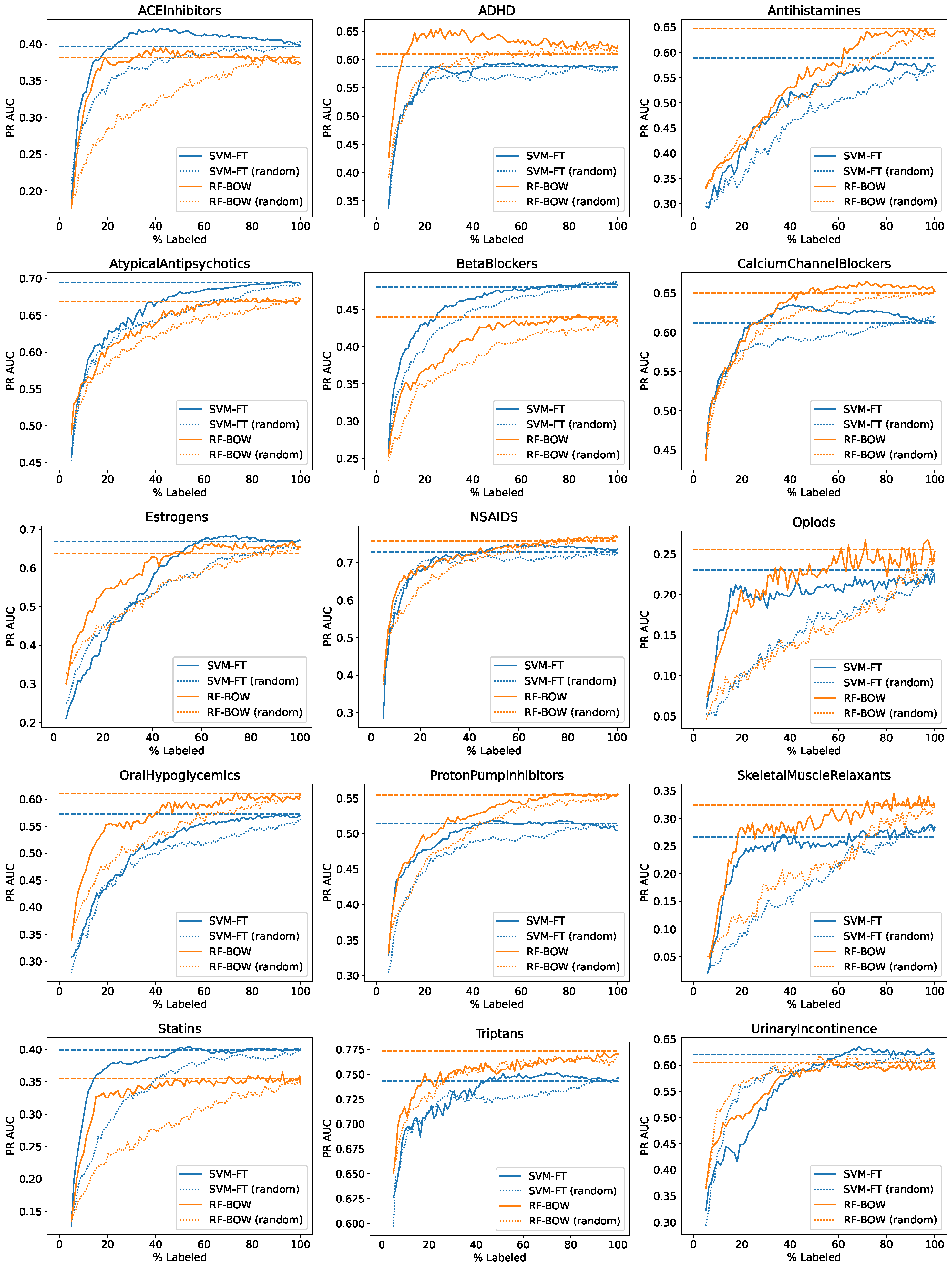
Figure 2.
Learning curves with confidence-based stopping criteria marks for SVM-FT and RF-BOW with random initialization and uncertainty sampling.
Figure 2.
Learning curves with confidence-based stopping criteria marks for SVM-FT and RF-BOW with random initialization and uncertainty sampling.
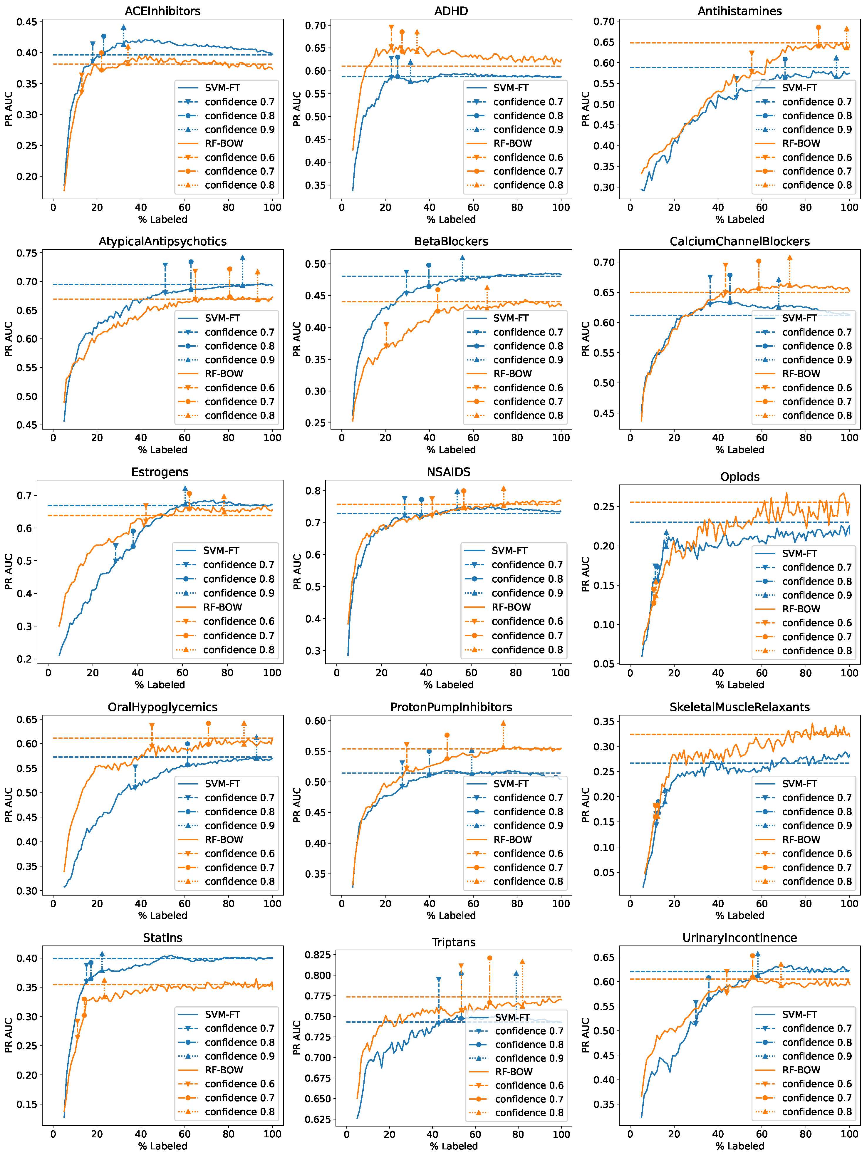
Figure 3.
Learning curves with stability-based stopping criteria marks for SVM-FT and RF-BOW with random initialization and uncertainty sampling.
Figure 3.
Learning curves with stability-based stopping criteria marks for SVM-FT and RF-BOW with random initialization and uncertainty sampling.
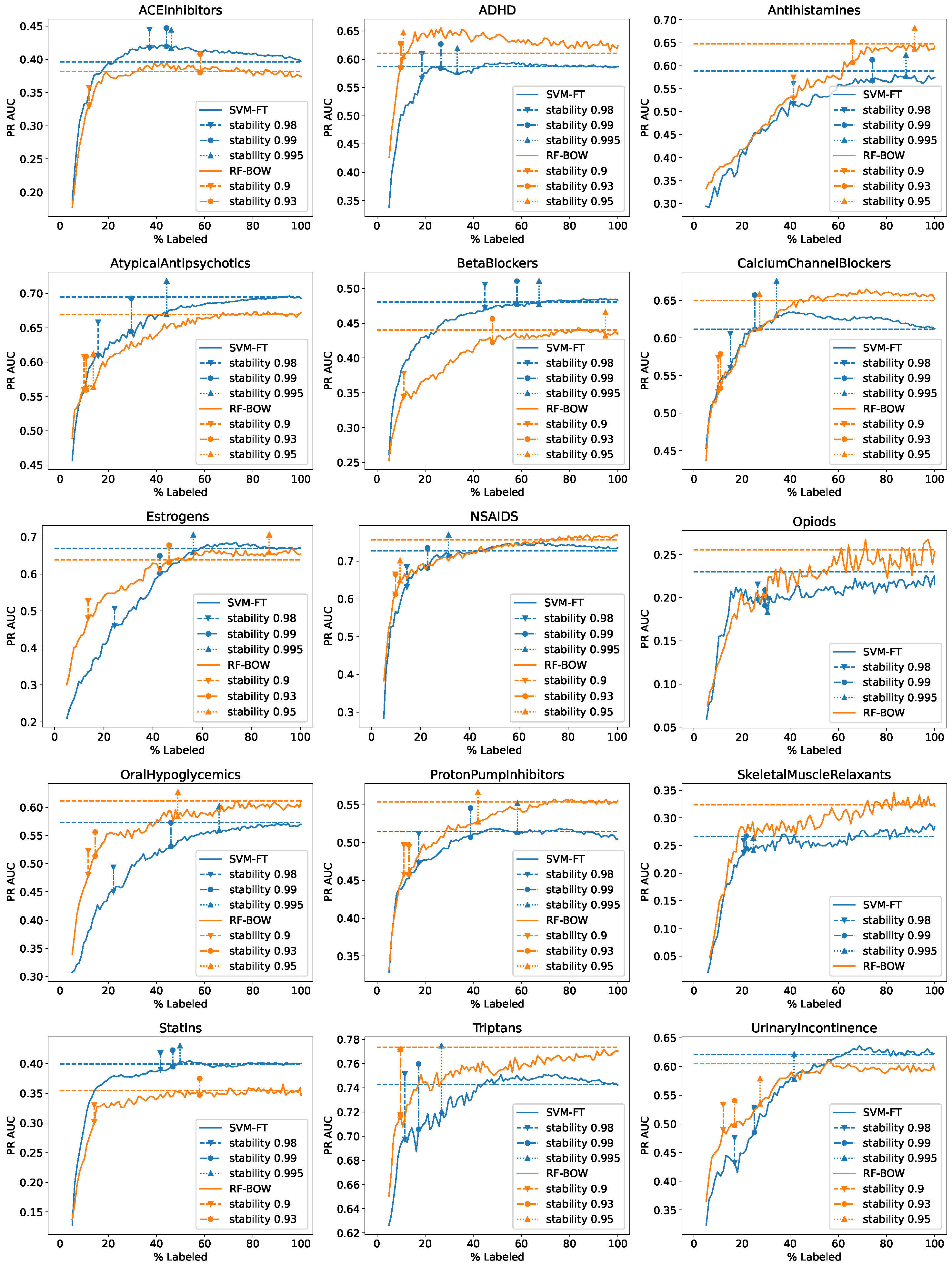
Figure 4.
WSS learning curves for SVM-FT and RF-BOW with uncertainty sampling.

Table 1.
Related work.
| Ref. | Representations | Algorithms | AL Setups | Evaluation | Data |
|---|---|---|---|---|---|
| [14] | BOW (TF-IDF) | SVM | initialization: random; query: margin; stopping: none | error, precision–recall breakeven; train–test split | Reuters, subset of Newsgroups |
| [15] | BOW | maxent | initialization: cluster; query: uncertainty; stopping: none | accuracy; k-fold CV | subset of Newsgroups, WebKB |
| [16] | BOW, LDA | SVM | initialization: unknown, query: uncertainty, minority, committee; stopping: none | utility, coverage, ROC AUC; train–test split, train+pool evaluation | 3 medical and 4 social science SLR studies |
| [17] | BOW (TF-IDF) | SVM | initialization: random; query: uncertainty (custom); stopping: none | accuracy; train–test split | Reuters, Newsgroups, WebKB |
| [18] | BOW (1- and 2-gram) | regex classifier, NB, SVM, BERT | initialization: random; query: uncertainty (custom); stopping: query score variance | accuracy, precision F1; k-fold CV | 3 biomedical datasets |
| [19] | BOW (TF-IDF) | NB | initialization: random; query: minority; stopping: none | WSS, RRF; train+pool evaluation | 2 biomedical SLR studies, 1 software fault prediction SLR study, 1 longitudinal SLR study |
| [20] | BOW | SVM, NB, LR | initialization: random; query: margin, committee; stopping: none | F1; train–test split | Twitter (refugee topic), Wikipedia talk pages (toxic comments), Breibart news |
| [21] | — | BERT | initialization: random; query: uncertainty (custom); stopping: none | accuracy; train–test split | Stanford Sentiment Treeban, KvK-Frontpages |
| [22] | BOW (TF-IDF), doc2vec | SVM, NB, LR, RF | initialization: random; query: minority; stopping: none | WSS, RRF, TD; train+pool evaluation | 6 biomedical SLR studies |
| [23] | BOW (TF-IDF), sBERT | CNN, SVM, RF, LR, NB | initialization: random; query: minority; stopping: none | WSS, TD, recall; train+pool evaluation | 1 biomedical SLR study |
Table 2.
Dataset sizes and class distribution.
| Dataset | Size | Relevant % |
|---|---|---|
| ACEInhibitors | 2215 | 7.54 |
| ADHD | 797 | 10.41 |
| Antihistamines | 285 | 31.23 |
| AtypicalAntipsychotics | 1020 | 32.45 |
| BetaBlockers | 1849 | 14.49 |
| CalciumChannelBlockers | 1100 | 23.18 |
| Estrogens | 344 | 22.67 |
| NSAIDS | 355 | 23.38 |
| Opiods | 1760 | 2.44 |
| OralHypoglycemics | 466 | 28.11 |
| ProtonPumpInhibitors | 1193 | 18.69 |
| SkeletalMuscleRelaxants | 1341 | 2.24 |
| Statins | 2727 | 5.50 |
| Triptans | 585 | 34.36 |
| UrinaryIncontinence | 283 | 24.03 |
Table 3.
Average PR AUC values obtained for random initialization.
| (a) uncertainty sampling | (b) diversity sampling | ||||||||
| SVM-BOW | SVM-FT | RF-BOW | RF-FT | SVM-BOW | SVM-FT | RF-BOW | RF-FT | ||
| 5% | 0.19 | 0.29 | 0.32 | 0.32 | 5% | 0.19 | 0.29 | 0.32 | 0.32 |
| 10% | 0.27 | 0.40 | 0.42 | 0.40 | 10% | 0.24 | 0.34 | 0.35 | 0.36 |
| 25% | 0.36 | 0.48 | 0.50 | 0.48 | 25% | 0.30 | 0.40 | 0.40 | 0.41 |
| 33% | 0.39 | 0.50 | 0.51 | 0.50 | 33% | 0.34 | 0.43 | 0.43 | 0.43 |
| 50% | 0.44 | 0.53 | 0.54 | 0.52 | 50% | 0.40 | 0.48 | 0.47 | 0.47 |
| 66% | 0.47 | 0.54 | 0.54 | 0.53 | 66% | 0.43 | 0.50 | 0.50 | 0.50 |
| 75% | 0.48 | 0.54 | 0.55 | 0.53 | 75% | 0.45 | 0.52 | 0.51 | 0.51 |
| 100% | 0.49 | 0.54 | 0.55 | 0.53 | 100% | 0.49 | 0.54 | 0.55 | 0.53 |
| (c) minority sampling | (d) threshold sampling | ||||||||
| SVM-BOW | SVM-FT | RF-BOW | RF-FT | SVM-BOW | SVM-FT | RF-BOW | RF-FT | ||
| 5% | 0.19 | 0.29 | 0.32 | 0.32 | 5% | 0.19 | 0.29 | 0.31 | 0.33 |
| 10% | 0.27 | 0.39 | 0.41 | 0.39 | 10% | 0.26 | 0.38 | 0.42 | 0.41 |
| 25% | 0.35 | 0.46 | 0.49 | 0.48 | 25% | 0.36 | 0.48 | 0.49 | 0.48 |
| 33% | 0.39 | 0.49 | 0.51 | 0.50 | 33% | 0.39 | 0.49 | 0.51 | 0.50 |
| 50% | 0.44 | 0.53 | 0.53 | 0.53 | 50% | 0.43 | 0.52 | 0.53 | 0.52 |
| 66% | 0.46 | 0.54 | 0.55 | 0.53 | 66% | 0.46 | 0.53 | 0.54 | 0.53 |
| 75% | 0.47 | 0.54 | 0.55 | 0.53 | 75% | 0.47 | 0.53 | 0.55 | 0.53 |
| 100% | 0.49 | 0.54 | 0.55 | 0.53 | 100% | 0.49 | 0.54 | 0.55 | 0.53 |
| (e) random sampling | |||||||||
| SVM-BOW | SVM-FT | RF-BOW | RF-FT | ||||||
| 5% | 0.19 | 0.29 | 0.32 | 0.33 | |||||
| 10% | 0.25 | 0.37 | 0.38 | 0.38 | |||||
| 25% | 0.37 | 0.46 | 0.45 | 0.45 | |||||
| 33% | 0.39 | 0.48 | 0.47 | 0.47 | |||||
| 50% | 0.43 | 0.50 | 0.50 | 0.49 | |||||
| 66% | 0.46 | 0.51 | 0.52 | 0.51 | |||||
| 75% | 0.47 | 0.52 | 0.53 | 0.52 | |||||
| 100% | 0.49 | 0.54 | 0.55 | 0.53 | |||||
Table 4.
Average PR AUC values for cluster initialization.
| (a) uncertainty sampling | (b) diversity sampling | ||||||||
| SVM-BOW | SVM-FT | RF-BOW | RF-FT | SVM-BOW | SVM-FT | RF-BOW | RF-FT | ||
| 5% | 0.19 | 0.28 | 0.33 | 0.33 | 5% | 0.19 | 0.30 | 0.33 | 0.33 |
| 10% | 0.27 | 0.40 | 0.43 | 0.41 | 10% | 0.24 | 0.35 | 0.36 | 0.36 |
| 25% | 0.38 | 0.49 | 0.50 | 0.49 | 25% | 0.31 | 0.42 | 0.41 | 0.41 |
| 33% | 0.40 | 0.51 | 0.52 | 0.50 | 33% | 0.34 | 0.45 | 0.43 | 0.43 |
| 50% | 0.45 | 0.53 | 0.53 | 0.53 | 50% | 0.40 | 0.48 | 0.47 | 0.47 |
| 66% | 0.47 | 0.53 | 0.54 | 0.53 | 66% | 0.43 | 0.51 | 0.49 | 0.49 |
| 75% | 0.48 | 0.54 | 0.54 | 0.53 | 75% | 0.45 | 0.52 | 0.51 | 0.51 |
| 100% | 0.49 | 0.54 | 0.55 | 0.53 | 100% | 0.49 | 0.54 | 0.55 | 0.53 |
| (c) minority sampling | (d) threshold sampling | ||||||||
| SVM-BOW | SVM-FT | RF-BOW | RF-FT | SVM-BOW | SVM-FT | RF-BOW | RF-FT | ||
| 5% | 0.19 | 0.29 | 0.33 | 0.34 | 5% | 0.19 | 0.28 | 0.33 | 0.33 |
| 10% | 0.28 | 0.40 | 0.42 | 0.39 | 10% | 0.26 | 0.38 | 0.44 | 0.41 |
| 25% | 0.36 | 0.48 | 0.49 | 0.48 | 25% | 0.37 | 0.48 | 0.50 | 0.48 |
| 33% | 0.40 | 0.50 | 0.51 | 0.50 | 33% | 0.40 | 0.50 | 0.51 | 0.50 |
| 50% | 0.44 | 0.53 | 0.53 | 0.53 | 50% | 0.44 | 0.52 | 0.52 | 0.52 |
| 66% | 0.47 | 0.54 | 0.54 | 0.53 | 66% | 0.47 | 0.53 | 0.54 | 0.52 |
| 75% | 0.48 | 0.54 | 0.55 | 0.53 | 75% | 0.48 | 0.53 | 0.54 | 0.52 |
| 100% | 0.49 | 0.54 | 0.55 | 0.53 | 100% | 0.49 | 0.54 | 0.55 | 0.53 |
| (e) random sampling | |||||||||
| SVM-BOW | SVM-FT | RF-BOW | RF-FT | ||||||
| 5% | 0.19 | 0.29 | 0.33 | 0.33 | |||||
| 10% | 0.25 | 0.37 | 0.38 | 0.39 | |||||
| 25% | 0.37 | 0.45 | 0.46 | 0.45 | |||||
| 33% | 0.40 | 0.47 | 0.47 | 0.47 | |||||
| 50% | 0.44 | 0.50 | 0.50 | 0.49 | |||||
| 66% | 0.47 | 0.52 | 0.52 | 0.51 | |||||
| 75% | 0.47 | 0.52 | 0.53 | 0.52 | |||||
| 100% | 0.49 | 0.54 | 0.55 | 0.53 | |||||
Table 5.
Rank correlations of PR AUC values at 33% of labeled data to data size and relevant class percentage.
Table 5.
Rank correlations of PR AUC values at 33% of labeled data to data size and relevant class percentage.
| (a) size | ||||
| SVM-BOW | SVM-FT | RF-BOW | RF-FT | |
| random–uncertainty | −0.47 | −0.59 | −0.60 | −0.58 |
| random–diversity | −0.47 | −0.59 | −0.60 | −0.65 |
| random–minority | −0.46 | −0.52 | −0.57 | −0.65 |
| random–threshold | −0.49 | −0.64 | −0.68 | −0.65 |
| random–random | −0.46 | −0.60 | −0.61 | −0.62 |
| cluster–uncertainty | −0.45 | −0.59 | −0.58 | −0.61 |
| cluster–diversity | −0.48 | −0.59 | −0.62 | −0.66 |
| cluster–minority | −0.49 | −0.52 | −0.58 | −0.60 |
| cluster–threshold | −0.40 | −0.63 | −0.66 | −0.60 |
| cluster–random | −0.50 | −0.60 | −0.59 | −0.64 |
| (b) relevant % | ||||
| SVM-BOW | SVM-FT | RF-BOW | RF-FT | |
| random–uncertainty | 0.74 | 0.78 | 0.71 | 0.78 |
| random–diversity | 0.77 | 0.82 | 0.75 | 0.83 |
| random–minority | 0.77 | 0.75 | 0.71 | 0.77 |
| random–threshold | 0.73 | 0.79 | 0.74 | 0.78 |
| random–random | 0.71 | 0.77 | 0.80 | 0.80 |
| cluster–uncertainty | 0.74 | 0.78 | 0.69 | 0.84 |
| cluster–diversity | 0.75 | 0.84 | 0.75 | 0.87 |
| cluster–minority | 0.77 | 0.75 | 0.69 | 0.80 |
| cluster–threshold | 0.60 | 0.76 | 0.75 | 0.77 |
| cluster–random | 0.74 | 0.77 | 0.76 | 0.84 |
Table 6.
PR AUC difference to random sampling at 33% of labeled data.
| (a) smaller | ||||
| SVM-BOW | SVM-FT | RF-BOW | RF-FT | |
| uncertainty | 0.00 | 0.01 | 0.03 | 0.02 |
| diversity | −0.06 | −0.04 | −0.04 | −0.03 |
| minority | −0.01 | 0.00 | 0.02 | 0.02 |
| threshold | 0.00 | 0.01 | 0.02 | 0.02 |
| (b) bigger | ||||
| SVM-BOW | SVM-FT | RF-BOW | RF-FT | |
| uncertainty | 0.01 | 0.06 | 0.06 | 0.04 |
| diversity | −0.05 | −0.04 | −0.04 | −0.04 |
| minority | 0.01 | 0.05 | 0.06 | 0.05 |
| threshold | 0.00 | 0.04 | 0.06 | 0.04 |
| (c) less imbalanced | ||||
| SVM-BOW | SVM-FT | RF-BOW | RF-FT | |
| uncertainty | −0.01 | 0.02 | 0.01 | 0.02 |
| diversity | −0.05 | −0.02 | −0.04 | −0.03 |
| minority | −0.01 | 0.00 | 0.01 | 0.01 |
| threshold | −0.01 | 0.00 | 0.01 | 0.01 |
| (d) more imbalanced | ||||
| SVM-BOW | SVM-FT | RF-BOW | RF-FT | |
| uncertainty | 0.01 | 0.05 | 0.07 | 0.05 |
| diversity | −0.05 | −0.05 | −0.04 | −0.04 |
| minority | 0.01 | 0.05 | 0.07 | 0.06 |
| threshold | 0.01 | 0.03 | 0.06 | 0.05 |
Table 7.
Percentage of the pool used for training when different early stopping criteria were satisfied, averaged over all datasets.
Table 7.
Percentage of the pool used for training when different early stopping criteria were satisfied, averaged over all datasets.
| SVM-BOW | SVM-FT | RF-BOW | RF-FT | |
|---|---|---|---|---|
| confidence 0.5 | 10% | 10% | 10% | 10% |
| confidence 0.6 | 19% | 23% | 34% | 29% |
| confidence 0.7 | 26% | 30% | 48% | 40% |
| confidence 0.8 | 36% | 38% | 61% | 54% |
| confidence 0.9 | 54% | 55% | 77% | 72% |
| confidence 0.95 | 73% | 71% | 89% | 84% |
| confidence 0.98 | 85% | 83% | 98% | 95% |
| stability 0.9 | 14% | 12% | 25% | 28% |
| stability 0.93 | 17% | 13% | 38% | 44% |
| stability 0.95 | 21% | 15% | 58% | 54% |
| stability 0.98 | 43% | 25% | 93% | 87% |
| stability 0.99 | 64% | 37% | 97% | 95% |
| stability 0.995 | 76% | 47% | 100% | 97% |
| stability 0.998 | 84% | 56% | 100% | 100% |
Table 8.
PR AUC values when different early stopping criteria were satisfied, averaged over all datasets.
Table 8.
PR AUC values when different early stopping criteria were satisfied, averaged over all datasets.
| SVM-BOW | SVM-FT | RF-BOW | RF-FT | |
|---|---|---|---|---|
| confidence 0.5 | 0.27 | 0.40 | 0.42 | 0.40 |
| confidence 0.6 | 0.34 | 0.48 | 0.52 | 0.49 |
| confidence 0.7 | 0.37 | 0.50 | 0.54 | 0.51 |
| confidence 0.8 | 0.40 | 0.51 | 0.54 | 0.53 |
| confidence 0.9 | 0.45 | 0.53 | 0.55 | 0.53 |
| confidence 0.95 | 0.47 | 0.54 | 0.55 | 0.53 |
| confidence 0.98 | 0.48 | 0.54 | 0.55 | 0.53 |
| stability 0.9 | 0.30 | 0.42 | 0.50 | 0.49 |
| stability 0.93 | 0.32 | 0.43 | 0.52 | 0.52 |
| stability 0.95 | 0.35 | 0.44 | 0.54 | 0.53 |
| stability 0.98 | 0.42 | 0.48 | 0.55 | 0.53 |
| stability 0.99 | 0.46 | 0.51 | 0.55 | 0.53 |
| stability 0.995 | 0.48 | 0.53 | 0.55 | 0.53 |
| stability 0.998 | 0.48 | 0.53 | 0.55 | 0.53 |
Table 9.
WSS@95% values for SVM-FT and RF-BOW.
| SVM-FT | RF-BOW | |
|---|---|---|
| ACEInhibitors | 0.32 | 0.18 |
| ADHD | 0.56 | 0.65 |
| Antihistamines | 0.04 | 0.18 |
| AtypicalAntipsychotics | 0.15 | 0.13 |
| BetaBlockers | 0.31 | 0.17 |
| CalciumChannelBlockers | 0.20 | 0.16 |
| Estrogens | 0.25 | 0.19 |
| NSAIDS | 0.36 | 0.36 |
| Opiods | 0.46 | 0.39 |
| OralHypoglycemics | 0.09 | 0.11 |
| ProtonPumpInhibitors | 0.20 | 0.24 |
| SkeletalMuscleRelaxants | 0.33 | 0.32 |
| Statins | 0.28 | 0.22 |
| Triptans | 0.37 | 0.35 |
| UrinaryIncontinence | 0.23 | 0.19 |
| AVERAGE | 0.28 | 0.26 |
Table 10.
Rank correlations of WSS@95% values for SVM-FT and RF-BOW to data size and relevant class percentage.
Table 10.
Rank correlations of WSS@95% values for SVM-FT and RF-BOW to data size and relevant class percentage.
| Size | Relevant % | |
|---|---|---|
| SVM-FT | 0.31 | −0.50 |
| RF-BOW | 0.04 | −0.40 |
Disclaimer/Publisher’s Note: The statements, opinions and data contained in all publications are solely those of the individual author(s) and contributor(s) and not of MDPI and/or the editor(s). MDPI and/or the editor(s) disclaim responsibility for any injury to people or property resulting from any ideas, methods, instructions or products referred to in the content. |
© 2024 by the author. Licensee MDPI, Basel, Switzerland. This article is an open access article distributed under the terms and conditions of the Creative Commons Attribution (CC BY) license (https://creativecommons.org/licenses/by/4.0/).
Share and Cite
MDPI and ACS Style
Cichosz, P. Active Learning for Biomedical Article Classification with Bag of Words and FastText Embeddings. Appl. Sci. 2024, 14, 7945. https://doi.org/10.3390/app14177945
AMA Style
Cichosz P. Active Learning for Biomedical Article Classification with Bag of Words and FastText Embeddings. Applied Sciences. 2024; 14(17):7945. https://doi.org/10.3390/app14177945
Chicago/Turabian StyleCichosz, Paweł. 2024. "Active Learning for Biomedical Article Classification with Bag of Words and FastText Embeddings" Applied Sciences 14, no. 17: 7945. https://doi.org/10.3390/app14177945
Note that from the first issue of 2016, this journal uses article numbers instead of page numbers. See further details here.
Article Metrics
Article metric data becomes available approximately 24 hours after publication online.