Featured Application
The application of this work is fuel cell hybrid electric vehicles. It solves the problem of balancing between the economy of the vehicle and the lifetime of the energy sources during the power distribution process.
Abstract
The energy management strategy plays an essential role in improving the fuel economy and extending the energy source lifetime for fuel cell hybrid electric vehicles (FCHEVs). However, the traditional energy management strategy ignores the lifetime of the energy sources for good fuel economy. In this work, an adaptive equivalent consumption minimization strategy considering performance degradation (DA-ECMS) is proposed by incorporating fuel cell and battery performance degradation models and establishing an optimal covariate predictor based on a long short-term memory (LSTM) neural network. The comparative simulations show that, compared with the adaptive equivalent consumption minimization strategy (A-ECMS), the DA-ECMS reduces the fuel cell stack voltage degradation by 17.1%, 23.2%, and 16.6% for the Worldwide Harmonized Light Vehicle Test Procedure (WLTP), the China Light-Duty Vehicle Test Cycle (CLTC), and the New European Driving Cycle (NEDC), respectively, and the corresponding battery capacity degradation is reduced by 5.1%, 11.1%, and 11.2%. The average relative error between the hardware-in-the-loop (HIL) test and simulation results of the DA-ECMS is 5%. In conclusion, the proposed DA-ECMS can effectively extend the lifetime of the fuel cell and battery compared to the A-ECMS.
1. Introduction
With the rapid advancement of society, the global energy crisis and environmental pollution are intensifying, particularly in transportation. The extensive use of traditional fuel vehicles significantly contributes to these environmental and energy challenges. Hydrogen fuel cells, which offer high conversion efficiencies, high power densities, zero emissions, and low noise [1,2,3], are being increasingly implemented in new energy vehicles. However, the hydrogen fuel cell system faces limitations in the dynamic power output and cannot recover braking energy during road traffic operations. Consequently, most fuel cell hybrid electric vehicles (FCHEVs) employ a hybrid powertrain architecture that combines fuel cells and batteries [4,5].
The complexity of the operating conditions invariably leads to performance degradation of the fuel cells and batteries in FCHEVs during operation, shortening their lifetimes and consequently increasing the costs. The existing energy management strategies (EMSs) for FCHEVs primarily focus on optimal power distribution between energy sources, often overlooking the lifetime of the energy sources [6]. Given the substantial production costs of fuel cells and batteries, developing energy management strategies that emphasize both high efficiency and prolonged lifetimes for FCHEV energy sources is becoming increasingly crucial [7,8].
Typical EMSs are divided into three categories: rule-based EMSs [9], optimization-based EMSs [10], and learning-based EMSs [11]. The rule-based EMSs allocate power from hybrid sources according to predefined rules. This process is computationally light and simple to implement. The strategies predominantly include fuzzy logic control, deterministic rule-based strategies, and state machine control [12]. However, their effectiveness is often limited in complex and dynamic real-world road conditions, as the preset rules may not sufficiently adapt to rapidly changing driving environments [13]. The learning-based EMSs primarily involve reinforcement learning and deep reinforcement learning [14], and they predict the energy demand by analyzing historical and real-time data. These strategies optimize the power allocation from various energy sources using sophisticated AI algorithms that are highly adaptive [15]. However, these strategies are not conducive to solving high-dimensional problems, due to the discretization of states and actions, and they are prone to falling into local optima [16].
The optimization-based EMSs include global optimization [17] and instantaneous optimization [18]. Dynamic programming (DP) is a representative of global optimization. The core of DP is to decompose the problem into multiple sub-problems to be solved, which can achieve global optimality. However, global optimality is based on perfectly known operating conditions and is computationally intensive, making it unsuitable for real-time applications [19]. The equivalent consumption minimization strategy (ECMS) is a transient optimization strategy based on instantaneous information. The ECMS does not rely on the global operating conditions and achieves direct comparison and management between different energy types by introducing equivalence factors to convert electricity consumption to equivalent fuel consumption [20,21]. However, its preset equivalence factor cannot adapt to the real-time changing vehicle state, so the ECMS is often combined with prediction algorithms to realize the real-time regulation of the equivalence factor [22].
Vignesh and Ashok [23] proposed a fuzzy-inference-based adaptive equivalent consumption minimization strategy (A-ECMS), which dynamically adjusts the equivalence factor based on the state of charge (SOC) as well as the power demand, which improves the fuel economy of hybrid vehicles. Piras et al. [24] introduced a predictive ECMS framework combined with a long short-term memory (LSTM) neural network model to predict the vehicle speed with an ECMS. This combination enables the anticipation of the short-term SOC trajectory, thus facilitating the continuous adjustment of the equivalence factor in real time. Furthermore, Piras et al. [25] utilized LSTM neural networks to predict the future vehicle speed and established an A-ECMS considering real driving conditions, which improved the overall vehicle economy and improved the battery charge maintenance.
While the A-ECMS reduces energy consumption to some extent, it overlooks the issue of the energy source lifetime. Frequent charging and discharging lead to the rapid degradation of the energy source lifespan. The cost of the energy source lifetime degradation is usually higher than the cost of saved energy consumption. Consequently, many scholars have initiated efforts to integrate the energy system lifetime issue into ECMS frameworks.
Li et al. [21] investigated a three-energy-source fuel cell hybrid vehicle, adjusting the tuning equivalence factor and dynamic current change rate of the fuel cell based on the state of health (SOH) of both the fuel cell and the battery. This adjustment ensured battery charge maintenance and prolonged the service life of the fuel cell. Zhou et al. [26] integrated fuel consumption and battery aging terms into the cost function, utilizing the Ah-throughput method to quantify battery aging, thereby enhancing the battery lifetime with a minimal fuel economy loss. He et al. [27] utilized neural networks to identify driving styles, associating them with equivalence factors, and incorporated hydrogen consumption costs and fuel cell degradation costs into the objective function to effectively extend the fuel cell lifetime. Sahwal et al. [28] proposed an A-ECMS that integrated fuel cell degradation, start-stop events, and the SOC into the cost function. This approach combined the state and dynamic characteristics of both the fuel cell and the battery with their respective weighting factors. The equivalence factors were adjusted online using a fuzzy controller.
Although the energy system lifetime degradation of FCHEVs has gradually attracted attention, most scholars have only considered the lifetime degradation of a single energy source, ignoring the lifetime impact on other energy sources. In order to bridge the gaps of the above research, an adaptive equivalent consumption minimization strategy considering performance degradation (DA-ECMS) was proposed in this study to balance the fuel economy with the fuel cell and battery lifetime. The primary contributions of this paper can be summarized as follows:
- The performance degradation of the fuel cell and battery was incorporated into the optimization objective of the A-ECMS to achieve a balance between the fuel economy and the energy source lifetime.
- An optimal covariate predictor based on an LSTM neural network was proposed, which enabled the equivalence factors of the ECMS to vary in real time under operating conditions.
- Performance degradation indices of the fuel cell and battery were selected, and the corresponding performance degradation models were developed.
The remainder of this study is organized as follows. The FCHEV is modeled in Section 2. In Section 3, the DA-ECMS is proposed, which combines speed prediction and an optimal covariate predictor based on an LSTM neural network. The results of the covariate prediction and the simulation of the DA-ECMS are shown in Section 4. The DA-ECMS is validated by the hardware-in-the-loop (HIL) test results in Section 5. The main conclusions and outlook are in Section 6.
2. Fuel Cell Hybrid Electric Vehicles Modeling
The powertrain structure of the FCHEV is shown in Figure 1. The fuel cell is connected to the DC bus through a unidirectional DC/DC converter. The battery is connected to the DC bus through a bidirectional DC/DC converter. The motor is driven by the power from the DC bus through a bidirectional DC/AC converter. Finally, the motor drives the wheels to rotate. The main parameters of the studied vehicle are shown in Table 1.
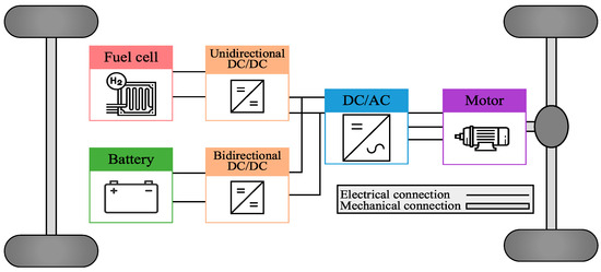
Figure 1.
Powertrain structure of fuel cell hybrid electric vehicle.

Table 1.
Main parameters of fuel cell hybrid electric vehicle.
2.1. Vehicle Dynamics Model
The powertrain must meet the driving requirements of the vehicle when the FCHEV is traveling on the road. According to the longitudinal dynamics of the FCHEV, the driving force can be expressed as:
where is the traction force of the vehicle, is the rolling resistance coefficient, is the mass of the FCHEV, is the angle of the road slope, is the frontal area, is the drag coefficient, is the vehicle rotational mass conversion coefficient, is the gravitational constant, and is the velocity. The total power balance equation is:
where is the power demand of the powertrain, is the fuel cell stack output power, is the battery output power, is the unidirectional DC/DC converter efficiency, and is the bidirectional DC/DC converter efficiency.
2.2. Fuel Cell Model
A proton exchange membrane fuel cell (PEMFC) was selected as the primary energy source due to its rapid startup capabilities, its high-power density, and the safety afforded by the solid electrolytes. The single fuel cell output voltage can be expressed as [29]:
where is the theoretical thermodynamic electric potential, is the activation loss, is the ohmic loss, and is the concentration loss. can be expressed as [30]:
where is the reference potential per unit of activity, is the Faraday constant, is the molar gas constant, and are, respectively, the varying partial pressures of hydrogen and oxygen, which can be obtained using the look-up table method. The fuel cell stack output power can be calculated as:
where is the number of single fuel cells, and is the single fuel cell current.
The fuel cell system net output power depends on the air compressor power loss and on the power losses of other components . The fuel cell system net output power can be expressed as:
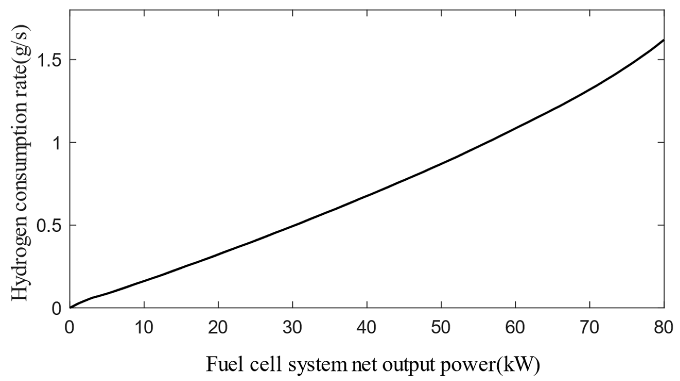
The fuel cell hydrogen consumption rate can be calculated as:
where is the hydrogen molar mass. The characteristic curve of the hydrogen consumption rate under the variation of the net output power of the fuel cell system is shown in Figure 2.
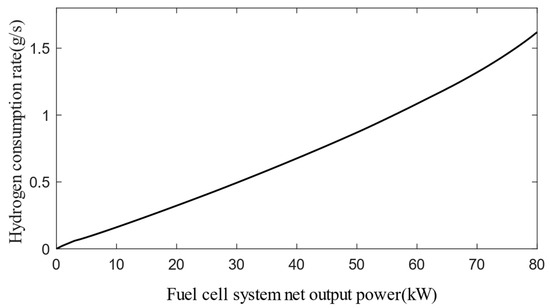
Figure 2.
Hydrogen consumption rate change characteristic curve.
The fuel cell system efficiency can be expressed as:
where LHV is the hydrogen low heating value, which has a value of 120,000 kJ/kg.
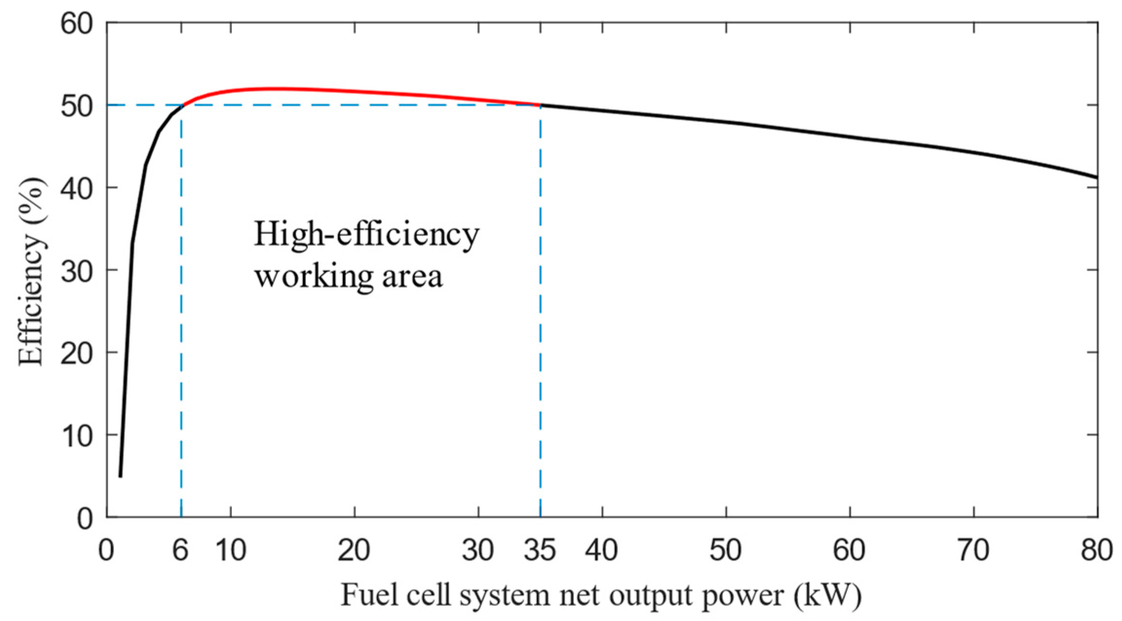
Figure 3 shows the relationship between the efficiency and the net output power when the fuel cell system is running. In order to improve the economy of the FCHEV, the fuel cell system should work more in the high-efficiency zone during the driving process. The part of the fuel cell system with an operating efficiency higher than 50% is defined as the high-efficiency operating area of the system, which is the operating area corresponding to a net output power of 8 to 36 kW in Figure 3.
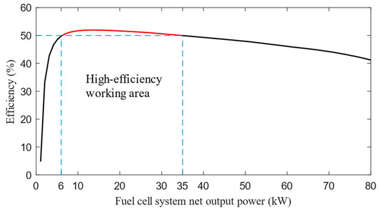
Figure 3.
Fuel cell system net power–efficiency curve.
Since the degradation problem was considered, it was important to construct a fuel cell degradation model. As a direct reflection of the fuel cell performance, the fuel cell stack voltage can sensitively respond to internal chemical changes and physical damage. Thus, the fuel cell stack voltage was chosen to characterize the fuel cell performance degradation. The voltage degradation of a single fuel cell can be expressed as:
where is the voltage degradation loss. Based on the degradation rates of the fuel cell performance tested by Pei et al. [31] under four different conditions–namely, start-stop, idling, a frequent variable load, and a high load–the voltage degradation rates of the fuel cell used in this study are summarized in Table 2.
Table 2.
Voltage degradation rates of fuel cell under different operating conditions.
According to the voltage degradation data of the fuel cell under different operating conditions in Table 2, the voltage degradation under each operating condition was calculated, and then the total voltage degradation of the fuel cell was obtained at the current moment t. The degradation voltage can be calculated as:
where is the start-stop condition voltage degradation, is the idling condition voltage degradation, is the frequent-variable-load condition voltage degradation, and is the high-load condition voltage degradation. , , , and are established based on the voltage degradation rates for the four operating conditions in Table 2, as follows:
The voltage degradation can be expressed as:
where is the fuel cell on/off status at the current moment t.
The voltage degradation can be calculated as:
where is the fuel cell power under the idling condition and is the idling operating time.
The voltage degradation can be defined by:
where is the fuel cell rated power.
The voltage degradation can be obtained by:
where is the high-load operating time.
2.3. Battery Model
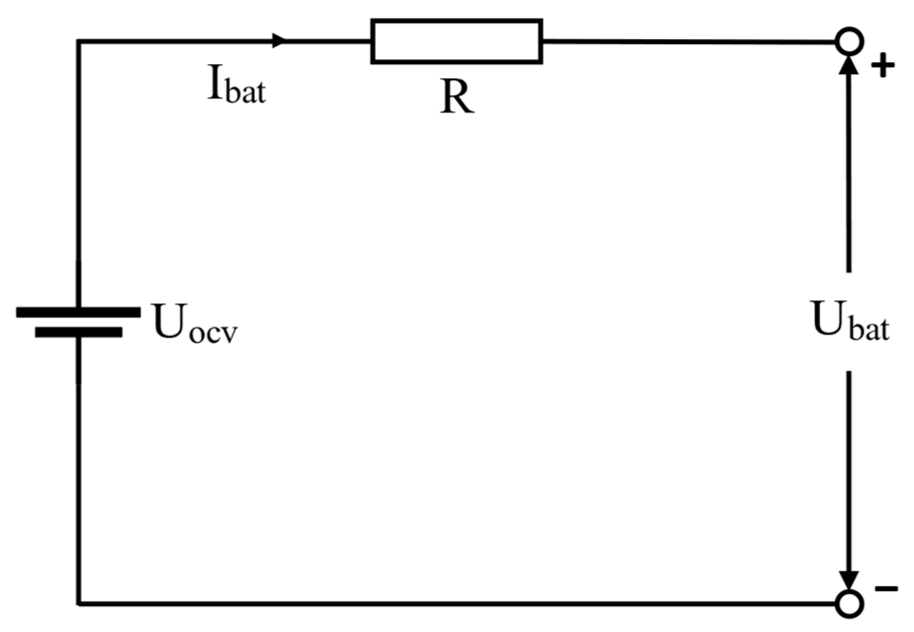
A lithium-ion battery with a high energy density and a high charge/discharge rate (C-rate) was selected as the battery, and the classical Rint internal resistance model was used to build the battery model. The equivalent circuit diagram is shown in Figure 4. According to the battery equivalent circuit diagram, the battery output power can be derived as:
where is the open-circuit voltage, is the internal resistance, and is the current.

Figure 4.
Battery equivalent circuit diagram.
The SOC was estimated by using the ampere–time integration method, and its expression is:
where is the initial state of charge, and is the nominal battery capacity.
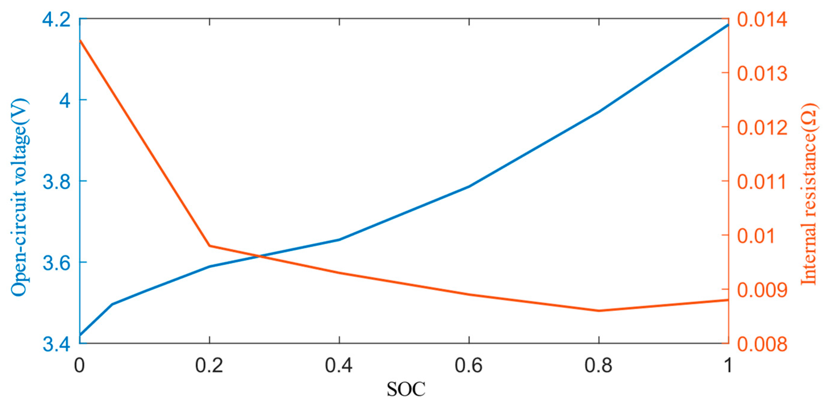
Based on Equations (15)–(17), the variations of the open-circuit voltage and internal resistance with the SOC are shown in Figure 5. As shown in Figure 5, as the SOC increases, the internal resistance of the battery will decrease gradually due to the increasing chemical reaction. However, when the SOC exceeds a certain value, the chemical reaction of the battery will become slower, and the internal resistance should hence rise again towards SOC = 1.
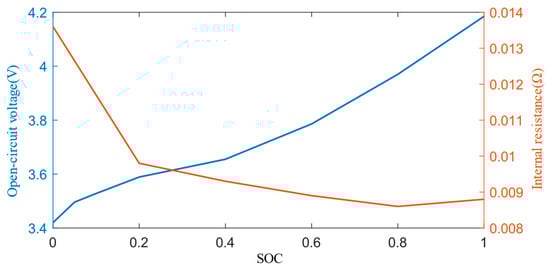
Figure 5.
Relationship between open-circuit voltage, internal resistance, and SOC.
The battery efficiency can be calculated as:
where is the discharged efficiency and is the charged efficiency. To facilitate the calculation of the hydrogen consumption of the FCHEV during driving, the hydrogen consumption rate of the battery can be expressed as:
Since the problem of battery performance degradation was considered, it was important to construct a battery performance degradation model. In the current semi-empirical modeling of battery performance degradation, researchers usually choose three key parameters—the internal resistance, the output power, and the capacity—as the characterization indices of battery performance. Due to the relative complexity of the degradation process of the battery power and of the internal resistance, it is difficult to build an accurate model for them. Therefore, the battery capacity was chosen to effectively evaluate and predict the battery performance degradation.
The generalized capacitance degradation model proposed by Li et al. [32] is as follows:
where is the battery capacity loss, is the pre-exponential factor, is the activation energy, is the temperature in Celsius, is the Ah-throughput, and is the power law factor which can be obtained from the capacity loss data. To further increase the accuracy of the power battery performance degradation model in the application of the EMS, Ye et al. [33] carried out a detailed parameter identification of the unknown parameters of the battery capacity degradation model. Based on this process, these identified parameters were applied to the generalized capacitance degradation model in this study to construct a more accurate battery performance degradation model based on capacity degradation, and the specific model is:
where and are the SOC-related coefficients that can be obtained by battery aging experiment and is the charge/discharge rate.
According to Equation (21), the degradation model of the battery includes the effect of the SOC, the temperature, and the charge/discharge rate on battery capacity decay.
2.4. Driving Motor Model
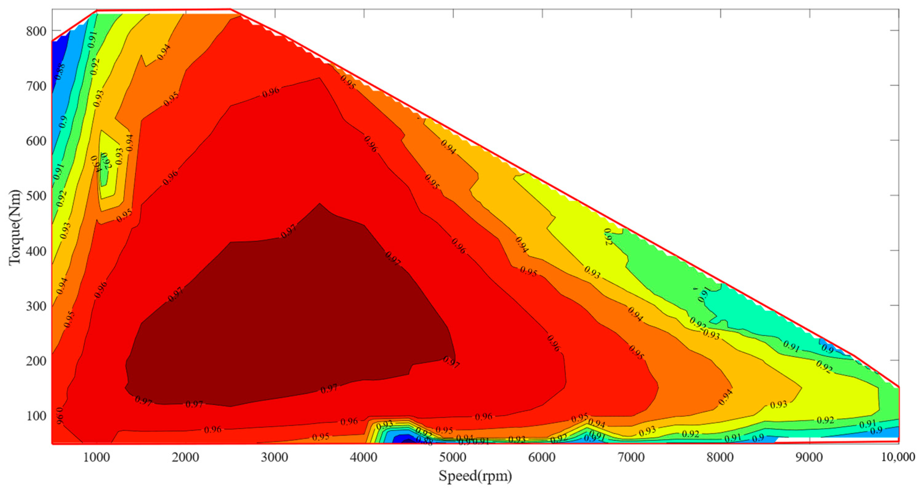
The drive motor is used as a mechanical power source for the FCHEV to propel the vehicle or for regenerative braking energy recovery. The motor model takes the motor torque and the motor speed as the inputs and the motor power for the output. The motor power can be calculated as:
where is the motor efficiency. The efficiency map of the drive motor is shown in Figure 6.
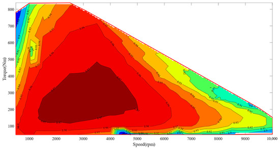
Figure 6.
Map of motor efficiency.
3. Energy Management Strategy of FCHEV
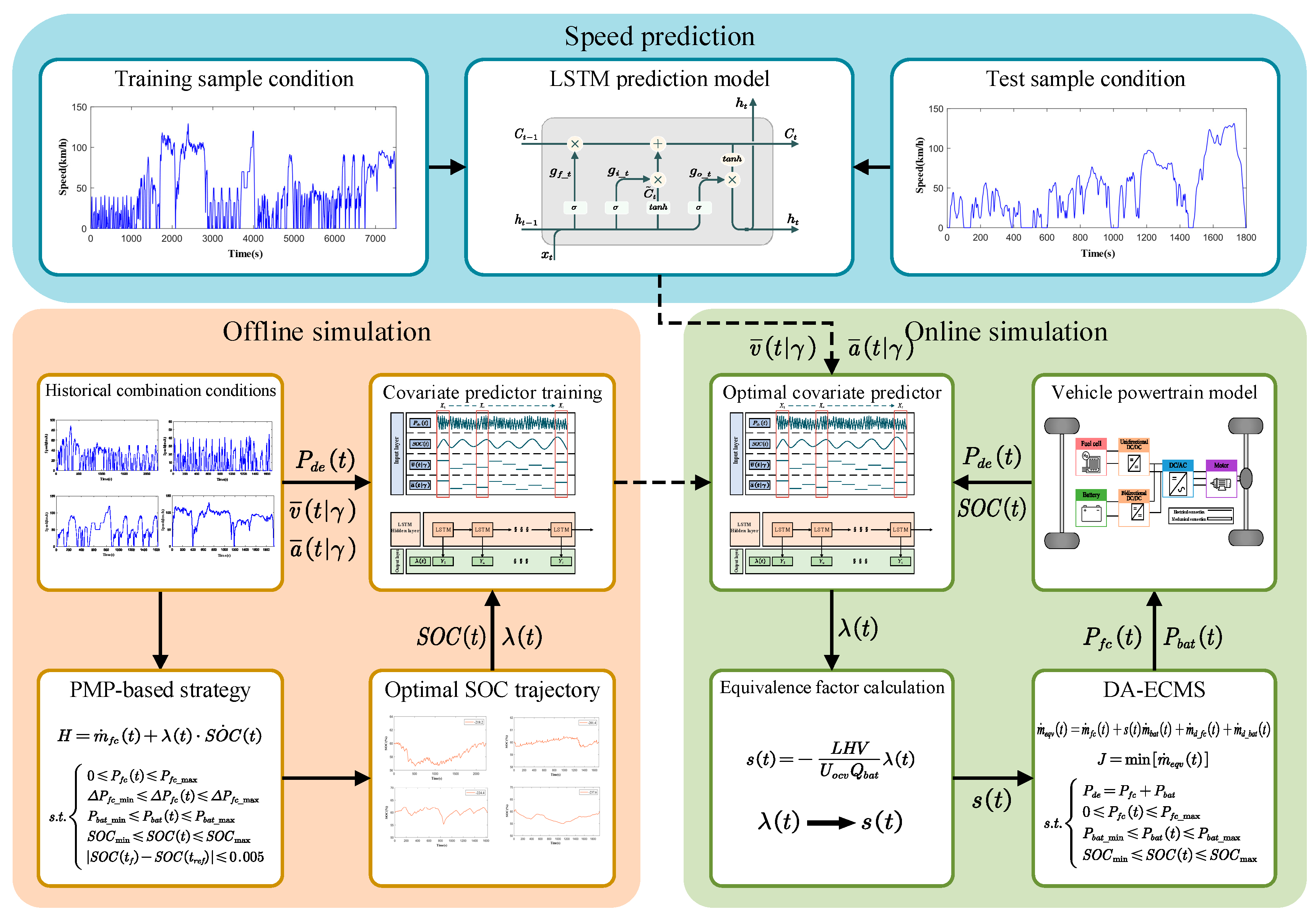
The DA-ECMS is constructed with three main parts, as discussed in this section: the speed prediction part, the offline part, and the online part. The overall framework of the strategy is shown in Figure 7. The speed prediction part is based on historical speed data and the speed prediction model is trained by an LSTM neural network. In the offline part, a database of the Hamiltonian function optimal covariates under different operating conditions is established, and the covariates in the database are used for the training of the optimal covariate predictor based on an LSTM neural network. In the online part, based on the equation relating the ECMS equivalent factor and the covariate, the optimal equivalent factor is predicted in real time, and the A-ECMS based on the optimal covariate predictor is constructed. Then, the performance degradation of the fuel cell and the battery is incorporated into the optimization objective of the A-ECMS, and the DA-ECMS is constructed.
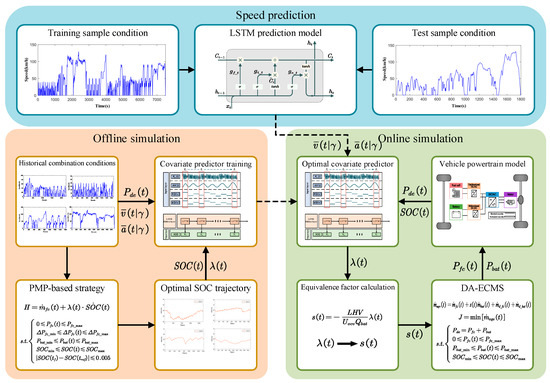
Figure 7.
Overall framework of energy management strategy.
3.1. Speed Prediction
An LSTM neural network is used to predict the future speed, which provides the speed data for the subsequent adaptive adjustment of the equivalence factor. To ensure that the proposed speed prediction model has a high prediction accuracy and effectiveness in a wide range of driving scenarios, eight combinations of driving conditions that cover most of the driving scenarios in daily life were used as the training sample database for the prediction model. The combined operating conditions are shown in Figure 7.
The acceleration and historical speed data were selected as the input of the LSTM neural network speed prediction model, and a multi-step prediction of the future speed was obtained by recursive methods. The specific steps of the model training and prediction were as follows:
- (1)
- Various driving conditions were combined to build a database of historical speed samples. The historical N s speed samples were selected in a sliding window and the acceleration corresponding to the vehicle speed at the current moment was introduced as a characteristic parameter to build the input and the output vectors :
- (2)
- The size of the training sample data set was S. The sliding step was set to 1 s, and the model selected the first N s historical speed data of the training sample database to train based on the sliding step. The model training sample input matrix and output matrix were then obtained:
- (3)
- After the training of the LSTM speed prediction model was complete, the first N s historical speed data in the test sample database were selected as the sliding window, and the historical speed data were input into the trained model according to the input matrix of the test sample to predict the speed 1 s in the future. At this time, the sliding window was shifted to the right in accordance with the step length, and the 1 s speed data obtained from the prediction was added to the right side of the sliding window to form a new input, which was then input into the model to predict the speed 2 s in the future. The above operation was repeated to realize the multi-step prediction of the future speed.
3.2. Optimal Covariate Predictor Based on Long Short-Term Memory Neural Network
In order to realize the real-time adjustment of the covariate, an optimal covariate predictor was proposed. Specifically, the predictor was based on an LSTM neural network for optimal covariate prediction, and the training samples of the LSTM neural network were the optimal covariate database built based on Pontryagin’s minimum principle (PMP).
3.2.1. Optimal Covariate Database Based on PMP
PMP was used to predict the covariate, and the optimization objective was minimum hydrogen consumption under known operating conditions within the time boundary. The output power of the fuel cell stack was chosen as the control variable, and the SOC was chosen as the state variable. The objective function is expressed as:
where is the fuel cell instantaneous hydrogen consumption, is the start point, and is the end point. is the terminal SOC cost function, which can be expressed as:
where is the SOC lower limit, is the SOC upper limit, and 10,000 is a very large constant value, which allows the optimization to remain within constraints.
The energy source output power should satisfy the following power balance equation:
where is the power demand. The state equation is defined as:
where is the battery open-circuit voltage corresponding to the SOC at the current moment t and is the instantaneous SOC change rate. The control variable and the state variable in the optimization problem are subject to the following constraints:
where the fuel cell stack maximum output power was set to 82 kW, the lower limit and upper limit of the permissible fuel cell stack power change were −10.4 and 5.4 kW, respectively, the lower limit and upper limit of the battery power were −80 and 80 kW, respectively, the lower limit and upper limit of the SOC were 0.2 and 0.8, respectively, is the SOC at the end of the calculation, and is the reference state variable.
The Hamiltonian function is defined as follows:
where is the covariate. The optimal control variable can be expressed by the following equation:
where is the optimal state variable, and is the optimal covariate. must satisfy the following conditions:
- (1)
- must be obtained such that the Hamiltonian function achieves the minimum of all values within the time boundaries, as follows:
- (2)
- The optimal state variable equation is obtained by partial differentiation of the covariate in the Hamiltonian function, as follows:
The optimal covariate trajectory equation is obtained by partial differentiation of the state variable in the Hamiltonian function, as follows:
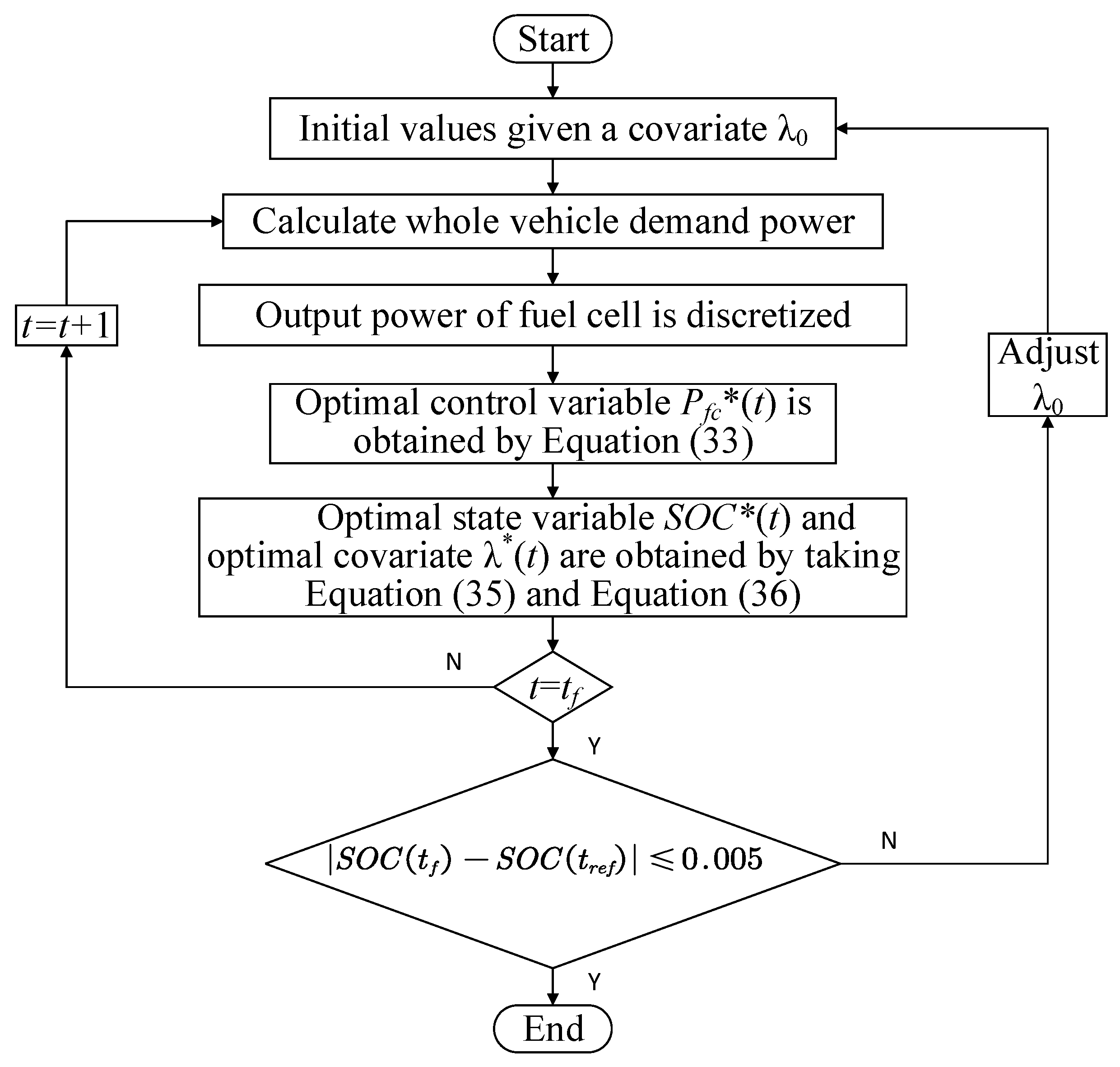
When solving the optimization problem using PMP, the initial value of the covariate is usually unknown, and the determination of the initial value of the covariate needs to be carried out by using corresponding search methods. The target method was chosen to solve for the initial covariate, and the reference state variable was set to 0.6. The steps were as follows:
First, a guess of the initial covariate was provided. Second, the FCHEV power demand was calculated from the known operating conditions. Then, the fuel cell stack output power was discretized within the constraint interval, and the optimal control variable was calculated by Equation (34). Finally, the optimal state variable and optimal covariate were derived by substituting them into Equations (36) and (37). After the calculation, was compared with . If the difference was within the set threshold, then the cycle was not repeated, and the current covariate was output as the optimal covariate; otherwise, the current covariate was adjusted and the above steps were repeated until the optimal covariate was obtained that met the threshold value, as shown in Figure 8.
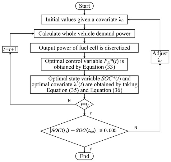
Figure 8.
Pontryagin’s minimum principle solution steps.
In order to make the covariate predictor closer to the optimal covariate predictor, four driving conditions–namely urban smooth, urban congested, suburban, and highway conditions–were selected so that the optimal database could cover the optimal SOC trajectories and the optimal covariates under various driving conditions as much as possible. The initial SOC was set to 0.6, and the PMP-based strategy was implemented offline under the four combined driving conditions to obtain the optimal covariate and the corresponding optimal SOC trajectory under each condition, as shown in Figure 7. At this point, the historical speed data under the four different operating conditions were input into the model, and the corresponding power demand data were calculated and integrated with the optimal SOC trajectory and optimal covariate to construct the optimal covariate database.
3.2.2. Optimal Covariate Predictor
In practice, due to the unpredictability of future driving conditions, the optimal covariate in the PMP has a great deal of uncertainty, so it is difficult to plan it in advance. In order to improve the adaptability to future driving conditions, it is necessary to establish the relationship between the driving conditions, the real-time vehicle states, and the optimal covariate. LSTM neural networks are good at solving complex nonlinear problems, and they are especially suitable for modeling tasks with high complexity and fuzzy inference rules. Therefore, the optimal database obtained from the PMP solution was substituted into the LSTM neural network model for training and learning to determine the optimal covariate predictor.
Considering the tradeoff between the prediction speed and the accuracy of LSTM, the optimal covariate predictor chose 5 s as the prediction time domain. The optimal covariate is related to the driving conditions and the current state of the powertrain, and these two factors need to be considered when estimating and predicting the coefficient. The current power demand and the SOC describe the real-time state of the powertrain system of the FCHEV, while the speed and acceleration in the next 5 s characterize the driving conditions. Therefore, the input parameters of the LSTM neural network model are the SOC of the powertrain, the vehicle power demand, the average speed in the next 5 s, and the average acceleration in the next 5 s. The output layer parameters of the model were set to the optimal covariate at the current time, as shown in Figure 7, in the offline section.
The optimal database constructed based on the PMP was used as the training sample data set of the LSTM prediction model, and the Worldwide Harmonized Light Vehicle Test Procedure (WLTP) and the China Light-Duty Vehicle Test Cycle (CLTC), which cover a variety of driving scenarios, such as urban, highway, and suburban areas, were chosen as the test sample data. By constantly adjusting the model hyperparameters during model training and testing, the error values between the predicted optimal covariate and the real optimal covariate were compared. The LSTM prediction model with the best training effect was used as the optimal covariate predictor for the subsequent real-time adjustment of the equivalence factor. The LSTM neural network prediction model hyperparameters were set as shown in Table 3.
Table 3.
Selected hyperparameters of optimal covariate predictor.
The sampling time of the historical sample had a significant effect on the prediction accuracy of the covariate. It was shown that the sampling time of the historical sample data was more reasonable in the range of 80 to 150 s [34]. Therefore, the sampling time of the historical sample data was set to 100 s. The covariates were categorized according to the four different driving conditions, as shown in Table 4. The prediction results of the covariate will be analyzed in Section 4.
Table 4.
Optimal covariate.
3.3. DA-ECMS
The ECMS converts the electrical energy consumption of the battery into an equivalent hydrogen consumption by setting an equivalence factor, which in turn calculates the total hydrogen consumption rate minimum at each moment. The instantaneous total hydrogen consumption rate of the FCHEV can be expressed as:
where is the fuel cell instantaneous hydrogen consumption rate and is the equivalence factor.
The optimization objective of the ECMS is to minimize the instantaneous total hydrogen consumption rate. Thus, the optimization objective function is defined as:
can also be expressed as a function of :
The relationship between the covariates and the equivalence factors can be derived as:
The speed prediction model and the optimal covariate predictor constructed in the previous section are combined with the ECMS to construct an A-ECMS. Compared to the fixed equivalence factor of the ECMS, the equivalence factor of the A-ECMS can vary with the change of the operating conditions.
The performance degradation of the fuel cell and the battery is incorporated into the optimization objective of the A-ECMS, in which case the total instantaneous hydrogen consumption rate considering performance degradation of the FCHEV can be expressed as:
where is the equivalent hydrogen consumption rate of the fuel cell performance degradation and is the equivalent hydrogen consumption rate of the battery performance degradation. The objective function of the DA-ECMS is defined as:
Compared to the A-ECMS, the DA-ECMS considers the performance degradation of the energy sources. The fuel cell stack was considered to have failed when its performance degradation reached 10%. The ideal output voltage of the fuel cell stack is 300 V in this study. can be expressed as:
where is the fuel cell stack performance degradation rate, is the fuel cell stack price, and is the hydrogen price.
The battery is considered to have failed when its performance degradation reaches 20%. can be expressed as:
where is the battery price. In this optimization problem, the fuel cell stack output power , the battery output power , and SOC should satisfy the following constraints:
4. Simulation Results and Discussion
The proposed optimal covariate predictor and DA-ECMS were validated through simulations performed in MATLAB/Simulink R2023a on a PC with an Intel (R) Core (TM) i5-9300H @ 2.40 GHz and 16 RAM (Intel, Santa Clara, CA, USA).
4.1. Result of Optimal Covariate Prediction
The prediction results of the optimal covariate under the WLTP and the CLTC are shown in Figure 9 and Figure 10, respectively. The vertical coordinates in these figures represent the optimal covariate value numbers for each operating condition, as shown in Table 4. The prediction accuracy of the predictor model was 91.44% under the WLTP and 88.17% under the CLTC. The predictor maintained a high prediction accuracy under both test conditions, which indicated that the optimal covariate predictor established had good adaptability to the operating conditions and a good prediction effect under the different operating conditions.
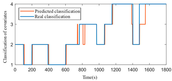
Figure 9.
Prediction of optimal covariate under Worldwide Harmonized Light Vehicle Test Procedure (WLTP).
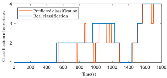
Figure 10.
Prediction of optimal covariate under China Light-Duty Vehicle Test Cycle (CLTC).
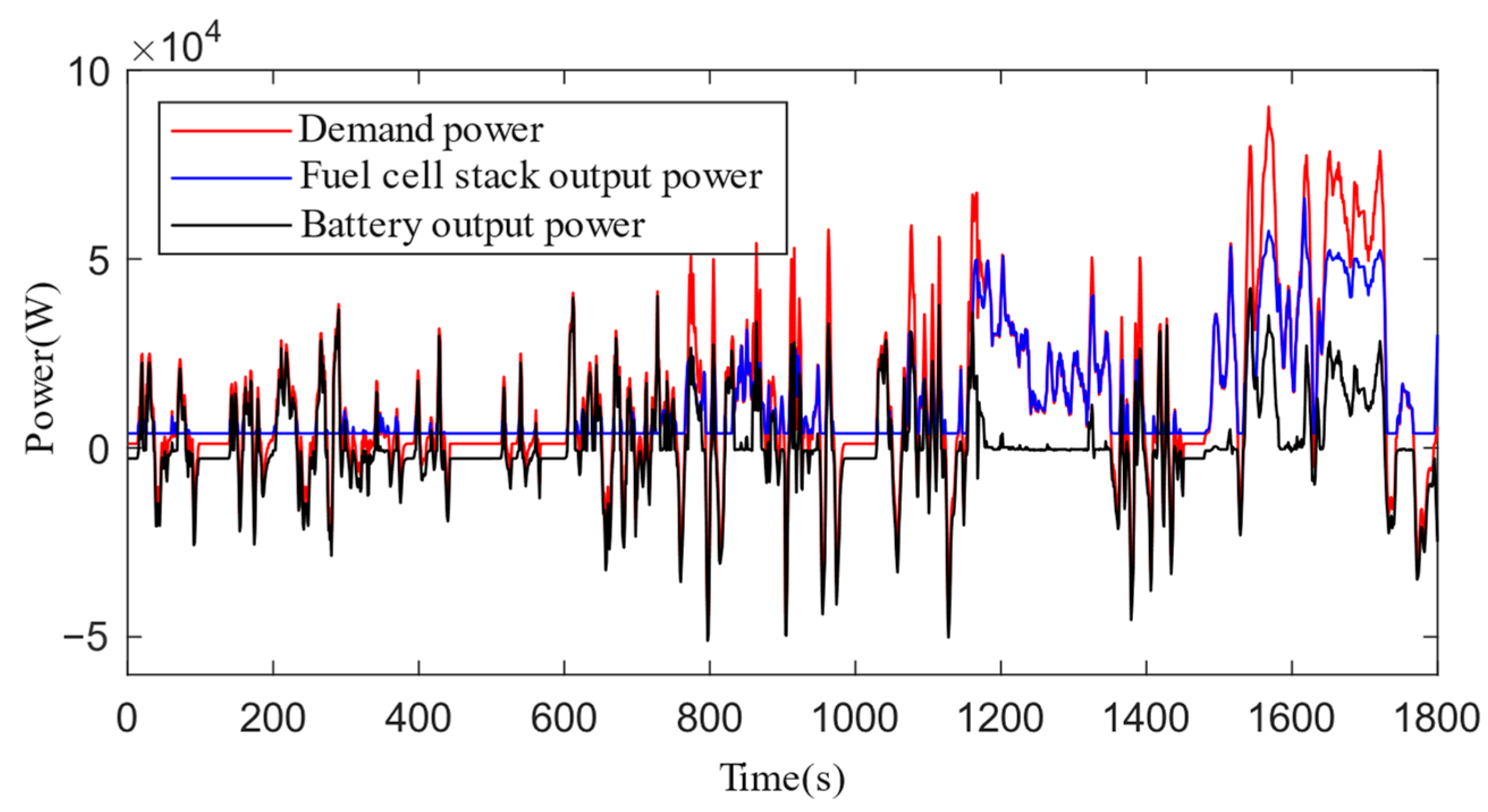
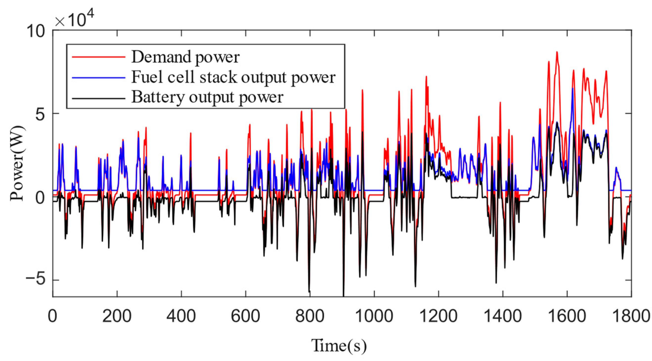
The WLTP was selected to validate the A-ECMS based on covariate prediction using the ECMS as a reference. The results of the hybrid energy source power distribution under the A-ECMS based on covariate prediction and the ECMS are shown in Figure 11 and Figure 12, respectively. Compared with the power distribution under the ECMS, the fuel cell stack output power in the A-ECMS was more continuous, with fewer fluctuations and peaks, which was conducive to the improvement of the fuel cell durability.
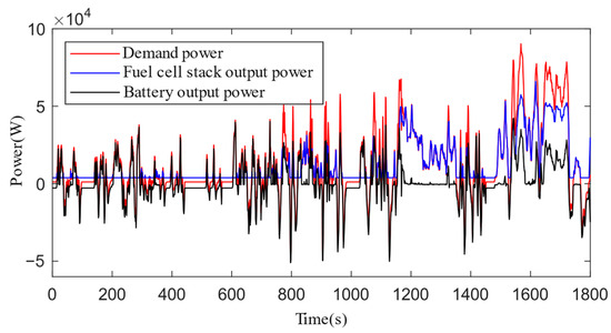
Figure 11.
Hybrid energy source power allocation result under adaptive equivalent consumption minimization strategy (A-ECMS).
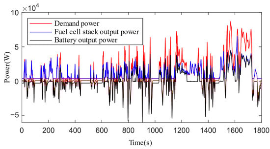
Figure 12.
Hybrid energy source power allocation result under equivalent consumption minimization strategy (ECMS).
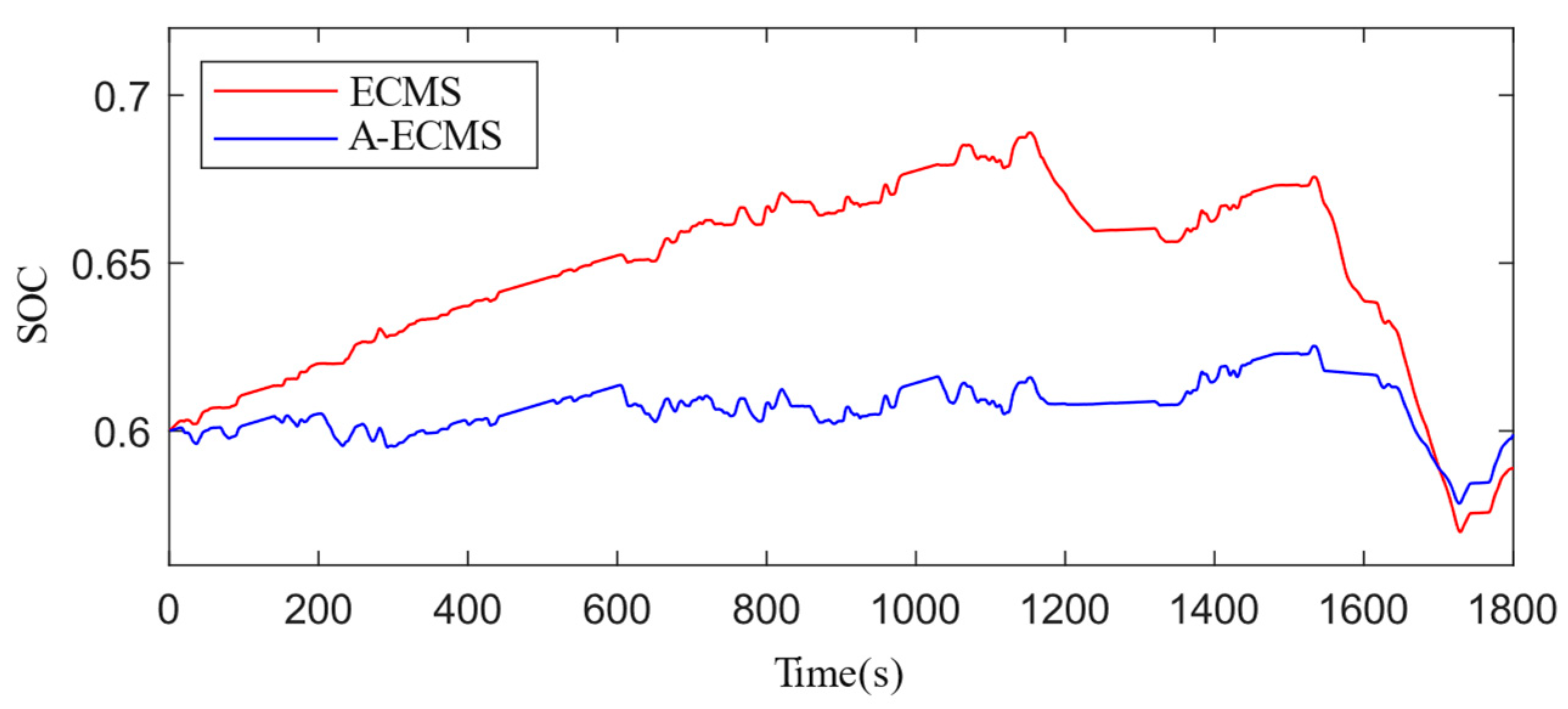
The trajectory of the SOC is shown in Figure 13. The SOC under the ECMS was more volatile than under the A-ECMS, and the A-ECMS could effectively control the SOC fluctuation range due to the real-time adjustment of its equivalence factor. In addition, the A-ECMS could stably adjust the SOC back to around 0.6 at the end of the simulation to maintain stable battery power.
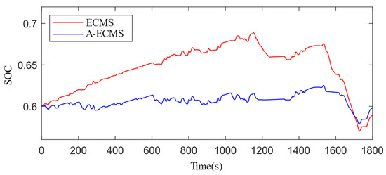
Figure 13.
State of charge (SOC) trajectories under ECMS and A-ECMS.
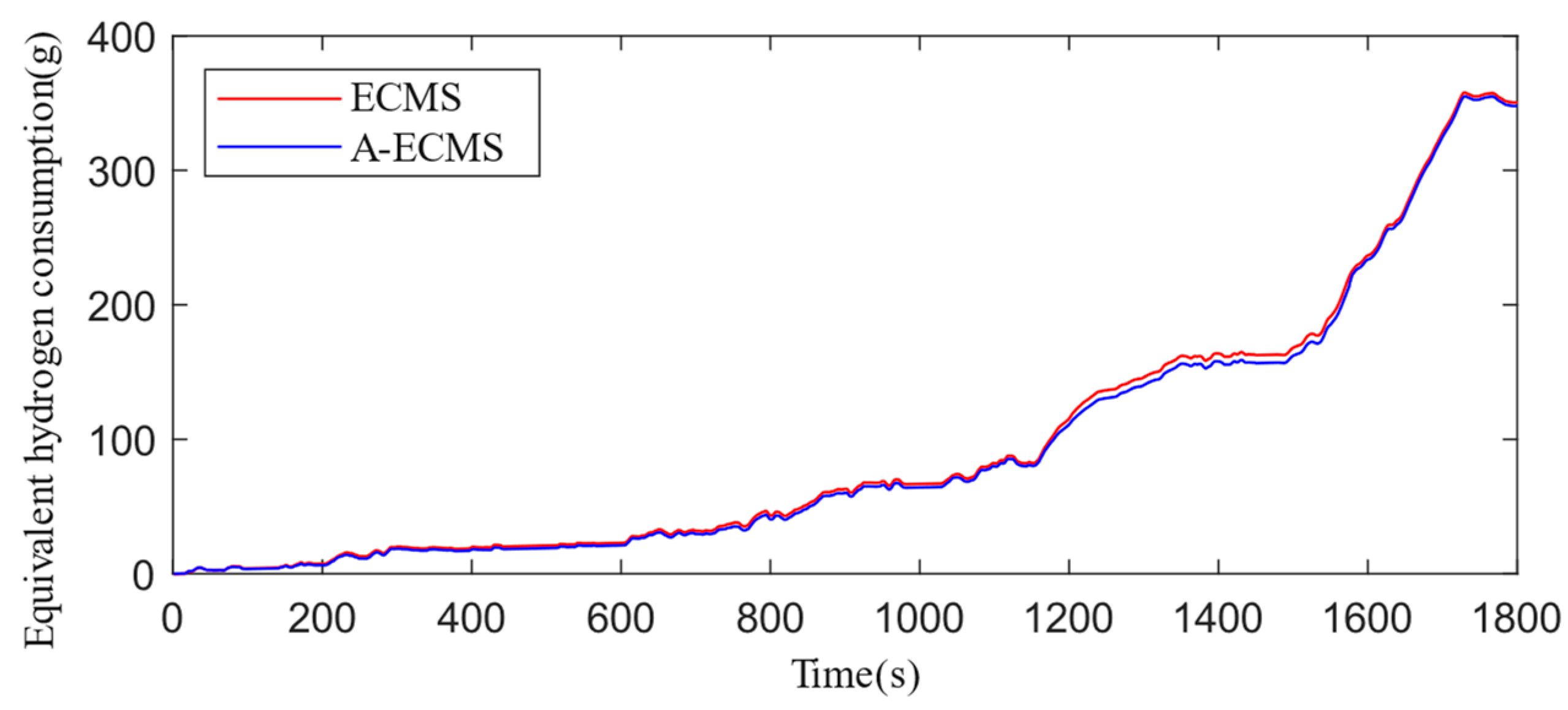
The trajectory of the equivalent hydrogen consumption is shown in Figure 14. The final value of equivalent hydrogen consumption was 355.9 g under the ECMS and 350.6 g under the A-ECMS, and the value for the A-ECMS was thus 1.5% lower. The value was smaller because certain prediction errors could easily occur in the process of speed prediction and determination of the equivalence factor, and the A-ECMS needed to consider the maintenance of the battery power while optimizing the overall vehicle economy to reduce the fluctuations of the battery SOC. However, the equivalence factor selected under the ECMS was the best equivalence factor under the test conditions, so the optimization effect of the A-ECMS was not significant enough under this condition.
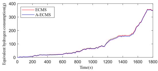
Figure 14.
Equivalent hydrogen consumption curves under ECMS and A-ECMS.
4.2. Comparative Validation of DA-ECMS
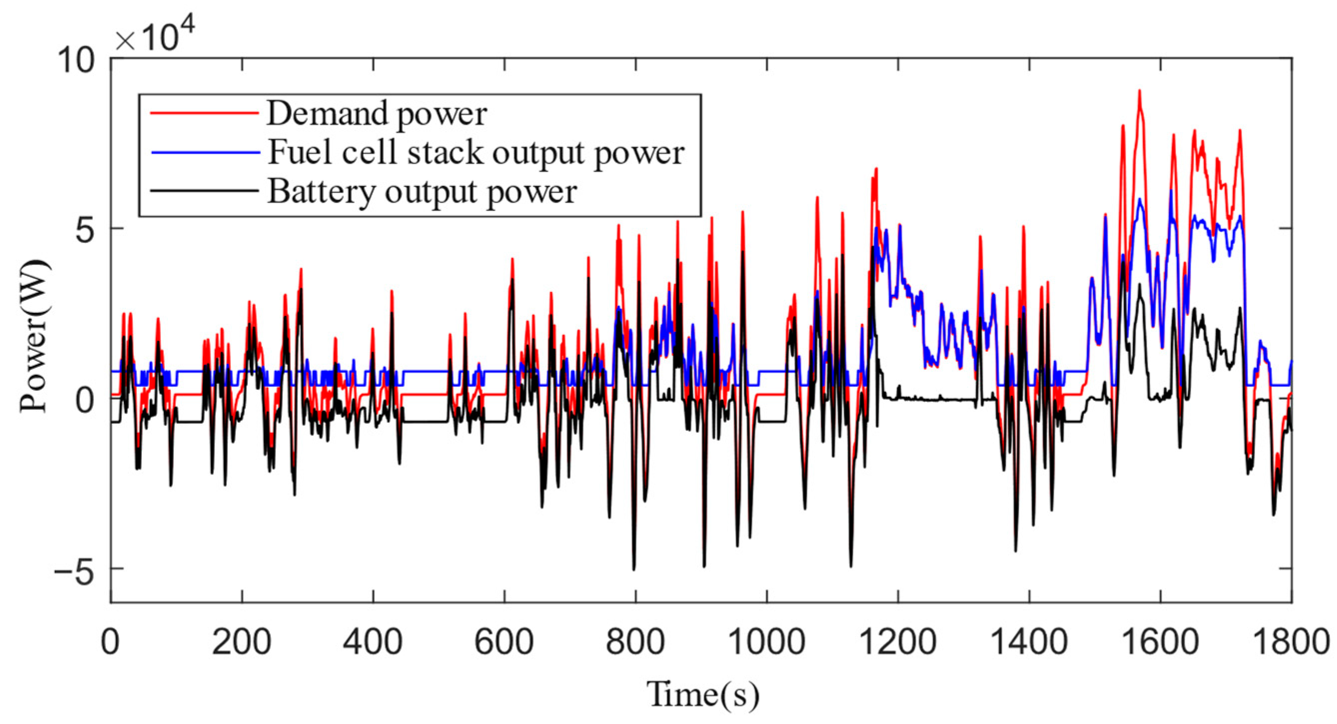
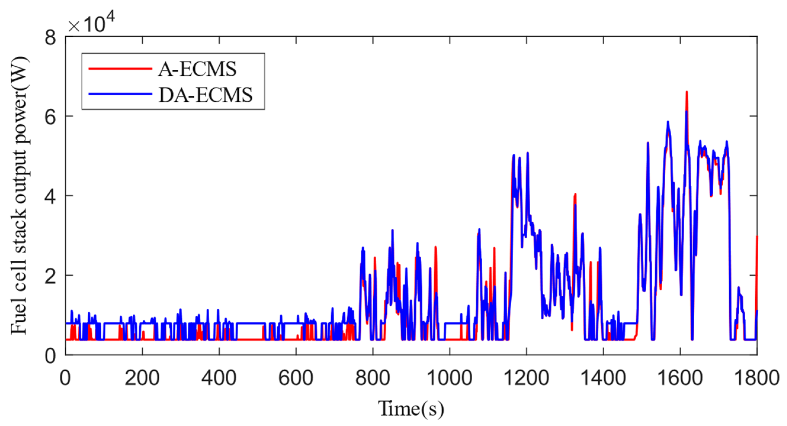
The DA-ECMS was verified under the WLTP. The result of the hybrid energy source power allocation in this strategy is shown in Figure 15. The trajectory of the fuel cell stack output power is shown and compared with the corresponding changes under the A-ECMS in Figure 16. The FCHEV power demand was low in the first 780 s of the test conditions. At this time, the battery was the main source of the power output, while the fuel cell stack was running in a lower-power state, basically in the idling state. In order to reduce the fuel cell degradation in the idling operation, the DA-ECMS increased the fuel cell stack output power and stabilized it at 8.3 kW, while charging the battery at the same time. Compared with the results for the A-ECMS, the fuel cell stack output power fluctuations and peaks occurred less frequently in this strategy, which helped prevent fuel cell performance degradation due to frequent load changes. In the second half of the test conditions, the FCHEV power demand rose, and the fuel cell stack supplied the main power output. By precisely adjusting the power distribution, the DA-ECMS effectively avoided the operation of the fuel cell under high-power conditions, which prolonged the fuel cell lifetime.

Figure 15.
Hybrid energy source power allocation result under adaptive equivalent consumption minimization strategy considering performance degradation (DA-ECMS).
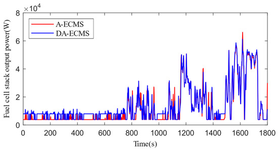
Figure 16.
Fuel cell stack output power change trajectory under A-ECMS and DA-ECMS.
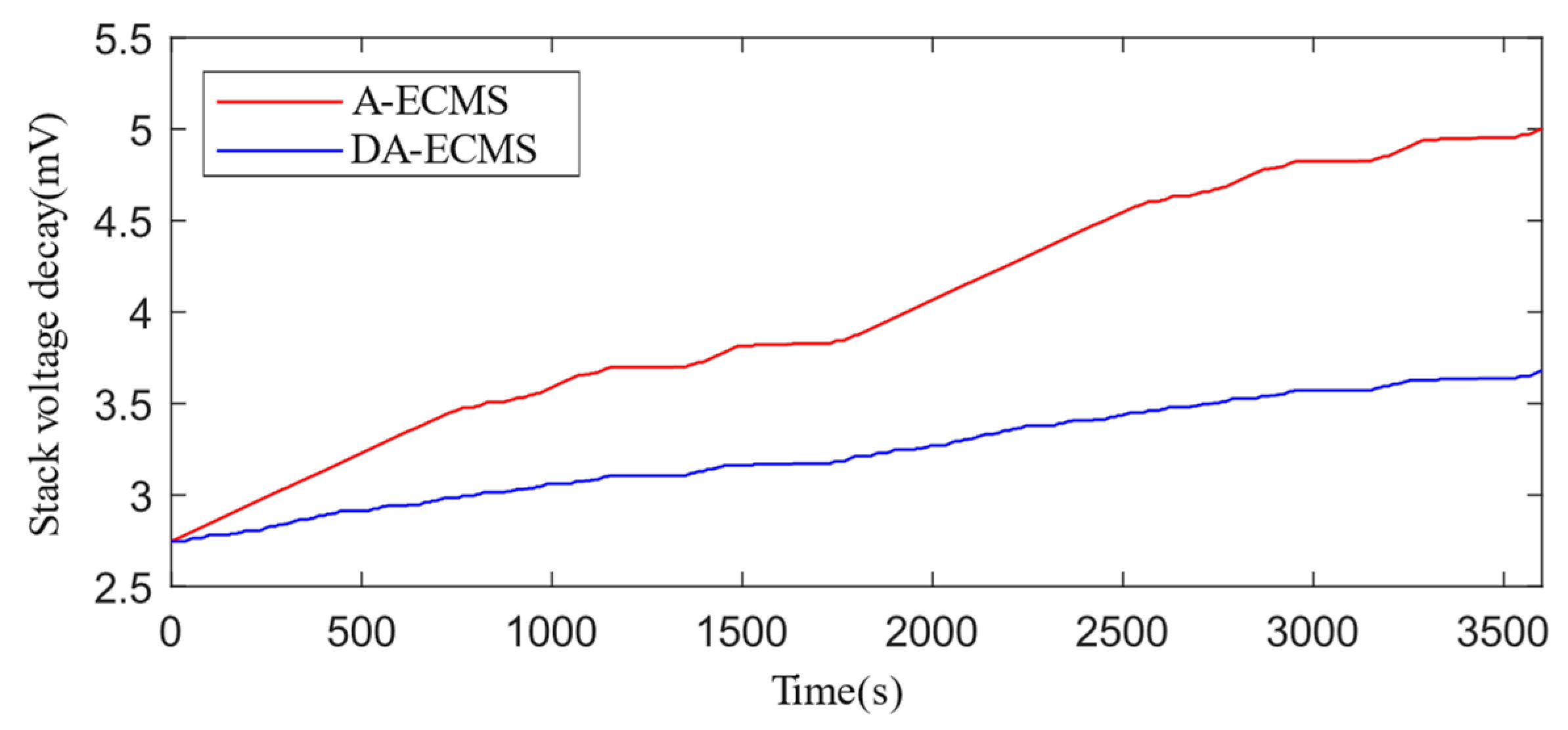
Since the WLTP test duration is 1800 s, two WLTP processes were selected to form a combined condition to simulate the voltage degradation of the fuel cell stack under different strategies for 1 h, and the test result is shown in Figure 17. The voltage degradation caused by the poor operating conditions of the fuel cell stack under the DA-ECMS was 3.679 mV, which was 1.322 mV lower than that of the A-ECMS. Only the voltage degradation of the starting part in the start-stop condition is shown in the figure. After adding the voltage degradation caused by the stopping part, the total voltage degradation was 6.425 mV, which was 17.1% lower than that of the A-ECMS and effectively slowed down the performance degradation of the fuel cell.

Figure 17.
Fuel cell stack voltage degradation under A-ECMS and DA-ECMS.
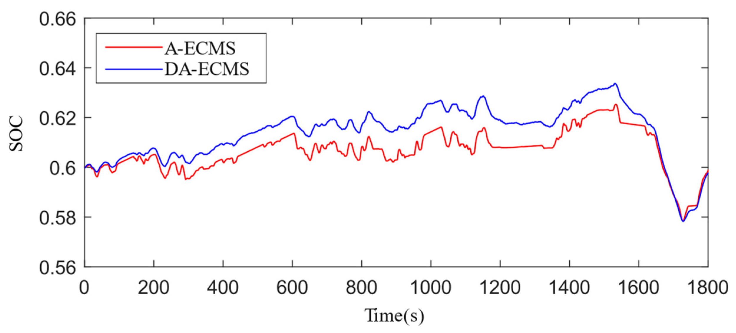
The SOC trajectory and the C-rate of the battery under the A-ECMS and the DA-ECMS are shown in Figure 18 and Figure 19, respectively. To avoid the prolonged inefficient operation of the fuel cell and frequent load changes, the DA-ECMS increased the fuel cell stack output power and used the extra power to charge the battery, resulting in an overall slightly higher SOC than that under the A-ECMS. Compared with the A-ECMS, the DA-ECMS had a smaller change in the C-rate of the battery, which effectively slowed the performance degradation of the battery.
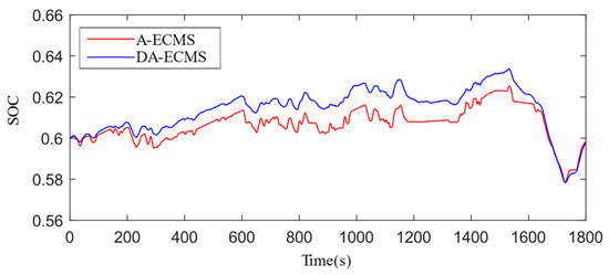
Figure 18.
SOC trajectory of battery.
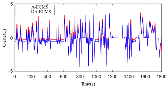
Figure 19.
C-rate of battery.
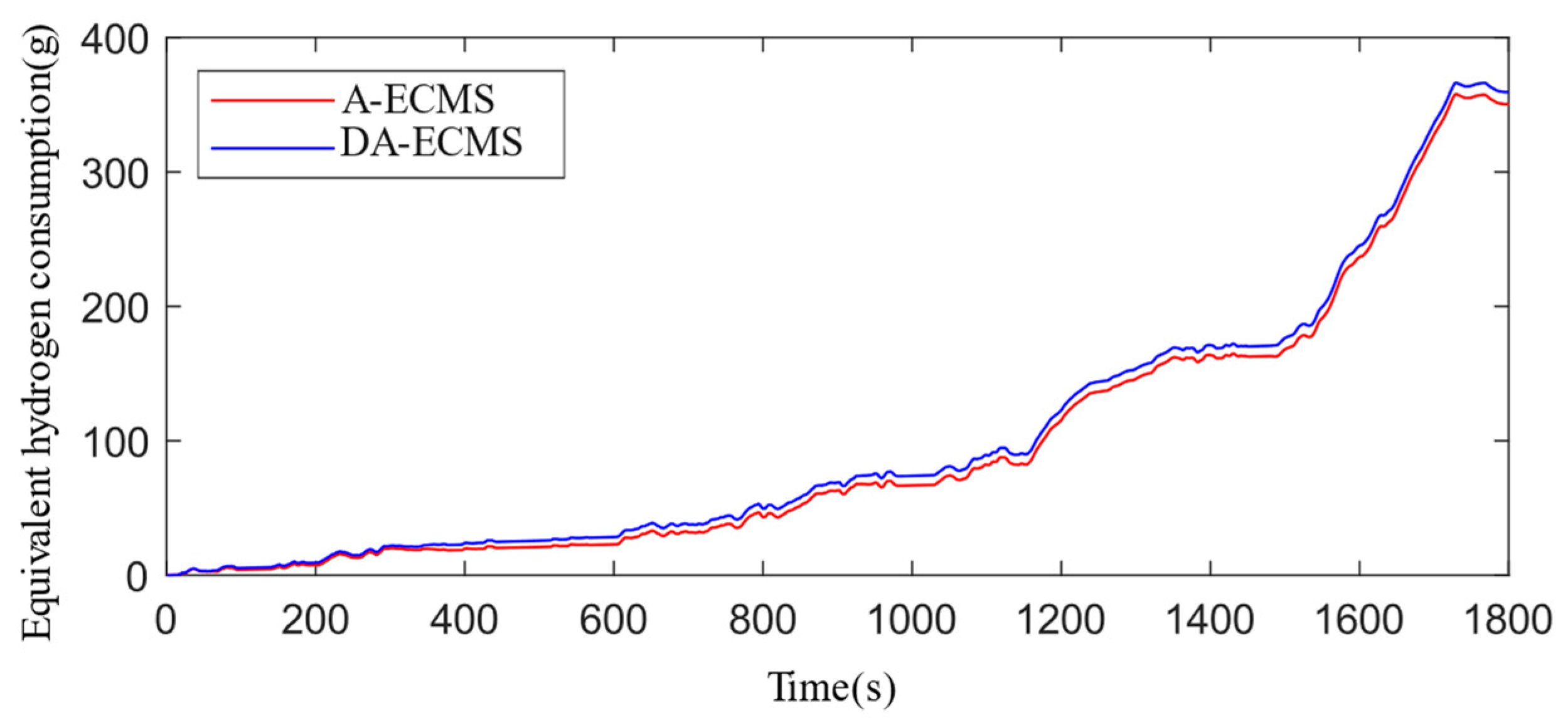
The A-ECMS and DA-ECMS equivalent hydrogen consumption curves are shown in Figure 20. The DA-ECMS not only pursued economy in power allocation but also considered the hybrid energy source’s long-term stability to ensure the power system’s continuous health and efficient operation. As a result, the final equivalent hydrogen consumption of the DA-ECMS reached 359.5 g, which was an increase of 2.5% compared with that of the A-ECMS.
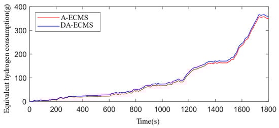
Figure 20.
Equivalent hydrogen consumption curves.
The A-ECMS and DA-ECMS were simulated under different operating conditions, and the validation results are shown in Table 5. From the analysis of the data in Table 5, it can be seen that, compared with the A-ECMS, the DA-ECMS effectively improved the performance degradation of the hybrid energy source while sacrificing a small amount of fuel economy. Therefore, in contrast with A-ECMS, the DA-ECMS could balance the FCHEV economy and energy source durability, and it had good adaptability to the operating conditions. Compared with the WLTP and the CLTC, there are more operational conditions of start-stop and variable load in NEDC, and the start-stop and variable load will aggravate the performance degradation of the energy source. Therefore, in order to improve the lifetime of the energy source, the hydrogen consumption increasement under the NEDC is the highest among the three operating conditions. Compared to A-ECMS, under the NEDC, the hydrogen consumption of DA-ECMS over 100 km increased by 9.1%.
Table 5.
The simulation results of the A-ECMS and DA-ECMS under different operating conditions.
5. Hardware-in-the-Loop Validation
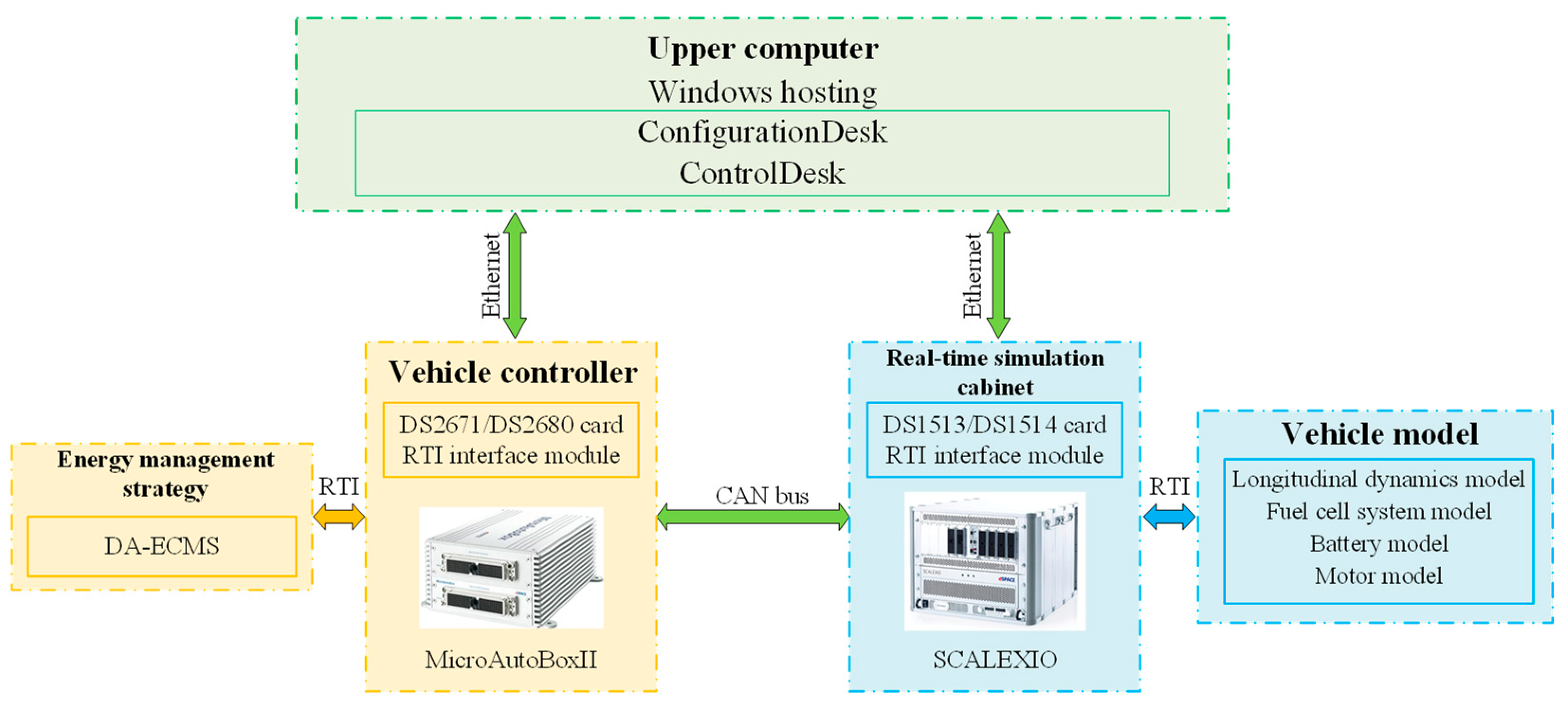
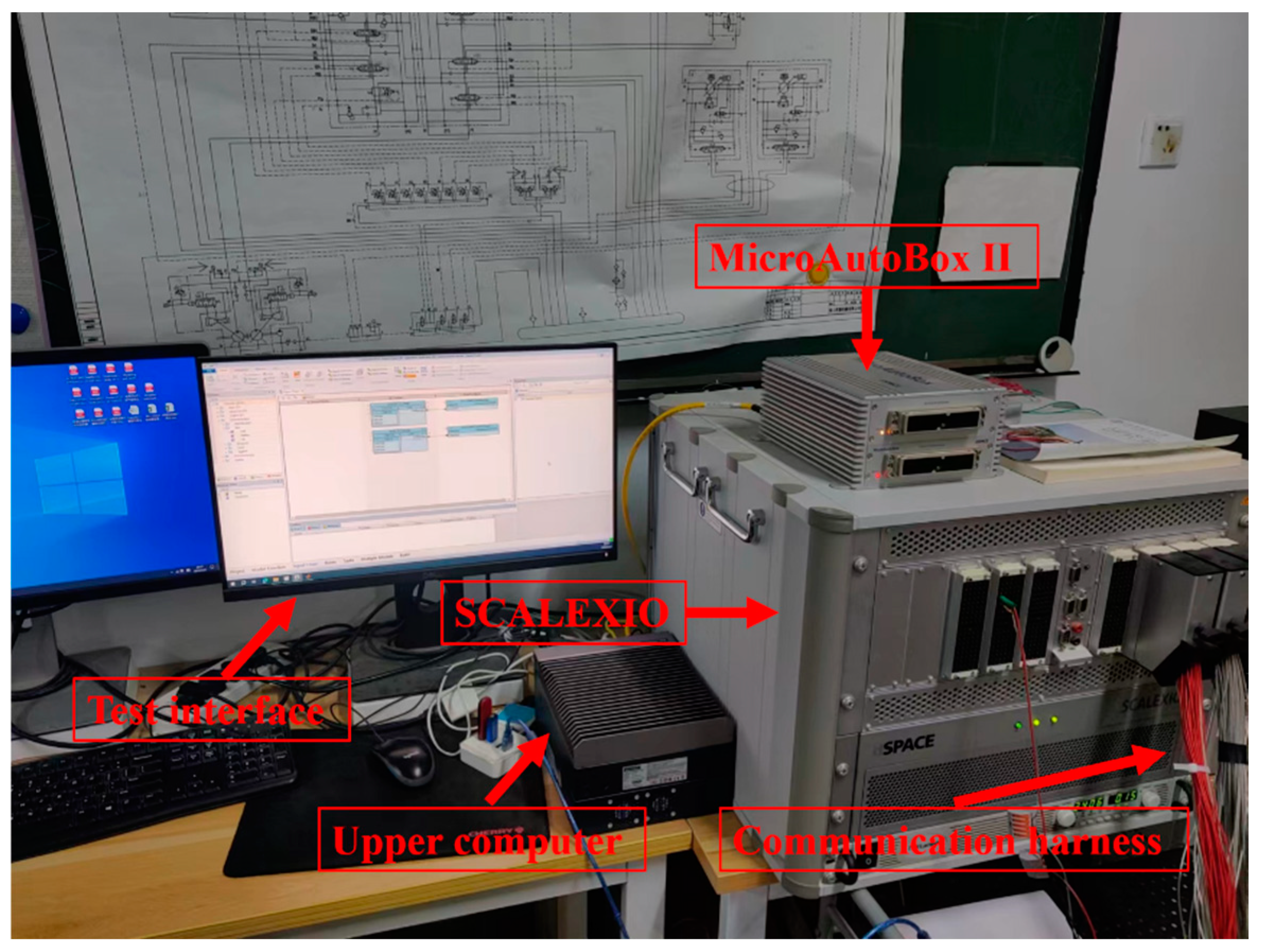
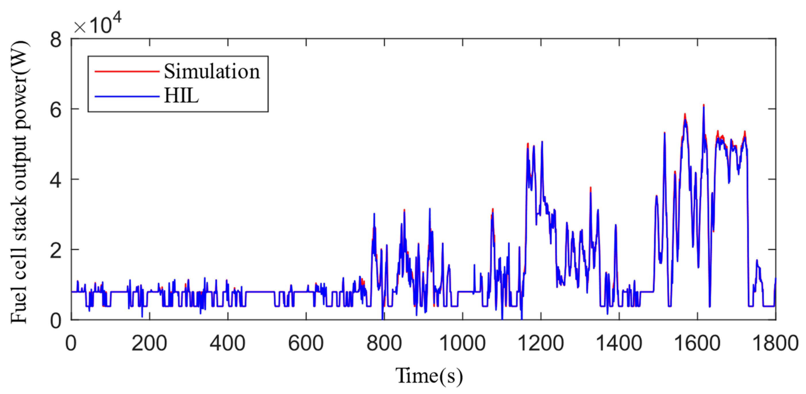
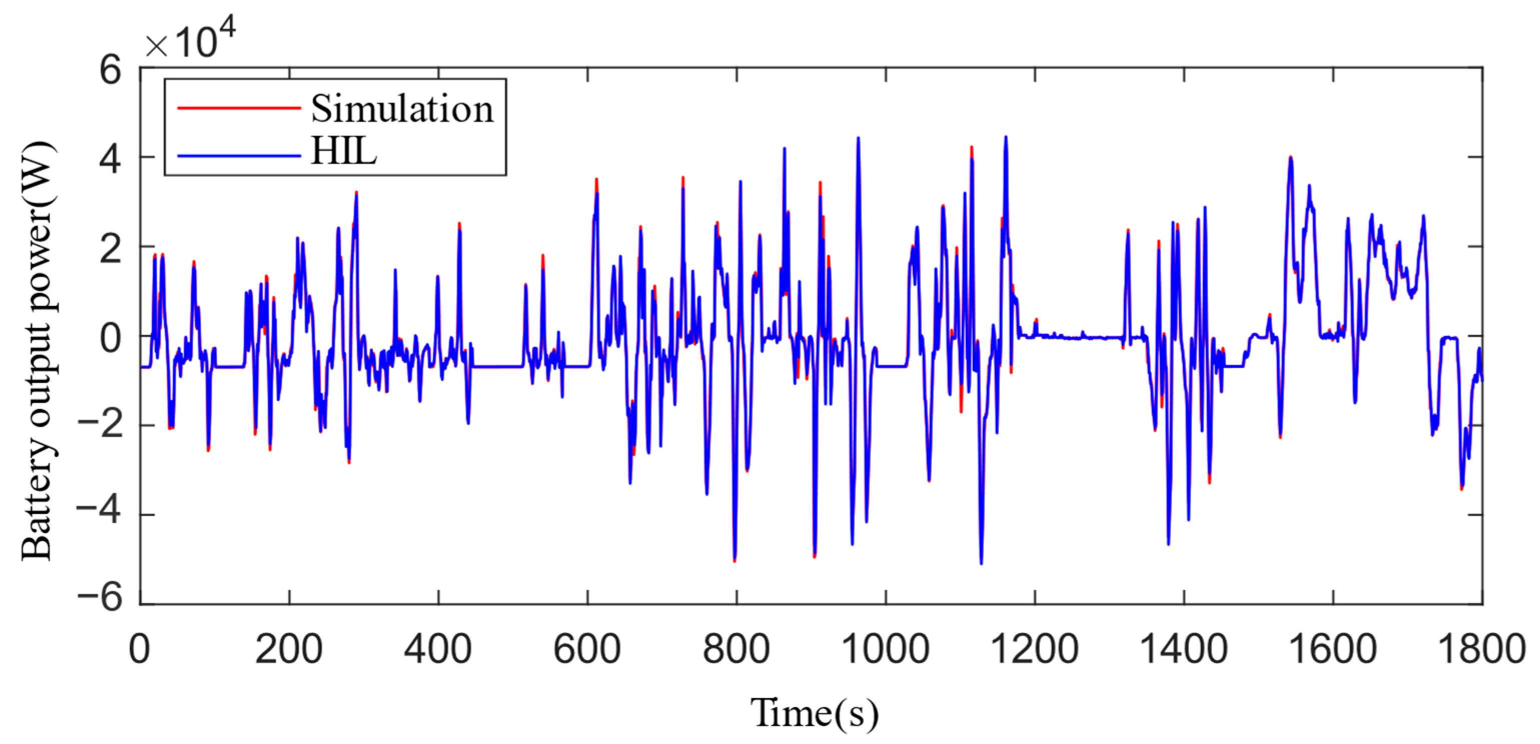
In order to demonstrate the optimization effect of the DA-ECMS in a real vehicle system, a hardware-in-the-loop (HIL) test was used to validate the optimization effect under the same WLTP conditions as in the above simulation validation. A dSPACE experimental bench was constructed to simulate the dynamic conditions and signal interactions in a real vehicle environment, which is provided by dSPACE GmbH from Paderborn, Germany. The overall frame diagram of the experimental bench and the diagram of the experimental bench are shown in Figure 21 and Figure 22, respectively. The test results of the fuel cell stack and battery output power from the simulation and HIL tests are shown in Figure 23 and Figure 24, respectively. The overall trends of the fuel cell stack and battery output power were basically the same, and the errors and delays mostly appeared at their power peaks.
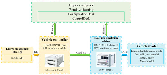
Figure 21.
Overall framework diagram of the experimental bench.

Figure 22.
Diagram of the experimental bench.
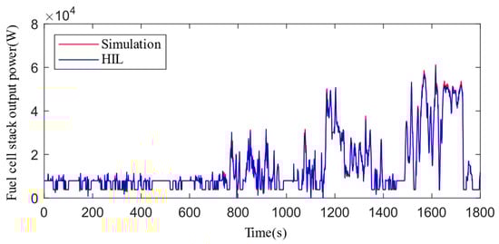
Figure 23.
Fuel cell stack output power in simulation and hardware-in-the-loop (HIL) test.
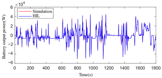
Figure 24.
Battery output power in simulation and hardware-in-the-loop (HIL) test.
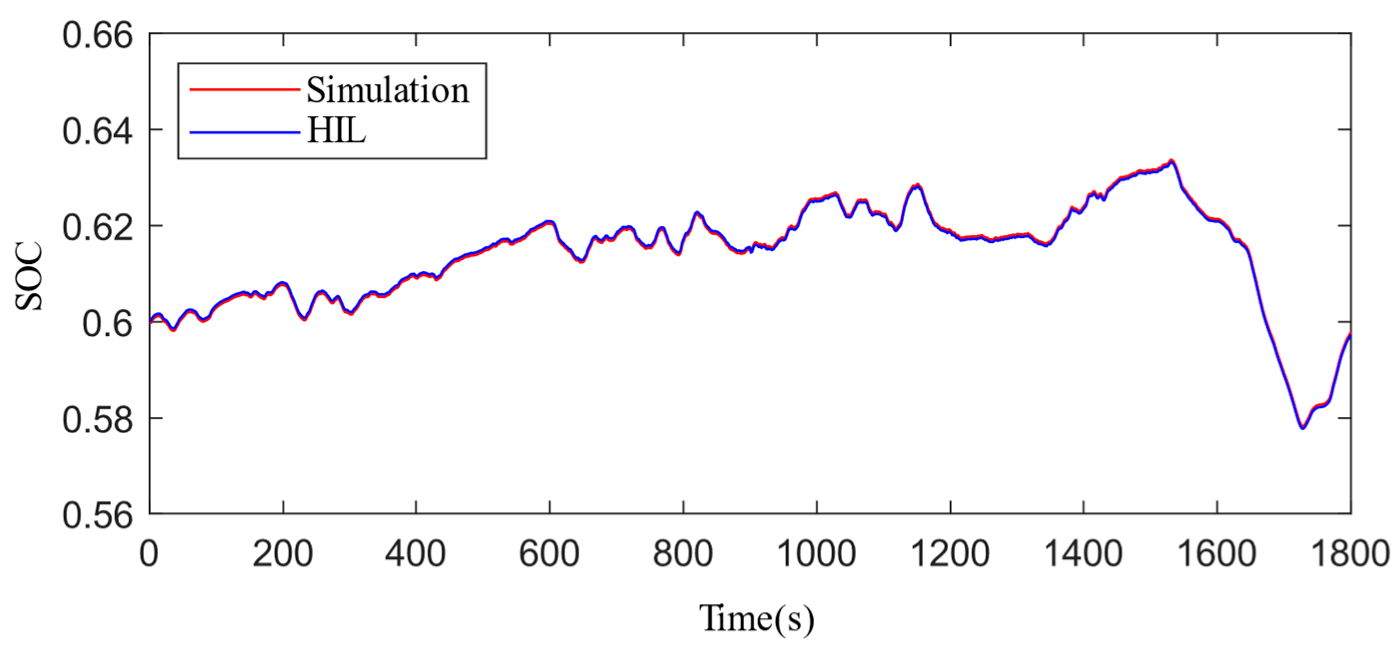
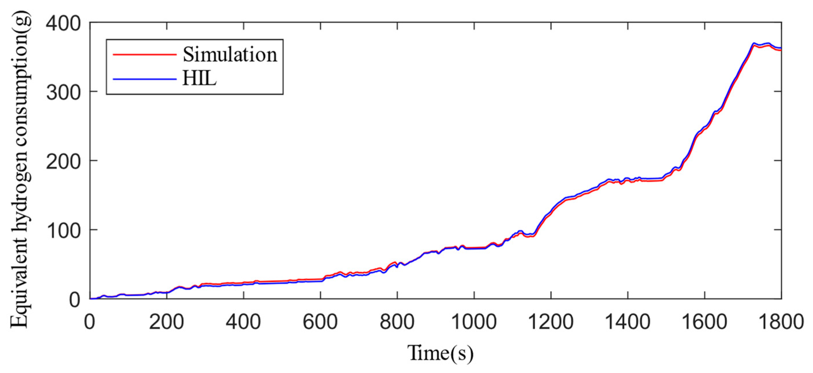
As shown in Figure 25, the trends and fluctuations of the battery SOC trajectory in the simulation and HIL test were similar, with very small errors. The final SOC was close to about 0.6, which confirmed that the adopted strategy could effectively maintain the battery charge stability and adapt to the real vehicle environment. The equivalent hydrogen consumption of the DA-ECMS in the HIL test was 361.9 g, as shown in Figure 26, which was only 2.4 g higher than the simulation results. Its trajectory was almost the same as the simulation trajectory, which indicated that the strategy could also maintain good economy in a real vehicle environment.
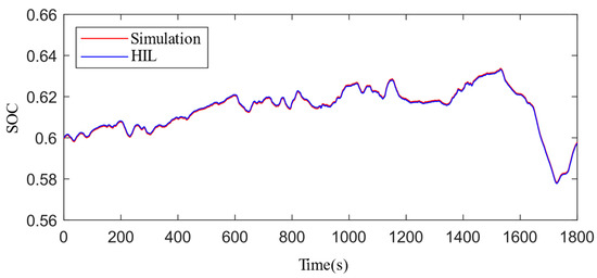
Figure 25.
SOC trajectories from simulation and HIL test.
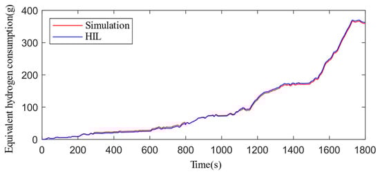
Figure 26.
Equivalent hydrogen consumption of DA-ECMS in simulation and HIL test.
6. Conclusions
The optimal covariate predictor and DA-ECMS are proposed in this paper. First, two indicators—namely the fuel cell stack voltage and the battery capacity—were selected to characterize the performance degradation of the hybrid energy sources, and a corresponding performance degradation model was constructed. Second, a speed prediction model was constructed based on the LSTM neural network, and an optimal covariate predictor was created based on the PMP. The prediction accuracies of the predictor model were 91.44% and 88.17% under the WLTP and CLTC, respectively. The fuel cell and battery performance degradation were then incorporated into the optimization objective of the A-ECMS to construct a DA-ECMS. Compared with the A-ECMS, the DA-ECMS achieved reductions in the fuel cell stack voltage degradation of 17.1%, 23.2%, and 16.6% under the WLTP, CLTC, and NEDC conditions, respectively, and the corresponding battery capacity degradation reductions were 5.1%, 11.1%, and 11.2%. In comparison with the A-ECMS, this sacrifice under the DA-ECMS was relatively small in terms of economy, despite the slight increases in the hydrogen consumption over 100 km of 2.7%, 6.6%, and 9.1%, respectively. Finally, the DA-ECMS was validated by HIL tests. Compared with the simulation, the fuel cell stack voltage degradation, the battery capacity degradation, and the 100-km hydrogen consumption of this strategy under WLTP conditions only increased by 4.5%, 2.7%, and 0.4%, which is within an acceptable error range. Therefore, the EMS established in this paper has good effectiveness and real-time performance capabilities. In the future, the prediction of optimal covariates will be performed using other neural networks and tested on real vehicles.
Author Contributions
Methodology, C.D.; Software, Y.W. and H.D.; Validation, Y.W. and H.D.; Formal analysis, Y.W.; Data curation, H.D.; Writing—original draft, P.Z. and Y.W.; Writing—review & editing, P.Z. and C.D.; Supervision, P.Z. and C.D.; Funding acquisition, P.Z. and C.D. All authors have read and agreed to the published version of the manuscript.
Funding
This work was supported by the National Natural Science Foundation of China (52305069), Foshan Xianhu Laboratory of the Advanced Energy Science and Technology Guangdong Laboratory (XHRD2024-11233100-01), Key R&D project of Hubei Province, China (2021AAA006).
Data Availability Statement
The raw data supporting the conclusions of this article will be made available by the authors on request.
Conflicts of Interest
The authors declare no conflict of interest.
List of Nomenclature
| FCHEV | fuel cell hybrid electric vehicle | activation energy | |
| EMS | energy management strategy | temperature in Celsius | |
| ECMS | equivalent consumption minimization strategy | Ah | Ah-throughput |
| PEMFC | proton exchange membrane fuel cell | power law factor | |
| LSTM | long short-term memory | SOC-related coefficient | |
| SOC | state of charge | SOC-related coefficient | |
| traction force | charge/discharge rate | ||
| f | rolling resistance coefficient | motor power | |
| m | mass of FCHEV | motor torque | |
| angle of road slope | motor speed | ||
| A | frontal area | motor efficiency | |
| CD | drag coefficient | fuel cell instantaneous hydrogen consumption | |
| vehicle rotational mass conversion coefficient | power demand | ||
| velocity | B | pre-exponential factor | |
| g | gravitational constant | battery hydrogen consumption | |
| powertrain power demand | covariate | ||
| fuel cell stack output power | current | ||
| output power of battery | equivalence factor | ||
| unidirectional DC/DC converter efficiency | R | internal resistance | |
| bidirectional DC/DC converter efficiency | degradation loss voltage | ||
| single fuel cell output voltage | activation loss | ||
| theoretical thermodynamic electric potential | ohmic loss | ||
| reference potential per unit of activity | concentration loss | ||
| other component power loss | F | Faraday constant | |
| fuel cell hydrogen consumption rate | R0 | gas molar constant | |
| hydrogen molar mass | P | total pressure in pile | |
| LHV | hydrogen low heating value | partial pressure of hydrogen | |
| voltage degradation of single fuel cell | partial pressure of oxygen | ||
| battery instantaneous consumption rate | partial pressure of water vapor | ||
| battery output power | fuel cell stack output power | ||
| instantaneous total hydrogen consumption rate | N | number of single cells | |
| open-circuit voltage | single cell current | ||
| fuel cell instantaneous hydrogen consumption rate | fuel cell system net output power | ||
| air compressor power loss | |||
| initial value of SOC | battery capacity loss | ||
| nominal battery capacity |
References
- Olabi, A.G.; Wilberforce, T.; Abdelkareem, M.A. Fuel cell application in the automotive industry and future perspective. Energy 2021, 214, 118955. [Google Scholar] [CrossRef]
- Ramadhani, F.; Hussain, M.A.; Mokhlis, H.; Fazly, M.; Ali, J.M. Evaluation of solid oxide fuel cell based polygeneration system in residential areas integrating with electric charging and hydrogen fueling stations for vehicles. Appl. Energy 2019, 238, 1373–1388. [Google Scholar] [CrossRef]
- Chen, K.; Laghrouche, S.; Djerdir, A. Fuel cell health prognosis using unscented Kalman filter, postal fuel cell electric vehicles case study. Int. J. Hydrogen Energy 2019, 44, 1930–1939. [Google Scholar] [CrossRef]
- Jia, C.; Zhou, J.; He, H.; Li, J.; Wei, Z.; Li, K.; Shi, M. A novel energy management strategy for hybrid electric bus with fuel cell health and battery thermal-and health-constrained awareness. Energy 2023, 271, 127105. [Google Scholar] [CrossRef]
- Song, D.; Wu, Q.; Yang, D.; Zeng, X.; Qian, Q.; Zhang, X. Research on operation cost minimization online energy management strategy for fuel cell hybrid passenger vehicles. Proceedings of the Institution of Mechanical Engineers, Part D. J. Automob. Eng. 2024, 238, 420–432. [Google Scholar] [CrossRef]
- Yi, F.; Lu, D.; Wang, X.; Pan, C.; Tao, Y.; Zhou, J.; Zhao, C. Energy management strategy for hybrid energy storage electric vehicles based on pontryagin’s minimum principle considering battery degradation. Sustainability 2022, 14, 1214. [Google Scholar] [CrossRef]
- Teng, T.; Zhang, X.; Dong, H.; Xue, Q. A comprehensive review of energy management optimization strategies for fuel cell passenger vehicle. Int. J. Hydrogen Energy 2020, 45, 20293–20303. [Google Scholar] [CrossRef]
- Yue, M.; Jemei, S.; Gouriveau, R.; Zerhouni, N. Review on health-conscious energy management strategies for fuel cell hybrid electric vehicles, Degradation models and strategies. Int. J. Hydrogen Energy 2019, 44, 6844–6861. [Google Scholar] [CrossRef]
- Sulaiman, N.; Hannan, M.A.; Mohamed, A.; Ker, P.J.; Majlan, E.H.; Daud, W.W. Optimization of energy management system for fuel-cell hybrid electric vehicles, Issues and recommendations. Appl. Energy 2018, 228, 2061–2079. [Google Scholar] [CrossRef]
- Mohammed, A.S.; Atnaw, S.M.; Salau, A.O.; Eneh, J.N. Review of optimal sizing and power management strategies for fuel cell/battery/super capacitor hybrid electric vehicles. Energy Rep. 2023, 9, 2213–2228. [Google Scholar] [CrossRef]
- Ganesh, A.H.; Xu, B. A review of reinforcement learning based energy management systems for electrified powertrains, Progress, challenge, and potential solution. Renew. Sustain. Energy Rev. 2022, 154, 111833. [Google Scholar] [CrossRef]
- Chen, B.; Ma, R.; Zhou, Y.; Ma, R.; Jiang, W.; Yang, F. Co-optimization of speed planning and cost-optimal energy management for fuel cell trucks under vehicle-following scenarios. Energy Convers. Manag. 2024, 300, 117914. [Google Scholar] [CrossRef]
- Yang, D.; Wang, L.; Yu, K.; Liang, J. A reinforcement learning-based energy management strategy for fuel cell hybrid vehicle considering real-time velocity prediction. Energy Convers. Manag. 2022, 274, 116453. [Google Scholar] [CrossRef]
- Jouda, B.; Al-Mahasneh, A.J.; Mallouh, M.A. Deep stochastic reinforcement learning-based energy management strategy for fuel cell hybrid electric vehicles. Energy Convers. Manag. 2024, 301, 117973. [Google Scholar] [CrossRef]
- Jia, C.; He, H.; Zhou, J.; Li, J.; Wei, Z.; Li, K. Learning-based model predictive energy management for fuel cell hybrid electric bus with health-aware control. Appl. Energy 2024, 355, 122228. [Google Scholar] [CrossRef]
- Chen, W.; Peng, J.; Chen, J.; Zhou, J.; Wei, Z.; Ma, C. Health-considered energy management strategy for fuel cell hybrid electric vehicle based on improved soft actor critic algorithm adopted with Beta policy. Energy Convers. Manag. 2023, 292, 117362. [Google Scholar] [CrossRef]
- Luo, Y.; Wu, Y.; Li, B.; Qu, J.; Feng, S.P.; Chu, P.K. Optimization and cutting-edge design of fuel-cell hybrid electric vehicles. Int. J. Energy Res. 2021, 45, 18392–18423. [Google Scholar] [CrossRef]
- Sorlei, I.S.; Bizon, N.; Thounthong, P.; Varlam, M.; Carcadea, E.; Culcer, M.; Iliescu, M.; Raceanu, M. Fuel cell electric vehicles—A brief review of current topologies and energy management strategies. Energies 2021, 14, 252. [Google Scholar] [CrossRef]
- Zhao, X.; Wang, L.; Zhou, Y.; Pan, B.; Wang, R.; Wang, L.; Yan, X. Energy management strategies for fuel cell hybrid electric vehicles, Classification, comparison, and outlook. Energy Convers. Manag. 2022, 270, 116179. [Google Scholar] [CrossRef]
- Zhang, Y.; Chen, M.; Cai, S.; Hou, S.; Yin, H.; Gao, J. An online energy management strategy for fuel cell hybrid vehicles. In Proceedings of the 2021 40th Chinese Control Conference (CCC), Shanghai, China, 26–28 July 2021; pp. 6034–6039. [Google Scholar]
- Li, H.; Ravey, A.; N’Diaye, A.; Djerdir, A. Online adaptive equivalent consumption minimization strategy for fuel cell hybrid electric vehicle considering power sources degradation. Energy Convers. Manag. 2019, 192, 133–149. [Google Scholar] [CrossRef]
- Chen, J.; He, H.; Quan, S.; Zhang, Z.; Han, R. Adaptive energy management for fuel cell hybrid power system with power slope constraint and variable horizon speed prediction. Int. J. Hydrogen Energy 2023, 48, 16392–16405. [Google Scholar] [CrossRef]
- Vignesh, R.; Ashok, B. Intelligent energy management through neuro-fuzzy based adaptive ECMS approach for an optimal battery utilization in plugin parallel hybrid electric vehicle. Energy Convers. Manag. 2023, 280, 116792. [Google Scholar] [CrossRef]
- Piras, M.; De Bellis, V.; Malfi, E.; Novella, R.; Lopez-Juarez, M. Hydrogen consumption and durability assessment of fuel cell vehicles in realistic driving. Appl. Energy 2024, 358, 122559. [Google Scholar] [CrossRef]
- Piras, M.; De Bellis, V.; Malfi, E.; Novella, R.; Lopez-Juarez, M. Adaptive ECMS based on speed forecasting for the control of a heavy-duty fuel cell vehicle for real-world driving. Energy Convers. Manag. 2023, 289, 117178. [Google Scholar] [CrossRef]
- Zhou, B.; Burl, J.B.; Rezaei, A. Equivalent consumption minimization strategy with consideration of battery aging for parallel hybrid electric vehicles. IEEE Access 2020, 8, 204770–204781. [Google Scholar] [CrossRef]
- He, K.; Qin, D.; Chen, J.; Wang, T.; Wu, H.; Wang, P. Adaptive equivalent consumption minimization strategy for fuel cell buses based on driving style recognition. Sustainability 2023, 15, 7781. [Google Scholar] [CrossRef]
- Sahwal, C.P.; Sengupta, S.; Dinh, T.Q. Advanced equivalent consumption minimization strategy for fuel cell hybrid electric vehicles. J. Clean. Prod. 2024, 437, 140366. [Google Scholar] [CrossRef]
- Qi, Y.; Espinoza-Andaluz, M.; Thern, M.; Li, T.; Andersson, M. Dynamic modelling and controlling strategy of polymer electrolyte fuel cells. Int. J. Hydrogen Energy 2020, 45, 29718–29729. [Google Scholar] [CrossRef]
- Huang, Y.; Hu, H.; Tan, J.; Lu, C.; Xuan, D. Deep reinforcement learning based energy management strategy for range extend fuel cell hybrid electric vehicle. Energy Convers. Manag. 2023, 277, 116678. [Google Scholar] [CrossRef]
- Pei, P.; Chang, Q.; Tang, T. A quick evaluating method for automotive fuel cell lifetime. Int. J. Hydrogen Energy 2008, 33, 3829–3836. [Google Scholar] [CrossRef]
- Li, K.; Zhou, J.; Jia, C.; Yi, F.; Zhang, C. Energy sources durability energy management for fuel cell hybrid electric bus based on deep reinforcement learning considering future terrain information. Int. J. Hydrogen Energy 2024, 52, 821–833. [Google Scholar] [CrossRef]
- Ye, Y.; Wang, H.; Xu, B.; Zhang, J. An imitation learning-based energy management strategy for electric vehicles considering battery aging. Energy 2023, 283, 128537. [Google Scholar] [CrossRef]
- Gharibeh, H.F.; Yazdankhah, A.S.; Azizian, M.R. Energy management of fuel cell electric vehicles based on working condition identification of energy storage systems, vehicle driving performance, and dynamic power factor. J. Energy Storage 2020, 31, 101760. [Google Scholar] [CrossRef]


Disclaimer/Publisher’s Note: The statements, opinions and data contained in all publications are solely those of the individual author(s) and contributor(s) and not of MDPI and/or the editor(s). MDPI and/or the editor(s) disclaim responsibility for any injury to people or property resulting from any ideas, methods, instructions or products referred to in the content. |
© 2024 by the authors. Licensee MDPI, Basel, Switzerland. This article is an open access article distributed under the terms and conditions of the Creative Commons Attribution (CC BY) license (https://creativecommons.org/licenses/by/4.0/).