Abstract
The continuous improvement of bridge construction technology has resulted in an ongoing expansion of bridge spans, which has concomitantly increased the difficulty of controlling the alignment of long-span bridges during construction. In order to address the issue of the grey prediction model exhibiting a significant discrepancy in its alignment predictions for long-span continuous girder bridges, a pre-camber prediction method for bridges based on a combination of the grey model (GM) and BP neural network (GM-BP) is proposed. Firstly, the parameters are identified according to their influence on the pre-camber, and the appropriate parameters are selected as the original data to improve the efficiency of prediction. Subsequently, the original data are preliminarily fitted by the GM(1,1) model, and the predicted values are used as inputs for training the neural network. Finally, the new predicted values are output using the nonlinear fitting ability of the BP neural network. To assess the efficacy of the model, it is applied to the prediction of the pre-camber of the girder segments of a bridge under cantilever construction. The pre-camber prediction for 11#–13# girder sections was based on 10 sets of monitoring data from constructed girder sections. The results demonstrated that the average relative error of the GM-BP combined prediction model was 3.01%, which was 5.68% less than that of the GM(1,1) model, and the overall prediction exhibited a closer alignment with the original data. The GM-BP combined prediction model is an effective method for ensuring the alignment control of bridge construction and is able to achieve high accuracy and stability in its predictions in the case of limited and irregular data.
1. Introduction
With the improvement of construction technology, engineering materials, and construction equipment, the construction speed and scale of bridges continues to climb, generating significant economic benefits. However, this expansion in bridge spans has also given rise to a range of challenges [1]. The structural form of a bridge project tends to be increasingly complex. The line control of a large-span bridge during the construction process is also more and more difficult. To ensure that the bridge line meets design requirements, it is necessary to take scientific and reasonable control measures. Bridges are intricate systems, and the control of their structural compliance with design requirements is critical to their verification testing and monitoring [2]. Pre-camber, as an important parameter in the process of the cantilever construction of long-span continuous girder bridges, refers to the amount of correction in the opposite direction of the displacement reserved in the construction or manufacturing process in order to offset the deflection of girders, arches, trusses, and other structures under the action of loads. The improvement of its prediction accuracy is of great significance to ensure that the line shape during the construction stage and the state of bridge completion meet the design requirements.
Currently, common line prediction methods are divided into two main categories: the first is cybernetic models based on less data and poor information, represented by grey model theory; the second is probabilistic and stochastic process models based on big data and multiple samples, represented by Kalman filtering [3] and the neural network method [4]. The grey system theory [5] was proposed by Professor Deng Julong in China in 1982. During the 1990s, grey system theory began to be applied in the field of bridge construction control and was accepted by a large number of experts and scholars. Gao Liangliang [6] used the traditional GM(1,1) model to predict the pre-camber of each girder section of the Beijing Ring Road Special Bridge, and after comparison with the measured values, the results show that this model is more effective for bridge alignment control. Zhang Xiedong et al. [7] applied the metabolic GM(1,1) model for a temperature deflection prediction of the Stirrup Kou Yellow River Special Bridge in Baotou, Inner Mongolia, and found that the accuracy of the model is high, while its method is simple and reliable, making it possible to correct the effect of temperature change on the control of the bridge’s construction alignment in a timely manner. Yao Rong [8] used the GM(1,1) model with four- and six-sample data to predict the value of formwork elevation in real projects, and the results showed that the increase in sample data did not significantly improve the accuracy; then, the GM(1,1) and GM(2,1) models with the same four-sample data were compared and analysed, and it was discovered that the original data matched with a reasonable number of orders in order to better improve the accuracy of the prediction. Bao Yijun et al. [9] corrected the background and initial values of the GM(1,1) model, and the improved prediction results of the model are in good agreement with the actual line shape, which means the model can be stably applied to the cantilever construction control of large-span bridges. Bao Longsheng et al. [10] improved the grey theory based on the cumulative method and used the enhanced grey prediction model to predict the elevation of the Dandong Shuanggang Bridge in Liaoning, which optimised the average relative error from 0.044% to 0.033%. Hong Xiaojiang et al. [11] carried out a double optimisation of the order and background value of the GM(1,1) model, established a fractional-order GM(1,1) model based on Newton’s quadratic interpolation, and applied it to the prediction of the pre-camber of the Litou River Bridge. The results indicated that its prediction accuracy was significantly better than the traditional and fractional-order GM(1,1) models, and it had a certain degree of operability. Liu Laijun et al. [12] estimated the parameters of the GM(1,1) model from the perspective of linear programming, and it was verified that it could better solve the problem of unstable data and increase the stability of the linear prediction of bridges.
In recent years, with the development of science and technology, artificial intelligence technology, represented by artificial neural networks, has been gradually applied to the field of bridge construction; the BP neural network [13] is widely used in bridge construction monitoring and prediction due to its strong nonlinear fitting ability and adaptive ability. Yang Lei et al. [14] used a BP neural network model to identify the key parameters of the Jialing River Bridge and predicted and adjusted its subsequent sections based on the elevation data available under its current construction status, which ensured smooth construction and accuracy control. Yu Jingfei et al. [15] established a BP neural network prediction model based on particle swarm optimisation, based on which the correction value of the elevation of the standing mould was predicted and a more ideal bridge formation was obtained, which provided a reference for the linear control of the main girders of cable-stayed bridges. Zhang X. F. [16] established a BP neural network prediction model to predict the deflection of the main girder using the monitoring data of a bridge’s construction, and the results show that the predicted value is close to the measured value, meeting the requirements of the construction control of cable-stayed bridges. Zhang Jiaxian [17] proposed a bi-level control method for main girder alignment based on parameter identification and alignment deviation prediction for the alignment control of a continuous girder–arch combination bridge construction on the Taipu River, and the results showed that this method is closer to the actual value than the traditional orthotropic inverted dismantling method. Hailong Zhang et al. [18] combined both a BP neural network and genetic algorithm to predict and control the construction process of the Danjiangkou Second Bridge, which successfully identified the elevation errors caused by the loss of concrete capacity, the modulus of elasticity, and prestress. Liang Dong et al. [19] used the grey correlation method and principal component analysis, a golden ratio value-check method, to achieve the optimisation of the input layer and the network layer, therefore improving the accuracy and efficiency of the neural network’s prediction, which can be better applied to construction monitoring. Zheyuan Record et al. [20] proposed a BP neural network agent model (MEC-BP) based on the thinking evolutionary algorithm (MEC) to predict the line shape of the Liangqugou Bridge in Shaanxi Province; the predicted values are in good agreement with the measured values, and it has a stronger generalisation ability than the traditional BP neural network model.
In summary, a large number of studies have been carried out by scholars at home and abroad for the prediction and analysis of bridges’ linear shape. However, most of the proposed bridge alignment prediction methods above are based on a single prediction model or an improved model, which does not take into account the limitations of a single prediction model, thus affecting the prediction accuracy of the algorithm. In this paper, based on a full consideration of the grey prediction model and the BP neural network model, the advantages of the two prediction methods are organically combined to establish the GM-BP combined prediction model. This method is then applied to the linear prediction of a large-span continuous bridge, allowing for the verification of the model’s predictive capabilities and the assurance of the safety of bridge construction.
2. Construction of GM-BP Combined Prediction Model
2.1. Fundamentals of GM-BP Combined Prediction Models
Both the GM(1,1) grey prediction model and the BP neural network prediction model have their own pros and cons. The advantages of the GM(1,1) model are that it requires small samples and less computation, and it has strong applicability; however, it lacks self-organisation and the ability to learn autonomously, and it can only carry out single-parameter predictions, so when there is a large degree of data discretisation or the phenomenon of multi-parameter mutual coupling, its prediction accuracy will be significantly affected. BP neural networks have a strong nonlinear fitting ability and can handle multi-parameter coupling problems, but their modelling requires massive sample data for training to ensure their prediction accuracy. Therefore, it is often difficult to achieve the desired results if only one forecasting method is used. Considering the characteristics of few samples and multi-parameter coupling in the process of controlling the construction line of large continuous girder bridges, the prediction data of the GM(1,1) model are taken as the input of the BP neural network, and the actual pre-camber degree is taken as the output to form a GM-BP combined prediction model, so that the prediction accuracy of the bridge’s pre-camber degree can be improved.
2.2. GM(1,1) Prediction Model
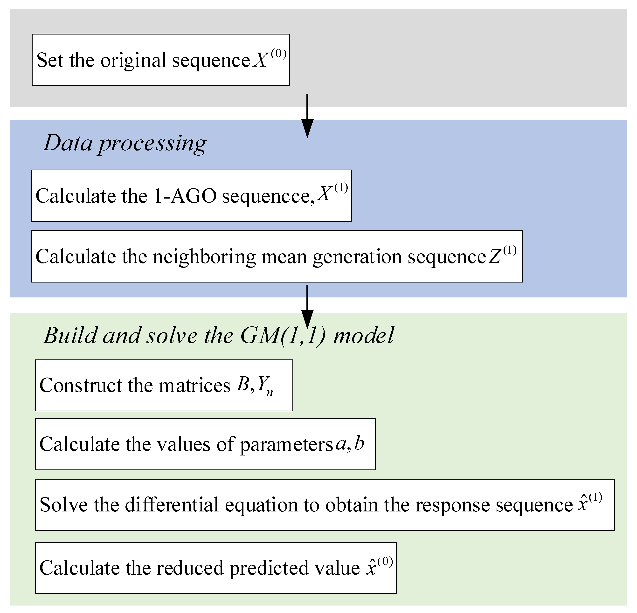
In modelling the GM(1,1) prediction model, it is first necessary to accumulate the original sequence of a given set of data in order to obtain a set of characteristic data sequences exhibiting an obvious trend. The new data sequence is then predicted by solving the parameters, using the least squares method for calculation, and the sequence is subsequently restored using cumulative reduction in order to obtain the predicted result for the original data. The flowchart is shown in Figure 1. The basic modelling steps are as follows:
- (1)
- Let be the original non-negative sequence, defined as follows:
- (2)
- , the 1-AGO sequence, is obtained by accumulating the original sequence once.The value of can be determined by employing the following equation:
- (3)
- Let be the immediate neighbourhood mean generating a sequence of :The value of can be determined by employing the following equation:Thus, the GM(1,1) model can be expressed as follows:The value of the development coefficient () is employed to regulate the developmental dynamics of the system; meanwhile, the grey role quantity () is utilised to reflect the relationship between data changes.
- (4)
- We set , and then the column of the least squares estimated parameters of grey differential Equation (6) is satisfied:where the values of and are as follows:
- (5)
- After obtaining a and b from the least squares estimation, they are substituted into the whitening model of GM(1,1), which is the following:By solving Equation (8), the time response function can be obtained as follows:The time response series of the grey differential equation is as follows:
- (6)
- The above results were cumulated to obtain reduced predicted values:

Figure 1.
Flowchart of GM(1,1) model calculation.
Figure 1.
Flowchart of GM(1,1) model calculation.
2.3. GM-BP Combined Prediction Model
Following the initial prediction by the GM(1,1) model, a BP neural network is employed to train the regression, utilising the initial prediction value as its input. Ultimately, a new prediction value is derived, thereby enhancing the accuracy of the model’s prediction. The flowchart of this is shown in Figure 2. The primary modelling process of the GM-BP combined prediction model is as follows:
- (1)
- A GM(1,1) grey model is fitted to the temperature at the time of measurement, the cantilever gravity, the distance from the tension section to the support, the height of the beam cross-section, the theoretical standing pre-camber, and the actual standing pre-camber to obtain the initial predicted values of these various factors.
- (2)
- In order to enhance the network’s generalisation capacity and the precision of its calculations, while also mitigating the influence of the disparate scales of various factors, this paper employs Equation (12) to normalise the prediction outcomes of the GM(1,1) model.In this equation, represents the normalised data, while and correspond to the maximum and minimum values in each data set, respectively.
- (3)
- The prediction data of the GM(1,1) model are used as the input value of the BP neural network, and the actual standoff pre-camber data are used as the output value to construct the BP neural network model and to adjust the training parameters of the BP neural network, including the maximum number of training times, the learning speed, and the minimum error of training.
- (4)
- The data to be predicted are input into the trained neural network to obtain a normalised predicted value, and finally the normalised predicted value is back-normalised to obtain the predicted elevation.
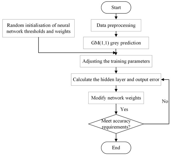
Figure 2.
Flowchart of GM-BP model calculation.
Figure 2.
Flowchart of GM-BP model calculation.
3. Example Application
3.1. Project Examples
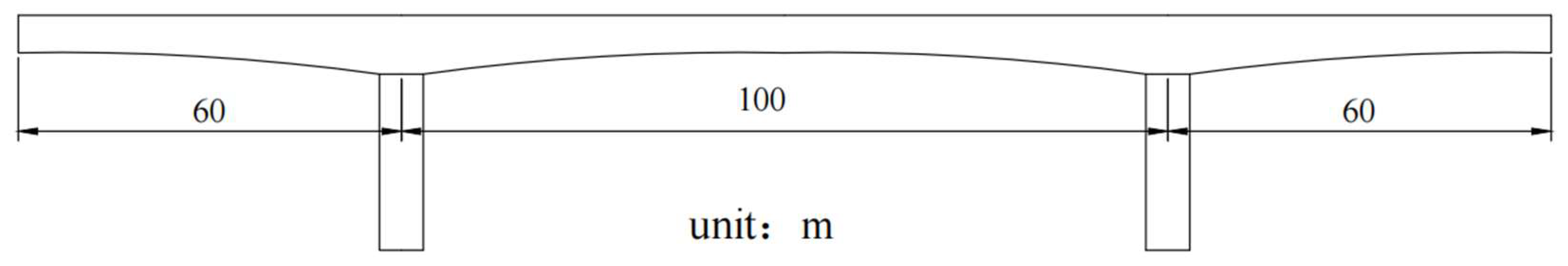
The Tianjin–Qinhuangdao High-Speed Railway construction project, a ballasted track, prestressed concrete, two-row continuous girder bridge, is the engineering example chosen to illustrate a bridge using the cantilever casting method of construction. The total length of the beam is 221.5 m, the calculated span is 60 + 100 + 60 m, the height of the beam at the centre pivot point is 7.85 m, the height of the beam in the 10 m straight section in the middle of the span and the 15.75 m straight section in the side span is 4.85 m, and the bottom edge of the beam is varied according to a quadratic parabola. The schematic diagram is shown in Figure 3.
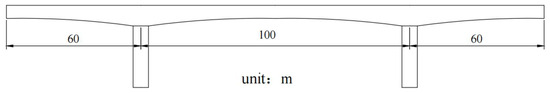
Figure 3.
Schematic diagram of bridge cantilever construction.
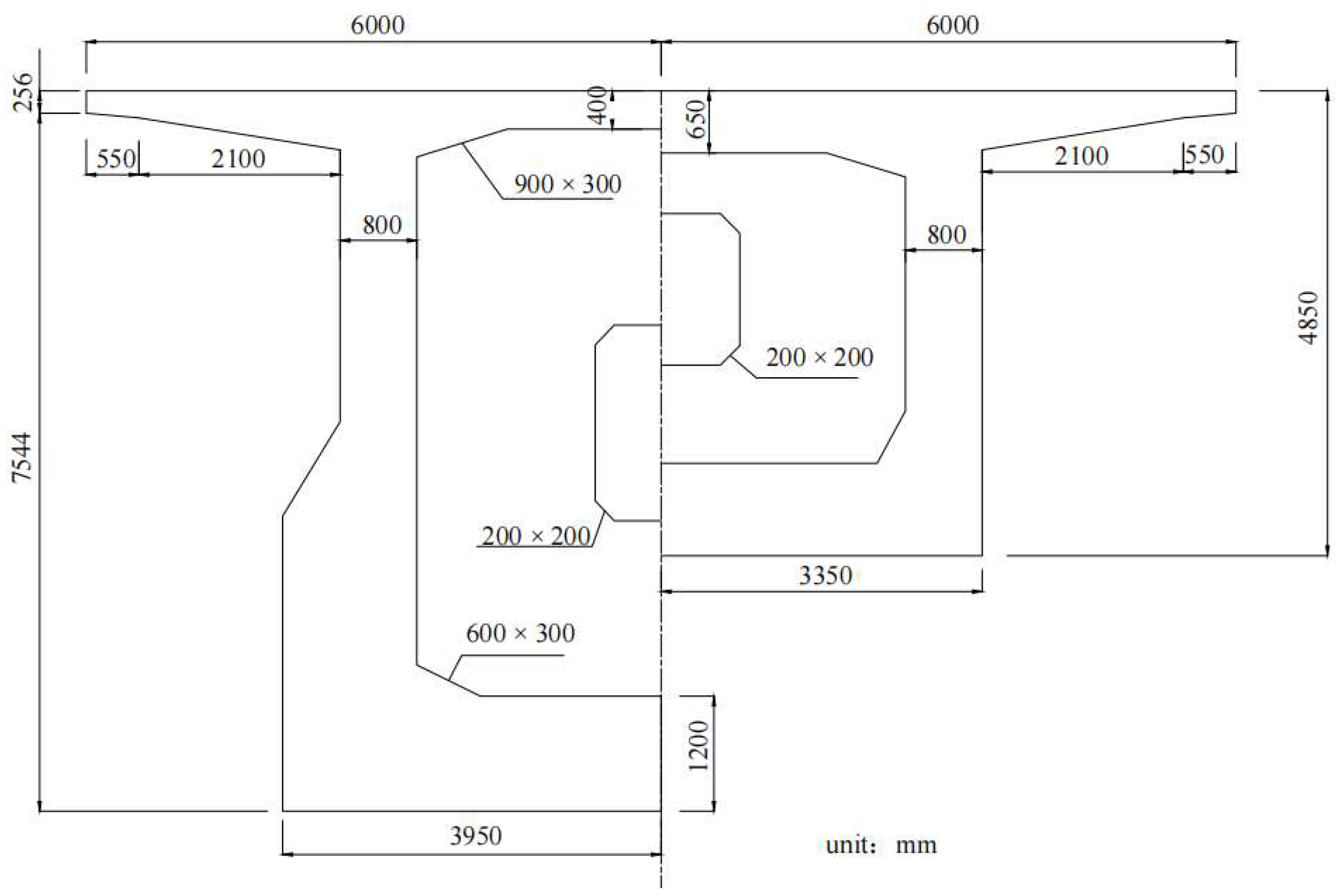
The girder is a single-box, single-compartment, variable-height, variable-section structure. The top width of the box girder is 12.0 m; the bottom width of the box girder is 6.7 m; the thickness of the top plate is 40 cm, except near the end of the girder; the thickness of the bottom plate is from 40 to 120 cm and varies linearly according to a straight line; and the thickness of the web plate is from 60 cm to 80 cm, while the width of the web plate varies from 80 cm to 100 cm according to a folding line, as shown in Figure 4. There are five transverse partitions at the end pivot, mid-span pivot, and centre pivot of the whole girder, and the transverse partitions are equipped with hollows for inspectors to pass through.
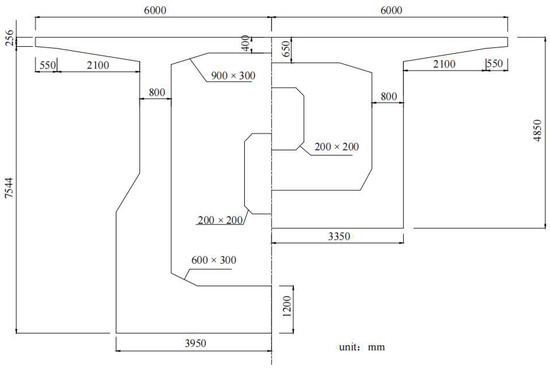
Figure 4.
Bridge bearings and mid-span cross-sections.
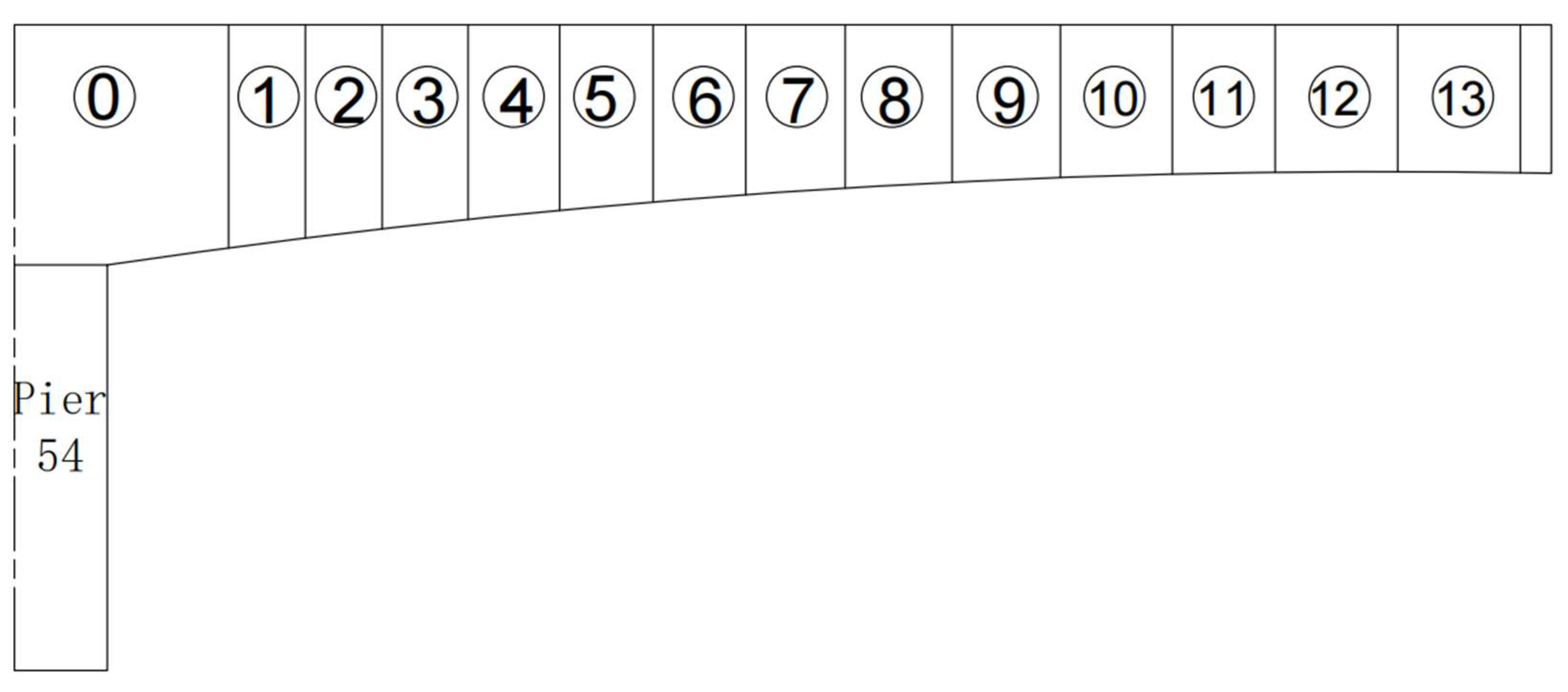
Since the bridge is completely symmetrical, with the mid-span section as the centre, this paper only takes the linear control of cantilever casting towards the mid-span portion of Pier 54 as its example, and its cantilever casting towards the mid-span side is divided into 13 sections, as shown in Figure 5.

Figure 5.
Bridge segmentation chart.
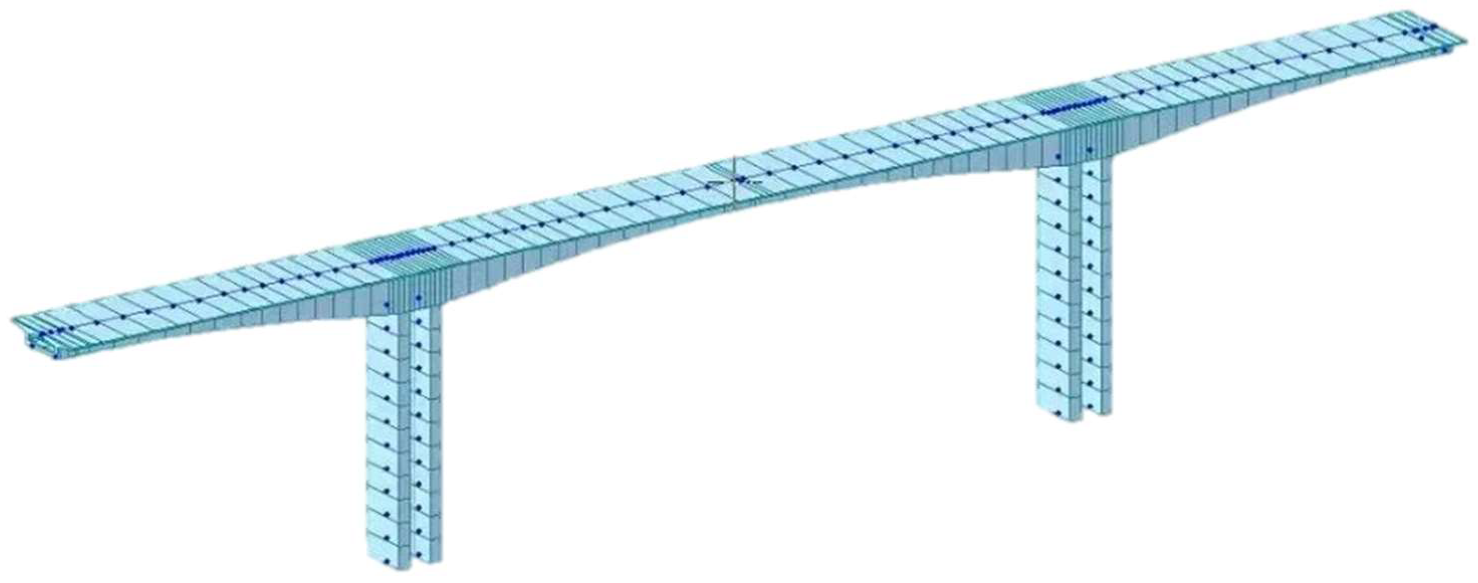
Before using the mathematical model to predict the pre-camber, in order to ensure the smooth progress of the monitoring process, the deformation of the structure needs to be calculated and verified to obtain a theoretical value of the bridge deformation, which, in this paper, is modelled using MIDAS Civil 2021 software. The nodes were divided according to the construction sections of the design drawings, so 16 construction phases were set up, with a total of 86 nodes in the whole bridge, and a rigid connection was adopted between the abutment and Block 0. The established finite element model is shown in Figure 6.

Figure 6.
Finite element model diagram of bridge.
The data were collected during the construction monitoring process and selected as the original data according to their influence on the actual vertical mould’s pre-camber. The original data included the temperature (T, °C), cantilever gravity (G, KN), distance from the tension section to the bearing (L, m), height of the beam cross-section (h, m), the theoretical vertical mould’s pre-camber (f1), and the actual vertical mould’s pre-camber (f2). These original data are presented in Table 1.

Table 1.
Raw construction monitoring data.
3.2. Calculation of the GM(1,1) Prediction Model
Taking the actual standing pre-camber of girder sections 1#–13# in the above table as an example, the sample data of the first 10 girder sections are taken for modelling using the modelling steps in Section 2.2, and the prediction of girder sections 11#–13# is carried out. The main modelling process is as follows:
- (1)
- This is the original sequence of the actual vertical mould’s pre-camber:The 1-AGO sequence is obtained by accumulating the original sequence once:
- (2)
- We solve for the parameters and according to Equation (7), where the matrices and are, respectively, as follows:To obtain and .
- (3)
- Thus, the time response sequence is obtained as follows:
Substituting different values into the cumulative predicted value in turn and then subtracting them through Equation (11) will result in the reduced predicted value.
The remaining sample data were modelled separately following the above steps, and the predictions are shown in Table 2.
Table 2.
Table of GM(1,1) model prediction results.
3.3. Prediction of Pre-Camber by GM-BP Combined Prediction Model
A GM-BP combined prediction model of the pre-camber of a bridge’s vertical mould is established according to Section 2.3, and its main steps are as follows:
- (1)
- The five sets of parameter prediction results of the GM(1,1) model are used as the input parameters of a BP neural network, and the actual vertical mould’s pre-camber is used as the output parameter of the BP neural network, i.e., the number of neurons in the input layer and the output layer of the BP neural network are five and one, respectively, and, after repeated experiments, the training error is minimal when the number of neurons in the implied layer is six. Therefore, in this paper, we establish a three-layer BP with the structure of a 5-6-1 neural network model. The structure of the neural network is shown in Figure 7.
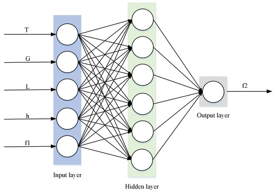 Figure 7. Neural network structure.
 - (2)
- The data from the 1# to 10# beam segments are used as training samples to train the neural network, and the data from the 11# to 13# beam segments are used as test samples to check the predicted values. The data are normalised using Equation (12) to obtain the respective matrices and :
- (3)
- The training parameters of the neural network are set: the maximum number of training iterations is 1000, the learning rate is 0.01, and the network training error accuracy is .
- (4)
- After the training samples are fed into the neural network, the test samples are fed into it for the simulation’s calculation, and the output result is . Then, the predicted value of the pre-camber of the 11#–13# girder segments of the vertical moulds, , can be obtained via the inverse normalisation of the S matrix. Finally, the correlation factors of the remaining girder segments are fed into the trained neural network, and their respective pre-camber predictions are obtained after inverse normalisation.
3.4. Comparative Analysis of Prediction Results
The results of the comparison between the predicted and measured pre-camber values of the two prediction models for the vertical mould pre-camber of the 11#–13# girder sections of the bridge are shown in Table 3. It can be seen that the accuracy of the GM-BP prediction model is more obviously improved compared with that of the GM(1,1) model. Its average relative error is reduced from 8.69% to 3.01%, and the minimum relative error of the GM(1,1) model is 6.38% larger than that of the maximum relative error of the GM-BP model, 4.52%, which indicates that this method can effectively improve the predictions’ accuracy and stability.
Table 3.
Test table of models’ prediction accuracy.
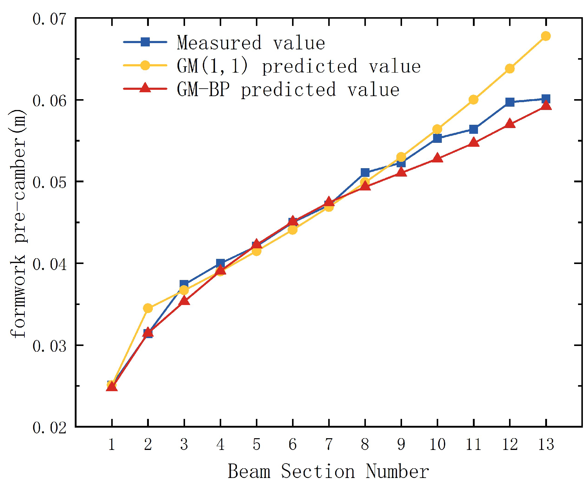
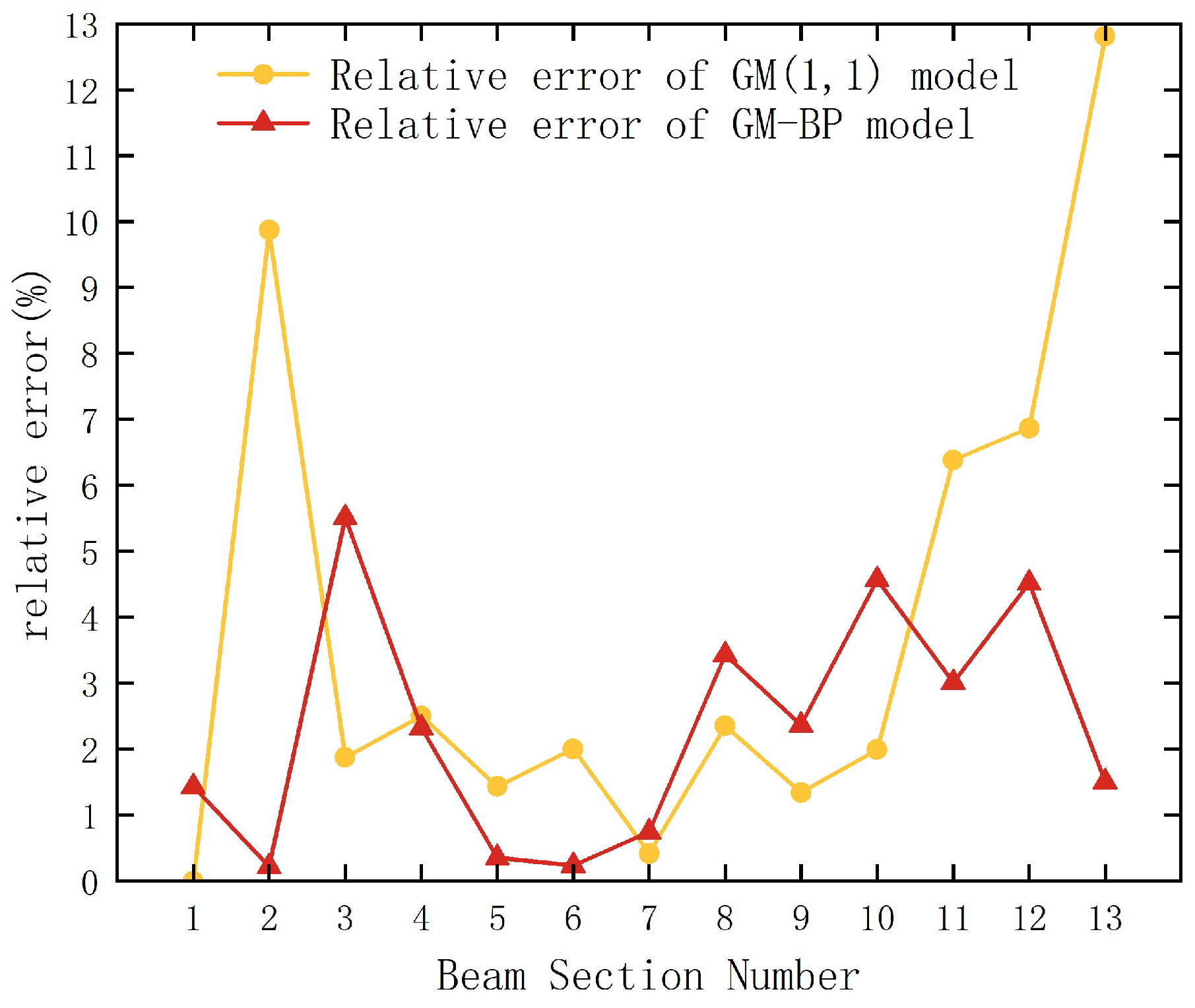
In order to further verify the applicability and accuracy of the model, the predicted values of the pre-camber of the overall girder section were plotted as curves for a comparative analysis with the measured values, as shown in Figure 8 and Figure 9.
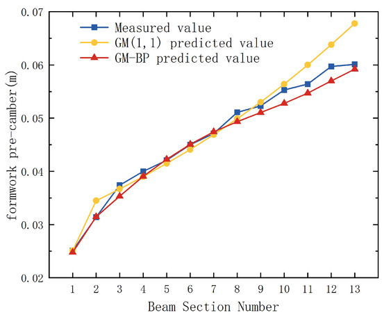
Figure 8.
Comparison chart of model prediction results.
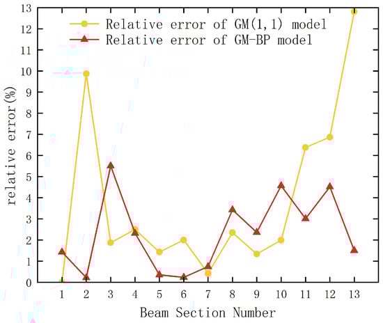
Figure 9.
Comparison chart of relative errors in model predictions.
As can be seen from Figure 8, although both prediction models can truly reflect the variation rule of the pre-camber, the GM(1,1) prediction model has individual girder segments with large errors, especially in the prediction results of the 11#–13# girder segments, which display large discrepancies with the measured values. The GM-BP combined prediction model, on the other hand, demonstrates a high degree of agreement between the predicted and measured values, and there is no significant increase in dispersion. As can be seen from Figure 9, the relative error of the GM(1,1) prediction model fluctuates greatly, and the relative error in the 13# beam section reaches 12.81%, while the fluctuation amplitude of the GM-BP combined prediction model is relatively smooth, and its maximum relative error is 5.51% in the 3# beam section, which is not easily affected by the irregularity of the original data. This shows that the GM-BP combined prediction model can better combine the advantages of the two methods used, can deal with the multi-parameter coupling problem in the case of less data, has a higher accuracy in linear predictions of the bridge construction process, and is more stable.
4. Conclusions
In this paper, the pre-camber seen during bridge cantilever construction is predicted by our established GM-BP combined prediction model, and the main conclusions are as follows:
- (1)
- The GM(1,1) prediction model and the BP neural network model have their own limitations. The prediction accuracy of the former is greatly affected when predicting sample data with a large degree of dispersion; the latter has a better nonlinear fitting ability, but it requires a large amount of sample data, is less stable, and is prone to non-convergence.
- (2)
- The GM-BP combined prediction model can effectively improve prediction accuracy. The prediction result of the GM(1,1) model is used as the input of the BP neural network, and the new prediction value is then output through the neural network, which can give full play to the advantages of the two models: it has the characteristics of requiring fewer samples and having a higher prediction accuracy.
- (3)
- Our validation using engineering examples shows that the GM-BP combined prediction model has significantly improved the prediction accuracy of pre-camber and that the model’s stability is stronger. From the prediction results of the pre-camber of the girder sections 11#-13#, which are to be constructed, compared with those of the GM(1,1) prediction model, the maximum relative error is reduced from 12.81% to 4.52%, and the prediction accuracy is higher; from the prediction results of the whole girder section, the predicted value of the GM-BP model is more in line with the actual value of the pre-camber, and the model’s stability is stronger.
Finally, the performance of the GM-BP combined prediction model largely depends on the choice of its parameter settings. Inappropriate parameter settings may result in suboptimal model performance. Subsequent evaluations and adjustments of the model parameters may be conducted using suitable optimisation algorithms, with the objective of further improving the performance and accuracy of this model.
Author Contributions
Methodology, J.X.; Resources, Q.L.; Writing—original draft, J.X.; Writing—review and editing, Q.L.; Supervision, Q.L. All authors have read and agreed to the published version of the manuscript.
Funding
This research received no external funding.
Institutional Review Board Statement
Not applicable.
Informed Consent Statement
Not applicable.
Data Availability Statement
All the data used in this study can be found in the article.
Conflicts of Interest
The authors declare no conflict of interest.
References
- Zheng, J. Recent Construction Technology Innovations and Practices for Large-Span Arch Bridges in China. J. Eng. 2024, 40, 19. [Google Scholar] [CrossRef]
- Innocenzi, R.D.; Nicoletti, V.; Arezzo, D.; Carbonari, S.; Gara, F.; Dezi, L. A good practice for the proof testing of cable-stayed bridges. J. Appl. Sci. 2022, 12, 3547. [Google Scholar] [CrossRef]
- Yingchun, H. Application of the Kalman′s Filtering Method to the Suspension Bridge Construction Control. J. Highw. Transp. Res. Dev. 1999, 16, 35–38. [Google Scholar]
- Chen, J.; Xiang, M.; Guo, F.; Shen, C. Nerve network method in construction control for long-span bridge. Bridge Constr. 2001, 6, 42–45. [Google Scholar]
- Deng, J. Fundamentals of Grey Theory. Master’s Thesis, Huazhong University of Science and Technology Press, Wuhan, China, 2002. [Google Scholar]
- Gao, L. Application of Grey Theory in Linear Control of Beijing Fourth Ring Special Bridge. Railw. Stand. Des. 2010, 10, 61–63. [Google Scholar]
- Zhang, X.; Xie, L.; Wang, K. Temperature effects in alignment control of continuous concrete girder bridge construction. J. China Foreign Highw. 2010, 5, 36. [Google Scholar]
- Yao, R. Comparison and analysis of grey system prediction model in bridge construction monitoring technology. J. China Foreign Highw. 2011, 31, 160–163. [Google Scholar]
- Bao, Y.; Wang, C.; Zhao, J. Construction control over long-span bridge based on improved grey prediction GM(1,1) model. Railw. Eng. 2016, 18–22. [Google Scholar]
- Bao, L.; Zhou, Z.; Yu, L. Application on GM(1,1) Model Based on Cumulative Method in Bridge Construction Monitoring. J. Shenyang Jianzhu Univ. 2018, 34, 239–246. [Google Scholar]
- Hong, X.; Zhang, X. Application of Optimized Fractional Order GM (1,1) Model inBridge Alignment Control. J. Chongqing Jiaotong Univ. 2022, 41, 65–70. [Google Scholar]
- Liu, L.; Shen, Y. Application of Grey Model based on Linear Programming in Bridge Monitoring. Highway 2021, 66, 101–106. [Google Scholar]
- Rumelhart, D.E.; Hinton, G.E.; Williams, R.J. Learning representations by back-propagating errors. Nature 1986, 323, 533–536. [Google Scholar] [CrossRef]
- Yang, L.; Zhang, Y. Study on the prediction of continuous rigid frame bridge construction geometry control parameter based on neural network theory. Sichuan Build. Sci. 2011, 37, 263–266. [Google Scholar]
- Yu, J.; Wu, Y.; Su, X. Study on predication of line optimization of large-span concrete cable-stayed bridges. J. Railw. Sci. Engineering 2018, 15, 133–140. [Google Scholar]
- Zhang, X.F. The application of BP neural networks in cable-stayed construction control. Appl. Mech. Mater. 2014, 584, 2001–2005. [Google Scholar] [CrossRef]
- Zhang, J. Construction Control Method and Application of Continuous Beam-Arch Combination Bridge Based on Neural Network. Diploma Thesis, Central South University, Changsha, China, 2023. [Google Scholar]
- Zhang, H.; Huang, P.; Tian, W.; Liu, X.; Zhang, P. Analysis of Parameters for Long-span Continuous Bridges Based on Neural Network and Genetic Algorithms. J. Highw. Transp. Res. Dev. 2007, 24, 86–90. [Google Scholar]
- Liang, D.; Chen, H.; Duan, W. Neural network optimization and its application in construction monitoring. J. Hebei Univ. Technol. 2018, 47, 82–89. [Google Scholar]
- Lu, Z.; Wang, X.; Zhao, B. Prediction of construction alignment of long span continuous rigid frame bridge with corrugated steel webs based on MEC-BP surrogate model. J. Chang. Univ. 2021, 41, 53–62. [Google Scholar]

Disclaimer/Publisher’s Note: The statements, opinions and data contained in all publications are solely those of the individual author(s) and contributor(s) and not of MDPI and/or the editor(s). MDPI and/or the editor(s) disclaim responsibility for any injury to people or property resulting from any ideas, methods, instructions or products referred to in the content. |
© 2024 by the authors. Licensee MDPI, Basel, Switzerland. This article is an open access article distributed under the terms and conditions of the Creative Commons Attribution (CC BY) license (https://creativecommons.org/licenses/by/4.0/).