Authenticated Multicast in Tiny Networks via an Extremely Low-Bandwidth Medium

Featured Application

The work may find applications in secure coordination and self-management of groups of unmanned underwater vehicles (UUVs).

Abstract

We consider authenticating multicast messages in the case of extremely narrow communication channels, such as underwater acoustic communication, with devices such as mobile sensors creating a self-organizing autonomous network. Channel characteristics in this scenario prevent the application of digital signatures (and asymmetric cryptography in general), as it would consume too much of the available bandwidth. As communication is relatively sparse, standard symmetric methods such as TESLA have limited application in this scenario as well. Driven by real-world requirements, we focus on tiny networks of only a few nodes. This paper discusses two issues: (a) strategies of key predistribution enabling flexible creation of multicast groups; (b) authenticating multicast messages in a way that prevents an attacker impersonating the sender by subverting one or more receiver nodes and learning the symmetric keys stored by these nodes. For tiny networks, we show that scalable and asymptotically efficient solutions might be useless, and that specially tailored combinatorial approaches may confer some advantage.

1. Introduction

Designing systems composed of autonomous units that can coordinate their activities will likely be the next step in the IoT technological revolution. Progress is conditioned on the availability of reliable communication between the nodes of such a system. In most cases, advanced wireless communication infrastructure (5G and beyond) provides sufficient communication bandwidth with negligible overhead for securing communications with standard cryptographic tools (such as message authentication codes and digital signatures). In addition, the computational effort needed to perform cryptographic operations is acceptable thanks to advances in computational power and dedicated embedded hardware support.

1.1. Problematic Communication Channels

In certain application cases, the target network may be unable to use a reliable and fast communication channel. The main example of such situations involve underwater networks of unmanned underwater vehicles (UUVs) coordinating missions at sea without cable connection (see Figure 1 and Figure 2). As the radio channel is unavailable in this case, the standard option is to use an acoustic channel. From now on, we focus on networks of UUVs as a reference model for our considerations.

Unfortunately, acoustic underwater communication is substantially slower and less reliable compared to radio communication over the air.

Table 1. Selected communication systems based on DPSK (Differential Phase Shift Keying) modulation in shallow and deep water (cf. [1]).

Data Rate (bps)	Bandwidth/ Carrier (kHz)	Bandwidth Efficiency (bps/Hz)	Range (km)	Shallow/Deep
1600	10/50	0.16	0.1	shallow
16,000	8/20	2.0	6.5	deep
20,000	10/50	2.0	1.0	deep

provides example acoustic channel characteristics. Note that the most important application case is communication in shallow water, where the data rate is the lowest and where additional factors degrading the channel performance are more likely. As can be seen, in this case the physical channel capacity may become a major bottleneck for the network even if there are only a few communicating devices. Thus, the communication framework must be designed very carefully in order to avoid any unnecessary communication overhead on top of the transmitted payload bits.

In many cases, not only is the communication bandwidth low, the error rate is also much higher than typical for radio communication. For example, the Bit Error Rate (BER) for underwater acoustic channels can be greater than ${10}^{-1}$ (cf. [2] and [3], among others). In addition to the need to occasionally retransmit the payload data, this may influence the choice of security mechanisms used to protect the communication channel.

1.2. Tradeoff between Channel Security and Payload Capacity

It has become standard practice to protect communication channels with cryptographic mechanisms; encryption guarantees confidentiality of communication, while message authentication codes and digital signatures protect against message manipulation as well as unintentional changes. In many applications, the confidentiality and integrity of communication are fundamental requirements, necessitating the implementation of the above security measures.

This is the case for the problematic networks mentioned above that suffer from limited communication capability. For example, consider the case of underwater sensors monitoring the environment; it is likely that parties illegally dumping waste into the ocean would be interested in manipulating communications between the sensor nodes in order to falsify reports and hide the source of pollution. Likewise, it is critical to protect underwater networks used for defense and anti-terrorist purposes, such as underwater telecommunication cables, power lines connecting off-shore power plants with the power grid, etc.

In high-capacity communication networks, the major problem is to match the speed of cryptographic computation with the high speed of the communication channel. Decades of research and initiatives, such as NIST competitions for fundamental cryptographic primitives, have resulted in tailored solutions for most applications. (Nonetheless, the rules of the game can change in the post-quantum world, where the primitives of today will be replaced by post-quantum algorithms with much higher space and communication costs). In this case, the communication volume overhead resulting from security mechanisms is negligible; what really counts is processing speed. For reference,

Table 2. Comparison of different message authentication options for a message multicast to $n=5$ receivers.

Method of Message Authentication	Size of the Authentication Component (in bits)
ECDSA signature on a 256-bit curve	512
FALCON 512 post-quantum signature (with parameters for NIST security level 1)	>5000
n authentication tags, each 20-bits long (a separate tag generated for each receiver, probability of a forgery of a single tag: $2^{-20}$)	$n·20=100$

presents the length of cryptographic data for a few message authentication methods. Note that if the communication speed is $300\mathrm{kbps}$ and three nodes transmit within 1 s, then adding ECDSA signatures to their messages means an overhead of only about 5 ms! However, if three sensors in shallow water wish to use the 1 s acoustic communication slot for their three messages, then the three ECDSA signatures would consume nearly the entire slot, leaving almost no room for the payload data.

Asymmetric mechanisms have proven to be extremely useful for protecting information channels thanks to their scalability and the separation of public and private keys.

However, there is a lower bound on the length of key material, this bound faces a rising trend due to the progress of cryptanalytic techniques. This makes asymmetric cryptography infeasible for securing networks with extremely low bandwidth; thus, only symmetric cryptography can be used.

1.3. Communication versus Computational Complexity

If the communication speed is extremely low, then the time needed to run cryptographic algorithms is no longer a bottleneck. IoT processors are very capable in this respect (see, for example, Figures 2 and 3 in [4] for SHA256, SHA3-256, and AES performance on MAX32620, MSP432P401R, and STM32L073RZT6 microcontrollers). Moreover, their functionality can be extended with a cryptographic coprocessor [5,6,7].

Apart from the time cost, there is also the issue of energy consumption. In the case of battery-operated devices deployed in the field (e.g., underwater sensors), recharging or replacing the batteries is difficult or even impossible. On the other hand, energy consumption for a given kind of a physical channel cannot be optimized very much due to the laws of physics. This results in the energy cost for sending a bit being significantly higher than for computing it, even if hard cryptographic functions are concerned. This can be clearly seen in the examples of two publications: in [4], the energy consumed for cryptographic computations was measured in $\mathrm{\mu }\mathrm{J}$ (in fact, the most demanding computations investigated in [4], that is, elliptic curve point multiplication, yield consumption on the level of $\mathrm{m}\mathrm{J})$ or in $\mathrm{n}\mathrm{J}/,$ while in [8] the energy consumed for sending packets was on the order of joules. However, in this case, the energy consumed strongly depends on the distance and frequency of the signal. In [9], more factors impacting the energy consumed for communication are indicated, including temperature and pH value.

1.4. Network Scale

A typical network communication architecture aims for scalability; no matter the size of the network, the same mechanisms should be used to encode the information and secure it. A great example showing the power of such methods are digital signatures; any node holding a public key (of a fixed bit size) can verify that a signed message originates from the owner of the corresponding private key.

In certain situations, such as underwater mobile sensor swarms, the number of network nodes will never be high enough for scalability. Apart from physical congestion, the capacity of communication channel may prevent the creation of networks with a high number of nodes. Depending on the particular application, the network designer may be aware of the upper limit on the number of nodes, and as such may not seek out solutions that are asymptotically optimal, i.e., the solution has to solve the network problem up to a certain network size that is known in advance.

It is known that combinatorial properties might be different for small and large numbers. A property that is asymptotically true for large numbers (that is, for n bigger than some threshold value $n_0$) need not be true for small numbers. This is both a challenge and an opportunity, as algorithms developed for arbitrary problem sizes are typically more elegant and ‘clean’; however, given a limited problem size, there may be room for fine-tuning and optimization. We explore these fine-tuning opportunities in this paper.

1.5. Multicasting and the Problem of Shared Symmetric Keys

As explained above, for the target networks, we are forced to use symmetric cryptography. This is not a challenge when one-to-one links have to be secured. If node A shares a key K exclusively with a node B, then securing the link from A to B is not a problem; a message from A can be encrypted with a standard authenticated encryption algorithm such as ASCON [10], then B can decrypt it and check the message authentication code. If this check succeeds, B becomes convinced that the message comes from somebody that knows K. The only party apart from B to know K is A; thus, B concludes that the message comes from A.

As message authentication codes are recomputed by the recipient and are generated by pseudorandom functions, they can be truncated to save bandwidth. By truncation, the chances of guessing the authentication code by the adversary increases, but may be still sufficiently low (after truncating to, say, 20 bits, the adversary may succeed in guessing a correct code for a manipulated message with probability $2^{-20}$).

In the networks considered in this paper, it might be useful or even necessary to use multicast mode instead of sending a message separately to each intended recipient. In that case, authenticated encryption with a shared key K is not enough to authenticate a message. Assuming that A, B, and C share a key K, where A is the intended sender while B and C are intended recipients, if B receives a message correctly encrypted with K, then they can no longer assume that it comes from A, as party C could also have created it. This may happen if C is malicious or simply subverted by an adversary. We assume that the physical protection of the network nodes is limited and that they may be captured, reprogrammed or cloned, and turned against others.

1.6. Further Operating Environment Details

We consider broadcast networks in which a single communication medium is shared by all participants, direct communication between any pair of nodes is possible, as well as direct multicasting to all nodes within range (a single-hop network). However, we remark that many of our results may be generalized to apply to multi-hop networks as well.

The shared communication channel is assumed to have very low bandwidth, precluding the use of many standard mechanisms. To motivate our threat model, we also assume the channel to have large latency, giving rise to attack vectors exploiting the notable differences between reception times of a broadcast message at different nodes.

A slow and unreliable communication channel creates new opportunities for adversaries. First, missing packet delivery or delay is no longer a symptom of an attack. It might frequently be the case that one node receives a multicast message and another does not. In certain cases, such as the underwater acoustic channel scenario, it may be possible for an adversary to use two colluding nodes connected via an efficient and reliable out-of-band channel (e.g., a cable or a radio connection above the surface) to launch wormhole and sinkhole attacks [11].

Unreliability of the channel further prevents the use of protocols based on delayed disclosure of hash pre-images, such as $\mu$Tesla [12], as an adversary may learn the authenticating piece of information (the pre-image) ahead of the nodes in their vicinity and then successfully impersonate the sender.

1.7. Network Setup: Multicast Groups

Due to the limitations of the operating environment, the ability to perform secure multicast transmission is a significant advantage, and may save bandwidth compared to multiple unicast transfers of the same message to different addressees.

We assume that all network nodes are available for personalization, such as preloading requisite cryptographic material by a single entity before the network is deployed in the target environment. This corresponds to, e.g., military and civilian use of swarms of UUVs. In particular, it may be assumed for the purposes of unicast transmission that for any pair of distinct nodes i and j, there is a symmetric link key $K_{ij}$ that is preloaded on both nodes and unknown to all other nodes. This key establishes a secure link between nodes i and j.

We associate the nodes with integer identifiers; for the most part, we shall think of a fixed designated sender S and consider the set of n receivers with identifiers 1 through n. We denote this set of (potential) receivers with $\mathcal{N}=\{1,\dots ,n\}$. Given this notation, we remark that n link keys must be stored (preloaded) per node. This is not a problem for networks of moderate size due to the availability of low-cost non-volatile memory.

Multicast encryption keys are much harder to preload, as their number is exponential in n and corresponds to the possible subsets of $\mathcal{N}$. Each subset $\mathcal{R}\subseteq \mathcal{N}$ with more than one element is a potential multicast group, and dedicated key material must be available for it. This is bad asymptotically, but also unacceptable for the tiny networks we consider; indeed, for a single sender and 20 potential receivers, each receiver already belongs to $2^{19}-1$ multicast groups. Thus, for 256-bit keys (128-bit security level against quantum adversaries), each node would have to store $\approx 16\mathrm{MB}$.

As already mentioned, multicasting is complicated due to the key management and group setup as well as to the problem of source (sender) authentication. In the case of one-to-one communication using link keys, authentication is implicit. If a node j successfully decrypts a message using $K_{ij}$ (we assume authentication encryption), the recipient can be certain that it originated from the node i. For multicasting, this argument does not work, and additional mechanisms must be designed.

1.8. Node Subversion Threat: Impact on Multicast Groups

Because the networks we consider are deployed in a hostile environment, the nodes may only be afforded limited physical protection. Unless they are tamper-resistant (typically not the case), we must consider the threat of an adversary capturing a node, obtaining its cryptographic material, and reprogramming it to do their bidding. Even worse, the obtained keys and other cryptographic material may be loaded onto a more capable device that will work as a clone posing as the captured node in the network. This may be, e.g., a device with a stronger transceiver module that is powered externally or capable of carrying out a wormhole attack.

Given this threat, we make a distinction between internal and external adversaries. An internal adversary is one that has gained access to the cryptographic material (keys) of at least one network node (Figure 3). An attack by an internal adversary corresponds to the scenario described above, where a node is captured and turned against the network. (It may also correspond to successful cryptanalytic efforts by an adversary to learn the keys. Assuming strong cryptographic primitives, this scenario may have a negligible probability.) On the other hand, an external adversary is one that has no access to the keys used by the network nodes. In both cases, we assume that the adversary acts as a man in the middle; they may delete or modify any message sent by node i to node j independently for each pair $(i,j)$, as well as send arbitrary messages to any node i. We naturally extend the notation of internal and external adversaries to multicast groups. For a multicast group $\mathcal{R}$, we say that an adversary is internal if they have compromised one of the receivers in $\mathcal{R}$ (the case of a compromised sender is beyond the scope of this work) and external otherwise, even if they know the keys of other nodes outside the group.

2. Problem Statement

Problem 1.

For tiny networks with a very narrow communication channel, we seek to address the following problems:

1. 

How can the shared keys between the sender and multicast group members be derived without resorting to asymmetric methods such as Diffie–Hellman key exchange, where the messages are relatively long bit strings?

2. 

In reference to the message authentication mechanism for a multicast group, how can the asymmetry in key knowledge between the sender and the receivers be preserved, as is the case of digital signatures, while keeping the total overhead as small as possible?

The asymmetry mentioned above is crucial when facing an internal adversary threat. Answering the questions posed by Problem 1 is the main objective of this paper.

Our Contribution and Paper Organization

His paper makes the following contributions:

• We provide an optimized scheme for multicast group establishment based on summing smaller receiver sets into larger ones.
• We connect the summing strategy for group establishment to a combinatorics problem of covering designs and conclude that improvements to the above scheme are unlikely.
• We introduce a novel scheme for multicast group establishment based on onion encryption that minimizes the communication overhead.
• We introduce a framework of separating families for studying sender authentication schemes in tiny networks under the assumption of a highly constrained communication channel.
• We provide an efficient sender authentication scheme that fits the above framework to enable tweaking the security level and making different trade-offs based on assumptions about the adversary’s behavior.
• We extend the separating families framework to the setting of two corrupt parties, showing that the problem of sender authentication becomes significantly more difficult.
• We propose security policies that complement the proposed sender authentication scheme, increasing the overall security of the system.

Section 3 describes schemes for group establishment, with Section 3.1.1 introducing an optimized scheme for summing receiver sets, Section 3.1.2 studying potential improvements over this scheme, and Section 3.2 focusing on the onion encryption approach. Section 4 concerns sender authentication. Section 4.1 describes the TESLA protocol and Section 4.2 explains why it is inapplicable to the type of networks we are interested in. Section 4.3 introduces the notion of separating families, while Section 4.4 describes a way to view the separating families framework through the lens of graph theory. Section 4.5 studies the optimal separating families for sizes for group sizes up to 20. In Section 4.6, we provide a practical solution to the sender authentication problem based on the separating families framework. We analyze the security of our construction in Section 4.7. Section 4.8 initiates the study of 2-separating families in the context of protecting sender authenticity in the presence of two corrupt nodes. In Section 4.9, we propose techniques and policies aimed at further increasing the security of networks in a low-bandwidth environment. Section 5 summarizes related work, and we conclude the paper in Section 6.

3. Establishing Group Keys

In this section, we discuss strategies to establish a shared key for a multicast group, given some preloaded cryptographic material. This group key can then be used as a master key to encrypt the multicast traffic in the group and for message authentication, helping to protect against external adversaries. Specifically, for a multicast group $\mathcal{R}$, we want the nodes in $\mathcal{R}$ to obtain a group key K for which it is infeasible to derive K for nodes outside of $\mathcal{R}$.

We study three strategies. The first one is preloading keys for all possible groups in the network.

This naïve solution is a reasonable choice for networks of small size, say, $n=4$; however, it quickly becomes impractical for larger values of n. Indeed, in this case, the sender has to hold $2^n-1-n$ group keys (there are $2^n$ subsets of $\mathcal{N}$; we need not consider the empty set and singleton sets, as these correspond to one-to-one communication for which we already assume we have link keys $K_{ij}$). A receiver i has to hold $2^{n-1}-1$ group keys; for any nonempty $U\subseteq \{1,\dots ,n\}\setminus \left\{i\right\}$, node i needs a group key for $U\cup \left\{i\right\}$.

In the following, we propose a tradeoff where the initial storage (preload) requirements are reduced at the cost of requiring communication to establish K. This is motivated by the observation that out of the exponential number of potential multicast groups considered in the above paragraph, only a few will be eventually used in a real-world use case. We discuss two strategies to realize this tradeoff. Both strategies rely on preloading group keys corresponding to some chosen small family of subsets of $\mathcal{N}$. The first strategy is to take the (small) pre-existing groups and build new ones by taking their unions. Conversely, the second strategy relies on taking intersections of large pre-existing groups.

3.1. Summing Strategies

Suppose that we have a predefined family of subsets of $\mathcal{N}$, say, $S_1,\dots ,S_m\subseteq \mathcal{N}$. Let the corresponding multicast keys $K_1,\dots ,K_m$ be preloaded on S. For node $i\in \mathcal{N}$, the key $K_j$ is preloaded on node i if and only if $i\in S_j$. If an encryption key for the group $\mathcal{R}$ is to be established, the sender S:

1.

Chooses a group key K at random;

2.

Selects a set of w indices I such that $\mathcal{R}={\bigcup }_{i\in I}{S}_i$;

3.

Broadcasts w messages, with the ith message being a ciphertext of K obtained with the key $K_i$, i.e., ${\mathsf{Enc}}_{K_i}\left(K\right)$.

As $\mathcal{R}={\bigcup }_{i\in I}{S}_i$, each node of $\mathcal{R}$ can decrypt at least one message and obtain K, while a node from $\mathcal{N}\setminus \mathcal{R}$ learns nothing about K (assuming that the encryption scheme is semantically secure).

Note that the sets $S_i$ selected by I in this solution need not be disjoint; however, the number of sets should be chosen to be as small as possible in order to minimize the number of messages in the third step. We refer to this strategy as the summing strategy.

3.1.1. Decimating the Power Set

Here, we present a concrete instance of the general summing strategy suggested to us by Marcin Kik: first, we split $\mathcal{N}$ into k disjoint subsets ${\mathcal{N}}_1,\dots ,{\mathcal{N}}_k$, each of cardinality $n/k$. For each ${\mathcal{N}}_i$ and each $Z\subseteq {\mathcal{N}}_i$ such that $\left|Z\right|>1$ (here we consider the keys for non-unicast transmission), we generate a separate key $K_Z$. This key is then preloaded on the sender S and all members of the set Z. Suppose that the sender S wants to create a multicast group $\mathcal{R}$. Then, the sender:

1.

Chooses a key K at random;

2.

Finds the intersection $Z_i={\mathcal{N}}_i\cap \mathcal{R}$ for each $i\le k$;

3.

Broadcasts k messages, with the i-th message being a ciphertext of K obtained with the key $K_{Z_i}$, i.e., ${\mathsf{Enc}}_{K_{Z_i}}\left(K\right)$;

4.

For $Z_i={\mathcal{N}}_i\cap \mathcal{R}$ such that $|Z_i|=1$, the ciphertext of K is send to the only $Z_i$ member via one-to-one channel (unicast transmission).

The number of group keys to be stored by the sender now becomes $k·(2^{n/k}-1-n/k)$, while each receiver has to store only $2^{n/k-1}-1$ group keys. For example, for $n=16$ and $k=4$ the sender would have to store 44 preloaded group keys, while each receiver would only have to store 7 preloaded keys. Including the link keys for one-to-one communication with the sender, the sender would have to store 60 keys altogether. A few further examples are presented in

Table 3. Example number of group keys per node with the method from Section 3.1.1.

Number of Receiver Nodes	k	# Group Keys per Receiver	# Keys Stored by the Sender
8	2	7	22
8	4	1	4
16	2	127	494
16	4	7	44

.

3.1.2. Optimizing the Summing Strategy

We can ask how far it is possible to optimize the selection of the family $\{S_1,\dots ,S_m\}$, given that each group key must be established by at most k multicast messages. Unfortunately, it turns out that finding the optimal choice reduces to a long-studied combinatorial problem. For this problem, solutions have been found only for a few small input values. Below, we go into details.

Let $\mathcal{P}$ be a family of subsets of $\mathcal{N}$ such that for each $\mathcal{R}\in \mathcal{P}$ a key $K_{\mathcal{R}}$ is preloaded to the sender S corresponding to the group $\mathcal{R}$. For simplicity, we shall disregard the distinction between group keys and the one-to-one link keys, and allow $\mathcal{P}$ to contain the keys $K_i$ corresponding to the singletons $\left\{i\right\}\subset \mathcal{N}$. For concreteness, let us assume that S can send only four messages to transport the group key to the group members (that is, in the pseudocode at the beginning of this section, $w\le 4$ for every multicast group).

In the following, we shall find a connection between our optimization problem and an old problem from combinatorics. We start in the following way. First, consider a set $\mathcal{R}$ of at least 5 nodes of $\mathcal{N}$. To transmit the group key to $\mathcal{R}$, we must use at least one set $P\in \mathcal{P}$ of cardinality at least 2. Let us narrow our attention to receiver sets of cardinality exactly 5. Let ${\mathcal{N}}_5={\mathcal{N}}_5\left(n\right)$ denote the family of subsets of $\mathcal{N}$ of cardinality 5.

Let ${\mathcal{P}}^{\prime }$ be a subfamily of $\mathcal{P}$ restricted to subsets of $\mathcal{N}$ of cardinality at most 5. Note that only the sets from ${\mathcal{P}}^{\prime }$ can contribute to establishing a group key for a receiver set $\mathcal{R}\in {\mathcal{N}}_5$.

Lemma 1.

Let ${\mathcal{P}}^{\prime \prime }$ be obtained by reducing each $A\in {\mathcal{P}}^{\prime }$ of cardinality greater than 2 to its randomly chosen 2-element subset. Then, for each $D\in {\mathcal{N}}_5$ there is a family of at most 4 elements of ${\mathcal{P}}^{\prime \prime }$ with union to D.

Proof. 

According to our assumptions, there exist sets $P_1,\dots ,P_u\in \mathcal{P}$, $u\le 4$, such that $D={\bigcup }_{i=1}^u{P}_i$. At least one $P_i$ has cardinality at least 2. There is a 2-element subset B of $P_i$ that belongs to ${\mathcal{P}}^{\prime \prime }$. Finally, $D=B\cup \left\{j_1\right\}\cup \left\{j_2\right\}\cup \left\{j_3\right\}$, where $\{j_1,j_2,j_3\}=D\setminus B$. □

Definition 1.

Let ${\gamma }_5={\gamma }_5\left(n\right)$ be the minimal cardinality of a family $\mathcal{F}$ of 2-element subsets of $\mathcal{N}$ such that for every $G\in {\mathcal{N}}_5$ there exists $A\in \mathcal{F}$ such that $A\subset G$.

Corollary 1.

The family $\mathcal{P}$ contains at least ${\gamma }_5$ elements.

Proof. 

Obviously, $|\mathcal{P}|\ge |{\mathcal{P}}^{\prime }|\ge |{\mathcal{P}}^{\prime \prime }|$ (note that it may happen that $|{\mathcal{P}}^{\prime }|>|{\mathcal{P}}^{\prime \prime }|$, as for two elements of ${\mathcal{P}}^{\prime }$ we may choose the same 2-element set A). Per Lemma 1, ${\mathcal{P}}^{\prime \prime }$ satisfies the conditions from Definition 1; thus, $|{\mathcal{P}}^{\prime \prime }|\ge {\gamma }_5$. □

Now, let us recall the following classic concept from combinatorics [13]:

Definition 2.

A family of k-element subsets of $\{1,2,\dots ,v\}$, called blocks, is a$(v,k,t)$-covering design if each t-element subset of $\{1,2,\dots ,v\}$ is contained in one of the blocks.

The main question studied with regard to covering designs is to construct a $(v,k,t)$-covering design with a small number of blocks. We write $C(v,k,t)$ to denote the smallest possible number of blocks in a $(v,k,t)$-covering design.

The number ${\gamma }_5$ corresponds to a dual problem in which 2-element blocks have to be contained in 5-element sets. However, note that a t-element set A is contained in a k-element set B if and only if the $(n-t)$-element set $\mathcal{N}\setminus A$ is a superset of the $(n-k)$-element set $\mathcal{N}\setminus B$. Thus, we may conclude the following:

Corollary 2.

${\gamma }_5\left(n\right)=C(n,n-2,n-5)$.

Let us consider an example case of $n=16$. Then, per Corollary 2, ${\gamma }_5=C(16,14,11)$. A comprehensive base of known values of C can be found at https://ljcr.dmgordon.org/cover/table.html (accessed on 1 September 2024). Unfortunately, it does not contain the value of $C(16,14,11)$. To obtain a rough approximation, we use the Schönheim inequality [14]:

$$C(t,k,v)\ge \lceil t/k·C(t-1,k-1,v-1)\rceil$$

and the known value $C(13,11,8)=15$ (see https://ljcr.dmgordon.org/cover/show_cover.php?v=13&k=11&t=8, accessed on 1 September 2024):

$$C(16,14,11)\ge ⌈{\displaystyle \frac{16}{14}}·⌈{\displaystyle \frac{15}{13}}·⌈{\displaystyle \frac{14}{12}}·⌈{\displaystyle \frac{13}{11}}·C(13,11,8)⌉⌉⌉⌉=29.$$

Hence, ${\gamma }_5\ge 29$, and we need at least 29 subsets of $\mathcal{N}$ in $\mathcal{P}$ with cardinality at least 2. Together with 16 singleton sets (corresponding to link keys responsible for bilateral communication with the receivers), the sender has to preload at least $29+16=45$ keys. Moreover, what we have done is only a rough estimate of the minimal cardinality of $\mathcal{P}$. On the other hand, recall that the simple strategy from Section 3.1.1 requires 60 keys. Therefore, we may conclude the following.

Conclusion 1.

Achieving a significant improvement over the method presented in Section 3.1.1 might be impossible for the small values of n that we study here; moreover, finding optimal solutions by exhaustive search seems infeasible given the lack of results for the seemingly simpler problem of constructing minimal covering designs.

3.2. Intersection Strategy with Onion Encryption

Instead of building the groups from smaller ones, it is possible to take a top-down approach in which the target group is built as an intersection of larger multicast groups. Again, let $\mathcal{N}=\{1,\dots ,n\}$ be the set of receivers and let S be the designated sender.

During a setup phase, for each $i\le n$, a randomly drawn key $L_i$ is preloaded on S and on all receivers in $\mathcal{N}$ except for node i.

Now, let us describe what happens if a multicast group $\mathcal{R}$ has to be established. If $\mathcal{R}$ is not of the form $\mathcal{N}\setminus \left\{i\right\}$, then for any i a group key has to be determined and deployed by S and the member nodes of $\mathcal{R}$. Let $\mathcal{N}\setminus \mathcal{R}=\{i_1,\dots ,i_k\}$. Then, S:

1.

Chooses a group master key K at random;

2.

Broadcasts the onion ciphertext

$$\mathrm{\Phi }={\mathsf{Enc}}_{L_{i_1}}\left({\mathsf{Enc}}_{L_{i_2}}(\dots {\mathsf{Enc}}_{L_{i_k}}\left(K\right)\dots )\right)$$

(1)

together with an identifier of the set $\mathcal{R}$.

Preferably, $\mathsf{Enc}$ should be format-preserving, that is, the ciphertext should be the same length as the plaintext; note that the group key is now transmitted to the target set of receivers in a single broadcast. Each receiver from the set $\mathcal{R}$ can decrypt $\mathrm{\Phi }$, as it knows all keys $L_i$ for $i\notin \mathcal{R}$, and only those keys are used to create $\mathrm{\Phi }$. If $j\notin \mathcal{R}$, then j cannot remove exactly one “layer” of the encryption, namely one created with the key $L_j$. Thus, if $\mathsf{Enc}$ is semantically secure, node j learns nothing about the group key.

We refer to this strategy as the filtering strategy, as each layer of the onion from expression (1) may be viewed as ‘filtering out’ one node of the network. In this scheme, each receiver stores $n-1$ keys and the sender stores n. The main advantage of this method is reducing the number of broadcast messages transporting a group key to just one message and a reasonable number of preloaded keys! A drawback, however, is weaker resilience to node subversion. Any coalition of two compromised nodes may decrypt $\mathrm{\Phi }$, as each node is missing exactly one key and no two nodes are missing the same key.

There are also a number of differences when two networks join. For the summing strategy, if we agree to double the number of messages to create a multicast group, nothing must be changed on the side of the receivers; only the new sender has to collect the keys from the old senders. Thus, the join operation is relatively easy. In the case of the filtering strategy, all receivers must receive new keys.

4. Sender Authentication

For the purposes of this section, we assume that we have a multicast group with a sender S and a set $\mathcal{R}\subseteq \mathcal{N}$ of r receivers. We study the problem of authenticating the origin of multicast messages; each member of $\mathcal{R}$ must be able to filter out the messages that do not originate from S.

We differentiate between $\mathcal{R}$ and $\mathcal{N}$ in order to take the following into account. Note that a ciphertext can be authenticated in front of a broader set than just the set of nodes that are able to decrypt it, that is, confidentiality of the message can be protected independently from its integrity; one of the methods described in Section 3 can be utilized for this purpose. This allows us to study sender authentication on its own as an orthogonal problem. Initially, for authentication purposes, the nodes can be preloaded with the keys corresponding to a few sets $\mathcal{R}$ determined by the deployment of the nodes.

For flexibility reasons, it is advantageous to include all of $\mathcal{N}$ as one of these sets; in case a new group with receiver set $\mathcal{R}$ must be established, the freshly generated keys for $\mathcal{R}$ can be broadcast by S using encryption, as in Section 3, except authenticated in front of everyone (all of $\mathcal{N}$), or some ${\mathcal{R}}^{\prime }\supset \mathcal{R}$ if there are preloaded keys for ${\mathcal{R}}^{\prime }$. After decrypting the messages, the nodes from $\mathcal{R}$ may switch to the new authentication keys. In Section 4.3, we shall see how much communication volume can be saved if the sender switches from authenticating in front of $\mathcal{N}$ to authenticating in front of a subset $\mathcal{R}$. Nevertheless, the smaller the set of nodes knowing the keys, the more limited the impact of node capture.

We are concerned with the situation where digital signatures of S cannot be used to prove the message origin due to channel bandwidth constraints. Message authentication codes based on a symmetric key K shared by S and the nodes in $\mathcal{R}$ can protect the integrity of the messages against external adversaries, but are unfortunately useless against an internal adversary, as a malicious node can create messages and their authentication codes in the same way as S and send them to selected nodes in $\mathcal{R}$. This may create chaos in network operation.

An additional difficulty is the admissible length of message authentication codes. We assume that there might be a strict upper bound on their length and that the bound might be (much) lower than the length of standard message authentication codes. Thus, we identify two high-level approaches to authenticating the origin of messages when restricted to symmetric cryptography. One is to amortize the cost of sender authentication by chaining messages together with cryptographic commitments. By subsequently opening these commitments, the sender proves that the entire chain of messages originated from the same source. If there is a strong proof of origin for the first message, then all the messages in the chain are authenticated robustly. This is the idea behind the TESLA protocol, explicated in Section 4.1. Another approach is to append authentication tags to each message. These tags rely on some secrets shared between the sender S and specific subsets of receivers $\mathcal{R}$, ensuring that no node from $\mathcal{R}$ could forge all tags. An efficient construction of this kind is proposed in Section 4.3.

4.1. TESLA Protocol

TESLA (Timed Efficient Stream Loss-tolerant Authentication) [15], standardized in [16], is a standard multicast authentication protocol. It is computationally lightweight and uses only symmetric cryptographic algorithms. TESLA replaces asymmetric cryptography with time-delayed disclosure of preimages of a one-way function. This restores the asymmetry between the sender and the receivers.

The keys used by TESLA to authenticate the messages are generated according to the Lamport scheme [17], in which the sender uses a one-way function F, chooses the number ℓ of keys to be generated, and randomly generates the initial seed $s_{\ell }$. Each subsequent value is then generated according to the following formula:

$$s_{i-1}=F\left(s_i\right),\mathrm{for}i=\ell ,\ell -1,\dots ,1.$$

(2)

The final element $s_0$ is then transferred to the intended receivers and properly authenticated. The remaining elements of the chain are disclosed in due time: first $s_1$, then $s_2$, and so on. Each $s_i$, $i=1,2,\dots$, is used as a seed to derive an authentication key $K_i$, that is,

$$K_i=F^{\prime }\left(s_i\right),$$

(3)

where $F^{\prime }$ is another one-way function. The $s_i$ are consumed at regular intervals, called epochs. In the i-th epoch, each message m is accompanied with a tag t;

$$t={\mathsf{MAC}}_{K_i}\left(m\right),$$

(4)

where $\mathsf{MAC}$ is a keyed message authentication code function. A receiver cannot verify the tag t immediately, as it does not yet know the key $K_i$ necessary to recompute t according to (4). The element $s_i$ is published by the sender in epoch $i+d$, where d is a delay parameter. At that moment, i.e., when $s_i$ is revealed, the receiver:

• Checks that $s_i$ satisfies Formula (2) (note that $s_{i-1}$ was revealed in the previous epoch);
• Calculates $K_i$ according to (3);
• Checks that the tags from epoch i satisfy Equation (4).

An extension of TESLA enabling packet authentication without delay d was presented in [12] (Section 3.1). In the extension, the messages are buffered by the sender, meaning that in epoch i the sender must know the messages to be sent in epoch $i+d$.

4.2. Inadequacy of TESLA for Low-Bandwidth High-Latency Communication Media

While TESLA has remarkable advantages, including an elegant and flexible design, its applicability in the particular operating environment (see Section 1.6) is limited. Specifically, the following problems arise:

1.

If messages are asynchronous and not sent at a steady rate (e.g., they are triggered by external events), then certain epochs may pass without any workload messages. However, TESLA requires some technical messages in each epoch to operate properly.

2.

Alternatively, if the epochs are driven not by the clock but by the number of messages sent (e.g., the epoch changes every v messages), then some messages can be left unauthenticated for a long time. On the other hand, when a burst of multicast messages occurs in a short time, the epochs will change quickly. This creates a security risk, discussed in Section 4.2.1.

3.

The length of the clock-driven epoch should be adjusted to variable message delivery delays for different network nodes. Thus, the choice implies either long waits for authentication data or the security risk discussed in Section 4.2.1.

4.

If messages are not known in advance, the immediate packet authentication mentioned above cannot be used. It seems that in the case of a network constrained in terms of communication, the opportunities for the messages to be known d epochs ahead of time will be rare; thus, in most cases the mechanism will not be applicable.

4.2.1. Wormhole Attacks against TESLA

Suppose that the TESLA epochs are shorter than the propagation delay for some receivers located far from the sender, and assume that the authentication delay parameter used in the network is $d=2$. We shall consider an adversary creating a “wormhole” connecting distant nodes, affording them a fast communication channel faster than the regular channel used by legitimate nodes. In the underwater setting, this can be achieved by using surface transmitters connected by cable to the UUVs (see Figure 4). In particular, we suppose that for legitimate nodes the propagation time from one end of this wormhole to the other is more than one epoch.

Assume that the sender has sent some packets very close to the end of epoch i; the adversarial node intercepts the packet and waits until the beginning of epoch $i+2$. The seed $s_i$ is disclosed by the sender, and the node can now change the intercepted message and generate the correct authentication code. The manipulated message is sent through the wormhole channel, catching up to or even overtaking messages from epoch i reaching the destination area. In this way, the adversary may flood an isolated network area with forged messages. Note that the adversary does not have to intercept the original packages, as it is suffices for the malicious node to learn $s_i$ transmitted in the regular way.

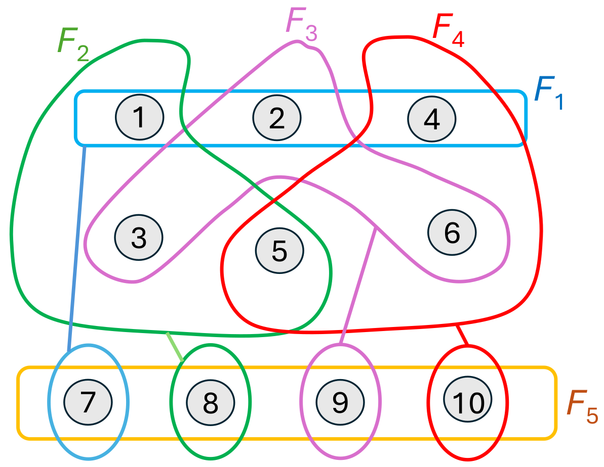
4.3. Separating Families

An alternative to the TESLA protocol is to use multiple authentication tags, with each tag created with a separate key shared by the sender and a different subset of receivers. In this section, we assume that an adversary can compromise at most one node. The other case is discussed in Section 4.8.

For the purposes of this section, we consider a multicast group $\mathcal{R}$. For ease of notation, we assume that $\mathcal{R}=\{1,\dots ,r\}$. We assume that there is a master key K for this group shared by the sender S and all nodes in $\mathcal{R}$. The key K can be used to derive an encryption key for all multicast messages for group $\mathcal{R}$. Moreover, it can be used to create message authentication codes that can be verified (but also forged) by every node in $\mathcal{R}$. In this way, we attempt to protect against an external adversary.

The strategy is to attach not one but k short message authentication tags $t_1,\dots ,t_k$ to each message, where:

• The ith tag $t_i$ is created with a separate symmetric key $K_i$ shared by the sender and a set $F_i$ of receivers $F_i\subseteq \mathcal{R}$;
• A receiver j may verify the i-th tag if and only if it knows $K_i$, i.e., $j\in F_i$.

The details of how the tags are created are described in Section 4.6. For now, the key point is that if a node j knows $K_i$, then it can both verify and create a valid tag $t_i$. Consequently, if receiver u knows all keys $K_j$ known by receiver v, then node u can impersonate the sender in front of node v. As we do not know in advance which nodes are going to be compromised, we must guarantee that for each pair of nodes $u,v\in \mathcal{R}$ there is an index i such that $v\in F_i$ and $u\notin F_i$. This leads to the following concept of separating families:

Definition 3.

We say that a family $\mathcal{SF}$ of subsets of $\mathcal{R}=\{1,\dots ,r\}$ is a separating family for $\mathcal{R}$ if, for every $i,j\in \mathcal{R}$, $i\ne j$, there exists a subset $F\in \mathcal{SF}$ such that $i\in F$ and $j\notin F$. We say that F separates i from j.

Observe that if $\mathcal{SF}$ is a separating family for $\mathcal{R}$, then for every $i,j\in \mathcal{R}$ there exist sets $F_1,F_2\in \mathcal{SF}$ such that $F_1$ separates i from j and $F_2$ separates j from i. This motivates the notion of two receivers i and j being separated in $\mathcal{SF}$.

4.3.1. Basic Examples

A trivial example of a separating family is the singleton family: $\mathcal{SF}=\{F_1,\dots ,F_r\}$, with $F_i=\left\{i\right\}$. Using this separating family to instantiate our authentication scheme would result in each node having a dedicated authentication key. This in turn implies that either the tags are long, which may be unacceptable given the bandwidth constraints, or that they are short and provide a low security level (as an extreme case, think of one-bit tags; any internal adversary would have a $50\%$ chance of a successful impersonation in front of any given node).

Another extreme is the exclusion family $\mathcal{SF}=\{F_1,\dots ,F_r\}$, with $F_r=\mathcal{R}\setminus \left\{r\right\}$. This is reminiscent of the encryption scheme used for group setup in Section 3. Using this separating family would result in the situation where a receiver node can verify all but one tag. On the other hand, for u-bit tags, a compromised node would now have a $2^{-u}$ chance of creating $t_1,\dots t_k$ that would be accepted by all other nodes in $\mathcal{R}$. The reason is that only one u-bit string $t_i$ has to be guessed.

4.3.2. Minimal Separating Families

In the elementary examples presented above, the size of the separating family is r, which means that we must append at least r tags to any message to protect against impersonation by internal adversaries. This places a constraint on the lengths of the tags in light of the overall upper bound on the number of bits we can use for sender authentication. In order to minimize this overhead, we want to use separating families that comprise the least number of subsets of $\mathcal{R}$. Therefore, we are faced with the following problem:

Problem 2.

For a given number r, find a separating family for $\{1,\dots ,r\}$ consisting of the minimal number of sets. This is referred to as a minimal separating family for $\mathcal{R}$, and we denote its size by $\mathrm{\Psi }\left(r\right)$.

As seen from the above examples, $\mathrm{\Psi }\left(r\right)\le r$. We aim to show that, except for $r\le 4$, $\mathrm{\Psi }\left(r\right)$ is much lower than r, and consequently we can improve the construction of tags.

Before proceeding, we observe that $\mathrm{\Psi }\left(r\right)$ is weakly monotonic, i.e., $\mathrm{\Psi }\left(r\right)\le \mathrm{\Psi }(r+1)$; indeed, if we have a separating family for $r+1$ elements, we may remove the element $r+1$ from all sets and be left with a separating family for the remaining r elements.

In the next step, it can be observed that a logarithmic number of sets is sufficient to create a separating family.

Definition 4.

Let us represent each number $i\le r$ by a binary string of length $\lceil {log}_2\left(r\right)\rceil$. For $a\le \lceil {log}_2\left(r\right)\rceil$ and $b\in \{0,1\}$, we set the following:

$$F_{a,b}=\{i\le r|b\mathrm{is}\mathrm{the}\mathrm{bit}\mathrm{on}\mathrm{position}a\mathrm{of}r\}$$

Let $\mathcal{SF}=\left\{F_{a,b}\right|a\le \lceil {log}_2\left(r\right)\rceil ,b\in \{0,1\}\}$.

Obviously, family $\mathcal{SF}$ from Definition 4 is a separating family. If $i\ne j$, there is a position a in their binary representations where they differ. Let i have bit b in this position; then, $i\in F_{a,b}$, but $j\notin F_{a,b}$.

Corollary 3.

$\mathrm{\Psi }\left(r\right)\le 2·\lceil {log}_2\left(r\right)\rceil$.

Asymptotically, Definition 4 yields a significant reduction of the upper bound on $\mathrm{\Psi }\left(r\right)$, but is not of much use for small values of r, which we are most interested in for the purposes of this work. For $r=4$, we have $2·\lceil {log}_2\left(r\right)\rceil =r$. For $r=5$ it is even worse, with $2·\lceil {log}_2\left(r\right)\rceil =6>r$.

4.4. Dual Graph Construction

In this section, we present a construction that is asymptotically much worse than Definition 4; however, it turns out to be quite interesting for a small number of elements. Specifically, it creates a separating family with k sets for at most ${\displaystyle \frac{k(k-1)}{2}}$ elements. The construction is presented below (see Figure 5 as an illustration of the result).

Definition 5.

1. 

Create a graph G with k vertices labeled by $F_1,\dots ,F_k$ and with no edges;

2. 

For $i=1,\dots ,r$:

(a) 

find two vertices $F_x,F_y$ not yet connected in G,

(b) 

connect $F_x,F_y$ by an edge labeled by i.

3. 

For $i=1,\dots ,k$:

— 

define set $F_i$ as the set of all labels of the edges incident to the vertex labeled by $F_i$.

Of course, the construction from Definition 5 works correctly only for $r\le {\displaystyle \frac{k(k-1)}{2}}$. It views the network nodes as edges of a graph G and the separating family as the set of vertices of G.

Table 4. Comparison of the number of elements in a separating family obtained by the two algorithms.

r:	4	5	6	7	8	9	10	11	12	13	14	15	16	17	18	19	20	21
	number of sets in a separating family
Definition 4	6	6	6	6	6	8	8	8	8	8	8	8	8	10	10	10	10	10
Definition 5	4	4	4	5	5	5	5	5	6	6	6	6	6	7	7	7	7	7

compares the number of sets in the separating families obtained by the constructions from Definitions 4 and 5.

Finally, we can check that Definition 5 provides correct results. Consider $i<r$, which corresponds to an edge with endpoints, say, $F_a$ and $F_b$. If we want to separate i from an element j, then we have to choose either $F_a$ or $F_b$. Assuming that none of them can be used, that is, $j\in F_a,F_b$, then the endpoints of the edge labeled by j are $F_a$ and $F_b$, just as in the case of i. This is a contradiction, as G does not contain multiple edges.

4.5. Optimal Values for Small Number of Nodes

Problem 3.

Find exact values of $\mathrm{\Psi }\left(r\right)$ for small r corresponding to the number of nodes in the tiny networks we consider.

In the following, we shall determine the exact values of $\mathrm{\Psi }\left(r\right)$ for $r\le 15$. Note that it very quickly becomes the case that $\mathrm{\Psi }\left(r\right)$ can no longer be determined by exhaustive search due to the cardinality of the power set of $\mathcal{R}=\{1,\dots ,r\}$. As we shall see, the results on $\mathrm{\Psi }\left(r\right)$ are somewhat surprising.

4.5.1. Preliminary Facts

Let us start with some obvious facts for which the proofs are constructive.

Lemma 2.

$\mathrm{\Psi }(r+1)\le \mathrm{\Psi }\left(r\right)+1$.

Proof. 

If $\mathcal{SF}$ is a separating family for $\{1,\dots ,r\}$ with $\mathrm{\Psi }\left(r\right)$ elements, then ${\mathcal{SF}}^{\prime }=\mathcal{SF}\cup \{r+1\}$ is a separating family for $\{1,\dots ,r+1\}$. □

Lemma 3.

$\mathrm{\Psi }\left(2r\right)\le \mathrm{\Psi }\left(r\right)+2$.

Proof. 

Let $\mathcal{SF}$ be a separating family for $\{1,\dots ,r\}$ with $\mathrm{\Psi }\left(r\right)$ elements. For each $F\in \mathcal{SF}$, we define a set $F^{\prime }=\{j\le 2r\mid j\in F\vee j-r\in F\}$. Note that each $F^{\prime }$ is twice the size of its corresponding F. Indeed, this construction ‘stacks’ two separating families on top of each other: one for $\{1,\dots ,r\}$, and an isomorphic one for $\{r+1,\dots ,2r\}$. Let ${\mathcal{SF}}^{\prime }$ be a family comprising the sets $F^{\prime }$ (one for each $F\in \mathcal{SF}$) as well as two additional sets: $F_L=\{1,\dots ,r\}$ (the lower half of the nodes) and $F_U=\{r+1,\dots ,2r\}$ (the upper half).

We must show that ${\mathcal{SF}}^{\prime }$ is a separating family for $\{1,\dots ,2r\}$. If $i,j\le r$, then i and j are separated, as $\mathcal{SF}$ is a separating family for $\{1,\dots ,r\}$ and $F^{\prime }\cap \{1,\dots ,r\}=F$. Similarly, if $i,j>r$, then they are separated, as $\mathcal{SF}$ can be applied as a separating family to $\{r+1,\dots ,2r\}$ under a suitable map $\phi :i\mapsto i-r$ and $\phi (F^{\prime }\cap \{r+1,\dots ,2r\})=F$. If $i\le r<j$, then the set $F_L$ separates i from j; similarly, if $i>r\ge j$, then the set $F_U$ separates i from j. □

4.5.2. Exact Values of $\mathrm{\Psi }\left(r\right)$ for Small r

In the following, we derive concrete values of $\mathrm{\Psi }\left(r\right)$ for $r=2,\dots ,15$, starting from the straightforward cases and gradually increasing r. The results are somewhat surprising, and show (as is common in combinatorics) that focusing on special structures may bring unexpectedly good results.

$\mathrm{\Psi }\left(2\right)=2$:

Obviously, as 1 must be separated from 2 by a different set than 2 from 1.

$\mathrm{\Psi }\left(3\right)=3$:

We have $\mathrm{\Psi }\left(3\right)\le 3$; thus, we assume that $\mathrm{\Psi }\left(3\right)=2$, and $\mathcal{SF}$ is the corresponding minimal separating family. Each $x\in \{1,2,3\}$ must belong to some set from $\mathcal{SF}$; thus, by the pigeonhole principle, there is $F\in \mathcal{SF}$ that contains two elements, say, a and b. We need two sets that separate a and b, say $a\in F_1$, $b\notin F_1$ and $a\notin F_2$, $b\in F_2$. Thus, $F_1$, $F_2$ are different from F, and we have at least three sets in $\mathcal{SF}$, which is a contradiction.

$\mathrm{\Psi }\left(4\right)=4$:

Similar to above, we have $\mathrm{\Psi }\left(4\right)\le 4$. By way of contradiction, suppose that $\mathrm{\Psi }\left(4\right)\le 3$; then, by the pigeonhole principle, there exists a set in $\mathcal{SF}$ that contains at least two elements. Without loss of generality, we may assume that there is no four-element set in $\mathcal{SF}$, as it would not contribute to the separation of any elements. Supposing first that there exists an set $F\in \mathcal{SF}$ that contains 3 elements, say, $F=\{1,2,3\}$, then the elements 1, 2, and 3 must be separated; however, F does not contribute to this separation. Thus, there must be $\mathrm{\Psi }\left(3\right)=3$ elements in $\mathcal{SF}$ other than F that separate these elements. Therefore, $\mathcal{SF}$ has at least four elements, which is a contradiction.

Suppose now that there is no three-element set in $\mathcal{SF}$. Because there must be at least one two-element set, let it be $F=\{1,2\}$. Similarly as in the case of $\mathrm{\Psi }\left(3\right)=3$, the elements 1 and 2 must be separated; thus, there exist $F_1,F_2\in \mathcal{SF}$ such that $1\in F_1$, $2\notin F_1$, and $1\notin F_2$, $2\in F_2$. Therefore, $\mathcal{SF}$ consists of at least the three sets: $\{1,2\}$, $F_1$, and $F_2$. Because 3 and 4 must belong to some set of $\mathcal{SF}$, and no set has three elements, we have (up to exchanging the elements 3 and 4) $F_1=\{1,3\}$, $F_2=\{2,4\}$. However, in this case, elements 1 and 3 are not separated, which is a contradiction.

$\mathrm{\Psi }\left(5\right)=4$:

Because $\mathrm{\Psi }\left(4\right)\le \mathrm{\Psi }\left(5\right)\le \mathrm{\Psi }\left(6\right)$, and (as we later show) $\mathrm{\Psi }\left(6\right)=4$, we obtain $\mathrm{\Psi }\left(5\right)=4$ as well. However, for later use we need to show that (up to a permutation on $\{1,\dots ,5\}$) the only solution with four sets is the family $\left\{\{1,3\},\{2,4\},\{1,2,5\},\{3,4,5\}\right\}$. Let $\mathcal{SF}$ be a separating family consisting of four sets. The first observation is that $\mathcal{SF}$ does not contain any set F of cardinality 4. Indeed, the elements of F must be separated from each other, and we need $\mathrm{\Psi }\left(4\right)=4$ sets for this purpose. As F does not separate any pair of its elements, $\mathcal{SF}$ would contain at least 5 elements, which is a contradiction. Similar reasoning shows that $\mathcal{SF}$ does not contain any one-element set.

Now, $\mathcal{SF}$ cannot contain only sets of cardinality 2, otherwise the sets from $\mathcal{SF}$ would contain eight elements altogether (with repetitions), meaning that some element i would appear in only one set. As this set would contain another element j, it would be impossible to separate i from j.

As $\mathcal{SF}$ must contain a set of cardinality 3, we assume without loss of generality that $\{1,2,3\}\in \mathcal{SF}$. In order to separate $1,2,3$, each $i\in \{1,2,3\}$ must be included in a set $F_i$ such that $i\in F_i$ and none of the remaining elements from $\{1,2,3\}$ belongs to $F_i$. Thus, $\mathcal{SF}$ consists of the following sets (where the dots ‘…’ stand for yet unknown element or elements):

$$\{1,2,3\},\{1,\dots \},\{2,\dots \},\{3,\dots \}.$$

Element 4 must belong to at least two sets; otherwise, if 4 belonged only to $F\in \mathcal{SF}$, it could not be separated from other elements from F. It cannot belong to all of them, as then it would be impossible to separate 5 from 4. Thus, up to renaming the nodes, $\mathcal{SF}$ consists of the following sets:

$$\{1,2,3\},\{1,4,\dots \},\{2,4,\dots \},\{3,\dots \}.$$

Now, element 5 must go in the last set (as there is no set in $\mathcal{SF}$ with only a single element), and the other 5 to either $\{1,4,\dots \}$ or $\{2,4,\dots \}$, providing the solutions $\left\{\{1,2,3\},\{1,4,5\},\{2,4\},\{3,5\}\right\}$ and $\left\{\{1,2,3\},\{1,4\},\{2,4,5\},\{3,5\}\right\}$ (see Figure 6). In fact, these solutions are the same, only the nodes are renamed.

$\mathrm{\Psi }\left(6\right)=4$:

We have a separating family $\mathcal{SF}$ consisting of four sets: $\{1,3,6\}$, $\{2,4,6\}$, $\{1,2,5\}$, $\{3,4,5\}$. As $\mathrm{\Psi }\left(6\right)\ge \mathrm{\Psi }\left(4\right)=4$, we can conclude that $\mathrm{\Psi }\left(6\right)=4$.

For later use, we show that this is the only solution up to a permutation of nodes. Let $\mathcal{SF}$ be a separating family containing four sets.

First, we observe that there is no set $F\in \mathcal{SF}$ with one or two elements. By way of contradiction, we can assume that F is such a set. Then, $U=\{1,\dots ,6\}\setminus F$ contains at least four elements. To separate them, we need at least four elements in $\mathcal{SF}$, as $\mathrm{\Psi }\left(4\right)=4$. None of these sets is F, because F does not separate any pair of elements from U. Thus, together, we would have at least five sets in $\mathcal{SF}$, which is a contradiction. If F contains four or more elements, a similar argument applies. To separate the elements of F, we need at least $\mathrm{\Psi }\left(4\right)=4$ sets, where none of them is F. Thus, we can conclude that $\mathcal{SF}$ contains only sets of cardinality 3.

The next observation is that if $\{a,b,c\}\in \mathcal{SF}$, then a must appear in at least one other set $F^{\prime }\in \mathcal{SF}$ to separate it from $b,c$. As four sets with three elements each have twelve elements altogether (with repetitions), each element must appear in exactly two sets from $\mathcal{SF}$.

Now, let us construct an optimal solution (up to renaming the nodes). Without loss of generality, assume that $\{1,2,3\}\in \mathcal{SF}$. Thus, $\mathcal{SF}$ consists of the sets having the following form (the asterisk * stands for an unknown element):

$$\{1,2,3\},\{1,\ast ,\ast \},\{2,\ast ,\ast \},\{3,\ast ,\ast \}.$$

Element 4 belongs to two sets; because of symmetry (permuting $\{1,2,3\}$), we may assume that $\mathcal{SF}$ consists of the following sets:

$$\{1,2,3\},\{1,4,\ast \},\{2,4,\ast \},\{3,\ast ,\ast \}.$$

We need to put the remaining elements 5 and 6 in place of the asterisks. One of them falls into $\{1,4,\ast \}$, say, element 5; consequently, it cannot appear in $\{2,4,\ast \}$, as then we could not separate 4 and 5. This means that 5 is placed in $\{3,\ast ,\ast \}$, and 6 must then be placed in the remaining two places, providing the following solution (see Figure 7):

$$\{1,2,3\},\{1,4,5\},\{2,4,6\},\{3,5,6\}.$$

$\mathrm{\Psi }\left(7\right)=5$:

First, we note that $\mathrm{\Psi }\left(7\right)\le \mathrm{\Psi }\left(6\right)+1=5$ by Lemma 2. We also know that $\mathrm{\Psi }\left(7\right)\ge \mathrm{\Psi }\left(6\right)$.

Assuming towards contradiction that $\mathrm{\Psi }\left(7\right)=4$, let $\mathcal{SF}$ be a separating family with four sets; we first consider the case in which no set in $\mathcal{SF}$ contains more than two elements. Each element of $\{1,\dots ,7\}$ must belong to some set in $\mathcal{SF}$, meaning that at least three out of four sets in $\mathcal{SF}$ must be disjoint (say, $\{1,2\}$, $\{3,4\}$, $\{5,6\}$ are in $\mathcal{SF}$). However, the elements $\{1,2\}$ must be separated, and none of the sets above separates them; thus, we need two additional sets and $\mathcal{SF}$ must contain at least five sets altogether, which is a contradiction.

Suppose now that there exists a set with three elements in $\mathcal{SF}$. Without loss of generality, let these elements be $\{1,2,3\}$ and consider the remaining elements 4, 5, 6, and 7. As $\mathrm{\Psi }\left(4\right)=4$, we need four sets to separate these remnants. As $\{1,2,3\}$ does not separate any pair of elements from $\{4,5,6,7\}$, $\mathcal{SF}$ consists of at least $1+4=5$ sets in total, which again is a contradiction.

Finally, suppose there is a set $F\in \mathcal{SF}$ consisting of at least four elements. To separate these elements, we need at least four additional sets. Again, $\mathcal{SF}$ would have at least five elements, which is a contradiction.

$\mathrm{\Psi }\left(i\right)=5$ for $i=8,9,10$:

It suffices to present a separating family for $r=10$; however, we will show slightly more. Specifically, we shall identify all separating families for $r=10$ with five elements. Similar to the case with $r=6$, we show that there is only one solution up to some trivial transformations.

Let us start with a simple observation:

Lemma 4.

If $V_1,\dots ,V_t$ is a separating family for $\mathcal{R}$, then $\mathcal{R}\setminus V_1,\dots ,\mathcal{R}\setminus V_t$ is also a separating family for $\mathcal{R}$.

Proof. 

For $i,j\in \mathcal{R}$, we have to find u such that $i\in \mathcal{R}\setminus V_u$ and $j\notin \mathcal{R}\setminus V_u$. As $V_1,\dots ,V_t$ is a separating family, there is u such that $V_u$ separates j from i, that is, $j\in V_u$ and $i\notin V_u$. Then, $j\notin \mathcal{R}\setminus V_u$ and $i\in \mathcal{R}\setminus V_u$, as required. □

• Let $U_1,\dots ,U_5$ be a separating family for $\{1,\dots ,10\}$.
• Observe that no $U_i$ contains 7 or more elements. Indeed, suppose that $|U_5|=\ell$, where $\ell \ge 7$. Consider $U_1^{\prime }=U_1\cap U_5$, …, $U_4^{\prime }=U_4\cap U_5$. Then, $U_1^{\prime },\dots ,U_4^{\prime }$ must separate every $a,b\in U_5$. However, it is impossible to find a separating family with 4 sets for an ℓ-element set ($\ell \ge 7$), as $\mathrm{\Psi }\left(7\right)=5$.
• Let us now assume that $|U_5|=6$ and, without loss of generality, let $U_5=\{1,2,3,4,5,6\}$. Consider $U_i^{\prime }=U_i\cap U_5$ for $i\le 4$, as before. Clearly, $\{U_1^{\prime },\dots ,U_4^{\prime }\}$ is a separating family for $\{1,2,3,4,5,6\}$. Therefore, without loss of generality (see the case with $r=6$ above), we may assume that $U_1^{\prime }=\{1,2,3\}$, $U_2^{\prime }=\{1,4,5\}$, $U_3^{\prime }=\{2,4,6\}$, $U_4^{\prime }=\{3,5,6\}$. The sets $U_1,\dots ,U_4$ can be obtained by adding some number of elements 7, 8, 9, 10 to $U_1^{\prime },\dots ,U_4^{\prime }$.
• First, observe that no $a\ge 7$ can belong to only one set $U_i$; indeed, in this case a would not be separated from other elements of $U_i$. Thus, we assume that a belongs to two sets, say, $U_i,U_j$. However, $U_i^{\prime }\cap U_j^{\prime }\ne \varnothing$. If $b\in U_i^{\prime }\cap U_j^{\prime }$, then we would be unable to separate a from b. Of course, a cannot belong to all $U_1,\dots ,U_4$, as we would be unable to separate elements in $\{7,8,9,10\}\setminus \left\{a\right\}$ from a. Thus, we may conclude that a belongs to three of the sets $U_1,\dots ,U_4$. In order to guarantee that $7,8,9,10$ are separated from each other, each must be missing in a separate set. Thus, up to a permutation on $\{1,\dots ,10\}$, the sets $U_1,\dots ,U_5$ are equal to

  $$\{1,2,3,7,8,9\},\{1,4,5,7,8,10\},\{2,4,6,7,9,10\},\{3,5,6,8,9,10\},\{1,2,3,4,5,6\}.$$

  (5)

  Now, assume that one of the sets in the separating family contains five elements, say $U_5=\{1,2,3,4,5\}$, and that no set $U_i$ has more than five elements. Consider $U_i^{\prime }=U_i\cap U_5$ for $i\le 4$ and $V_i^{\prime }=U_i\setminus U_5$ for $i\le 4$. These are separating families for $\{1,\dots ,5\}$ and $\{6,\dots ,10\}$, respectively. Thus, without loss of generality, we may assume that these families (after permuting the elements and order of the sets) are as follows:

  $$\{1,2,3\},\{1,4,5\},\{2,4\},\{3,5\}$$

  (6)

  and

  $$\{6,7,8\},\{6,9,10\},\{7,9\},\{8,10\},$$

  respectively. We have to find a matching between these two lists and sum up each pair to obtain the sets $U_1,\dots ,U_4$. Note that we always have to match a set of cardinality 2 with a set of cardinality 3 in order to satisfy the assumption that no $U_i$ contains more than five elements. Now, consider element 7. The set $\{6,7,8\}$ is matched with some two-element set $U_i^{\prime }$, while the set $\{7,9\}$ is matched with a three-element set $U_j^{\prime }$. However, note that in this case we have $U_i^{\prime }\cap U_j^{\prime }\ne \varnothing$ (cf. (6)). If $b\in U_i^{\prime }\cap U_j^{\prime }$, then we cannot separate 7 from b, which is a contradiction. It can be seen that there is no separating family consisting of five sets where at least one of the sets contains exactly five elements.
• We are left with the case that every set in a separating family has at most four elements. Per Lemma 4, any such separating family corresponds to a separating family in which every set contains at least $10-4=6$ elements. All such families have been identified above. Thus, up to a permutation, by applying Lemma 4 we obtain the following family (see Figure 8):

  $$\{4,5,6,10\},\{2,3,6,9\},\{1,3,5,8\},\{1,2,4,7\},\{7,8,9,10\}.$$

  (7)

$\mathrm{\Psi }\left(11\right)=6$:

Per Lemma 2, $\mathrm{\Psi }\left(11\right)\le \mathrm{\Psi }\left(10\right)+1=6$; thus, it suffices to show that $\mathrm{\Psi }\left(11\right)>5$. We know by monotonicity of $\mathrm{\Psi }$ that $\mathrm{\Psi }\left(11\right)\ge 5$. We assume towards a contradiction that a separating family $\mathcal{SF}$ for $\{1,\dots ,11\}$ contains five sets.

Consider an arbitrary $F\in \mathcal{SF}$ and $U=\{1,\dots ,11\}\setminus F$. If either F or U has cardinality at least 7, then we need $\mathrm{\Psi }\left(7\right)=5$ sets to separate elements in this set by a similar argument as in the $\mathrm{\Psi }\left(6\right)=4$ case. None of them is F, meaning that we have at least six elements in $\mathcal{SF}$, which is a contradiction. We can conclude that each set $F\in \mathcal{SF}$ contains either five or six elements.

First, assume that F contains five elements. Without loss of generality, let $F=\{1,2,3,4,5\}$. Let $F_1$, $F_2$, $F_3$, $F_4$ be the remaining four sets of family $\mathcal{SF}$. Note that $\left\{F_1\cap F,F_2\cap F,F_3\cap F,F_4\cap F\right\}$ must be a separating family for the set $F=\{1,2,3,4,5\}$. According to what we have learned for the case with $r=5$, without loss of generality, we may assume that we obtain $F_1\cap F=\{1,2,3\}$, $F_2\cap F=\{1,4,5\}$, $F_3\cap F=\{2,4\}$, $F_4\cap F=\{3,5\}$. Analogously, again without loss of generality, when we intersect $F_1,\dots ,F_4$ with U, we obtain the following sets: $\{6,7,8\}$, $\{6,9,10\}$, $\{7,9,11\}$, $\{8,10,11\}$ Thus far, we do not know how to link these sets to $\{1,2,3\}$, $\{1,4,5\}$, $\{2,4\}$, $\{3,5\}$ (i.e., the intersections of the $F_i$ with F), to recover the full sets $F_i$. However, we may assume that $F_1=\{1,2,3\}\cup \{6,7,8\}$, as we can always rename the elements. Then, of course, $F_1$ cannot be used to separate 6 from 1, 2, and 3, while $\{6,9,10\}$ remains as a candidate for a set that separates 6 from 1, 2, and 3. It can be matched with any of the remaining $F_i\cap F$ intersections, namely, $\{1,4,5\}$, $\{2,4\}$, or $\{3,5\}$. Unfortunately, none of these works:

• If $\{6,9,10\}\cup \{1,4,5\}\in SF$, then 6 cannot be separated from 1;
• If $\{6,9,10\}\cup \{2,4\}\in SF$, then 6 cannot be separated from 2;
• If $\{6,9,10\}\cup \{3,5\}\in SF$, then 6 cannot be separated from 3;

which results in a contradiction.

Now, let us assume that F contains six elements, say, 6, 7, 8, 9, 10, and 11, and let U be the complement of F, namely, $U=\{1,2,3,4,5\}$. Let $F_1$, $F_2$, $F_3$, and $F_4$ be the remaining sets of $\mathcal{SF}$. As before, without loss of generality, we may assume that $F_1\cap F=\{6,7,8\}$, $F_2\cap F=\{6,9,10\}$, $F_3\cap F=\{7,9,11\}$, and $F_4\cap F=\{8,10,11\}$. Intersecting the $F_i$ with U results in $\{1,2,3\}$, $\{1,4,5\}$, $\{2,4\}$, $\{3,5\}$ (not necessarily in this order, and up to a permutation of $1,2,3,4,5$). Again, the question is whether the elements of U can be separated from the elements of F. As the elements of U have changed, this is a different question than before. Again, without loss of generality, we may assume that $F_1=\{1,2,3\}\cup \{6,7,8\}\in \mathcal{SF}$. Then, $F_1$ cannot be used to separate 1 from 6, 7, or 8. The only other set that contains 1 and can be used to separate it from 6, 7, and 8 is $\{1,4,5\}$. One $F_i\in \mathcal{SF}$ is a sum of $\{1,4,5\}$ with one of the sets $\{6,9,10\}$, $\{7,9,11\}$, or $\{8,10,11\}$. Again, no matter what we choose, the resulting set will contain some $j\in \{6,7,8\}$ and 1 will not be separated from j.

$\mathrm{\Psi }\left(15\right)=6$:

Let us take the separating family $\mathcal{SF}$ for $r=10$ presented above, which consists of the sets $F_1=\{1,3,6,7\}$, $F_2=\{2,4,6,8\}$, $F_3=\{1,2,5,9\}$, $F_4=\{3,4,5,10\}$, $F_5=\{7,8,9,10\}$. We can create a family ${\mathcal{SF}}^{\prime }$ for $\{1,\dots ,15\}$ that consists of the following sets:

$F_1^{\prime }=F_1\cup \left\{11\right\}$, $F_2^{\prime }=F_2\cup \left\{12\right\}$, $F_3^{\prime }=F_3\cup \left\{13\right\}$, $F_4^{\prime }=F_4\cup \left\{14\right\}$, $F_5^{\prime }=F_5\cup \left\{15\right\}$, and $F_6^{\prime }=\{11,12,13,14,15\}$. Let us first check whether ${\mathcal{SF}}^{\prime }$ is a separating family. If $i,j\le 10$, then the separation property follows from the properties of $\mathcal{SF}$. For $i,j\ge 11$, it follows from the fact that each $i\ge 11$ appears in a separate set in the list $F_1^{\prime },\dots ,F_5^{\prime }$. If $i\ge 11$ and $j\le 10$, then i is separated from j by $F_6^{\prime }$. The only unclear case is that of $i\le 10$ and $j\ge 11$. However, each $j\ge 11$ appears in one of the sets $F_1^{\prime },\dots ,F_5^{\prime }$, while i occurs in two such sets; thus, there is always a set $F_u^{\prime }$ such that $i\in F_u^{\prime }$ and $j\notin F_u^{\prime }$.

$\mathrm{\Psi }\left(20\right)=7$:

First, recall from Definition 5 that $\mathrm{\Psi }\left(20\right)\le 7$. Thus, it suffices to show that $\mathrm{\Psi }\left(20\right)>6$. Conversely, we can assume that $U_1,\dots ,U_6$ is a separating family for $\{1,\dots ,20\}$.

First, we assume that some set, say, $U_6$ contains at least eleven elements. Then, $U_i^{\prime }=U_i\cap U_6$ for $i\le 5$ is a separating family for U. This is impossible, as $\mathrm{\Psi }\left(11\right)=6$. If $U_6$ contains at most nine elements, then $V_i^{\prime }=U_i\setminus U_6$ for $i\le 5$ is a separating family for $\{1,\dots ,20\}\setminus U_6$. This is a contradiction, as this set contains at least eleven elements. Thus, we conclude that each $U_i$ is a ten-element set.

Without loss of generality, we assume that $U_6=\{1,\dots ,10\}$. Consider $U_i^{\prime }=U_i\cap U_6$ for $i\le 5$ and $V_i^{\prime }=U_i\setminus U_6$ for $i\le 5$. These families are separating families for $\{1,\dots ,10\}$ and $\{11,\dots ,20\}$, respectively. Luckily, we already know what they may look like, as $U_1^{\prime },\dots ,U_5^{\prime }$ are all either six-element sets or four-element sets. The same holds for the family $V_1^{\prime },\dots ,V_5^{\prime }$. As $U_i^{\prime }\cup V_i^{\prime }=U_i$, one family consists of six-element sets and the other of four-element sets. Without loss of generality, we assume that $U_i$ are six-element sets and that they are equal to

$$\{1,2,3,7,8,9\},\{1,4,5,7,8,10\},\{2,4,6,7,9,10\},\{3,5,6,8,9,10\},\{1,2,3,4,5,6\}.$$

(8)

We rename elements $11,\dots ,20$ to $1^{\prime },\dots ,{10}^{\prime }$ and assume that the family $V_1^{\prime },\dots ,V_5^{\prime }$ is

$$\{4^{\prime },5^{\prime },6^{\prime },{10}^{\prime }\},\{2^{\prime },3^{\prime },6^{\prime },9^{\prime }\},\{1^{\prime },3^{\prime },5^{\prime },8^{\prime }\},\{1^{\prime },2^{\prime },4^{\prime },7^{\prime }\},\{7^{\prime },8^{\prime },9^{\prime },{10}^{\prime }\}.$$

(9)

As before, the sets $U_1,\dots ,U_5$ are obtained by finding a matching between the sets in (9) and (8). We have to do this in such a way that each element $1^{\prime },\dots ,{10}^{\prime }$ can be separated from each element $1,\dots ,10$ (note that $U_6$ is useless for this purpose). Consider $\{4^{\prime },5^{\prime },6^{\prime },{10}^{\prime }\}$ and assume, without loss of generality, that it is matched with $\{1,2,3,7,8,9\}$ to obtain $U_s$. Note that in this way $U_s$ cannot be used to separate $4^{\prime }$ from $1,2,3,7,8,9$. The only $U_i$ that can be used for this purpose must be created by joining $\{1^{\prime },2^{\prime },4^{\prime },7^{\prime }\}$ with one of the remaining sets on the list (8). This set must not contain any of the elements $1,2,3,7,8,9$ in order to be able to separate $4^{\prime }$ from them. Unfortunately, every two sets on the list (8) have a non-empty intersection with $\{1,2,3,7,8,9\}$, resulting in a contradiction.

Remark 1.

We believe that by following the same approach and acquiring more insight into the structure of separating families, it is possible to obtain exact values for the function $\mathrm{\Psi }\left(r\right)$ for $r\ge 16$ and achieve insight into the structure of the optimal solutions. This work might be done on-demand during network construction of a given size.

Table 5. Minimal cardinalities of separating families for small values of r.

r	2	3	4	5	6	7	8	9	10	11	12	13	14	15	16	20
$\mathrm{\Psi }\left(r\right)$	2	3	4	4	4	5	5	5	5	6	6	6	6	6	$\le 7$	7

provides an overview of results presented above:

4.6. Use of Separating Families for Construction of Authentication Tags

In this section, we draft a strategy for creating tags to authenticate multicast messages. We assume that R is a multicast group with r receivers.

4.6.1. Construction of the Tags

The first step is to find a separating family $U_1,\dots ,U_{\ell }$ for $\mathcal{R}$; the family size ℓ should be minimal, that is, $\ell =\mathrm{\Psi }\left(r\right)$. For every $U_i$, there is a corresponding key $K_i$ known to nodes from $U_i$ and to the sender S (these keys are established as described in Section 3). There is also a key K corresponding to the entire group $\mathcal{R}$ and known to all its members and the sender.

An authentication tag T generated by S for a message m is defined as a concatenation:

$$T=T_1\mid T_2$$

(10)

where $T_1$ in turn consists of ℓ distinct chunks, each being an output of a deterministic random number generator $\mathsf{DRNG}$

$$T_1=t_1\mid t_2\mid \dots \mid t_{\ell }.$$

(11)

The chunks $t_i$ are $u_i$-bit strings calculated according to the following formula:

$$t_i={\mathsf{DRNG}}^{u_i}(K_i,K,m)$$

(12)

where ${\mathsf{DRNG}}^{u_i}$ denotes the output of $\mathsf{DRNG}$ truncated to $u_i$ bits. In practice, ${\mathsf{DRNG}}^{u_i}(K_i,K,m)$ may be instantiated by taking the leftmost $u_i$ bits of the output of ${\mathsf{MAC}}_{K_i}(K\mid m)$. Importantly, it should be infeasible to compute a new tag $t_i^{\prime }={\mathsf{DRNG}}^{u_i}(K_i,K,m^{\prime })$ on a new message without knowledge of the secret keys, in particular the key $K_i$, even if many pairs $(m,t_i)$ have been observed.

The value $T_2$, on the other hand, is calculated as follows:

$$T_2={\mathsf{MAC}}_K^v\left(m\right)$$

(13)

where the superscript v indicates truncation of ${\mathsf{MAC}}_K\left(m\right)$ to the v leftmost bits. Whereas $T_1$ ensures the authenticity of the sender and protects against internal adversaries (malicious receivers), $T_2$ is a standard MAC (albeit truncated to save bandwidth) computed with the shared group key K, which ensures the integrity of the messages and protects against external adversaries.

Overall, the tag T defined by (10) has bit length

$$L=\left({\sum }_{i=1}^{\ell }{u}_i\right)+v.$$

(14)

The choice of numbers $u_i$ in (14) depends on the available bits for $T_1$. If certain nodes are more likely to become malicious than others, it is possible to allocate more bits to the tags corresponding to sets from the separating family to which these malicious nodes do not belong.

4.7. Attack Attempts

4.7.1. External Adversary

For an external adversary acting as a man in the middle, manipulating messages, or sending newly created messages to selected nodes, the attack’s success (accepting the tag) depends on a victim node. Because an external adversary does not know the key K and the MAC algorithm can be modeled as a random oracle for a good MAC function, the probability of forging a valid $T_2$ is $2^{-v}$.

Considering the probability of impersonating the sender in front of a single receiver, in order for the adversary to succeed they must forge $T_2$ as above; notably, they must only guess some bits of $T_1$, not all of them. Specifically, note that each receiver $a\in \mathcal{R}$ only belongs to a certain number of sets from the separating family $\mathcal{SF}=\{F_1,\dots ,F_{\ell }\}$ associated with the multicast group (this is the key point in the construction that introduces sender–receiver asymmetry). This translates to the receiver being able to check only some bits of $T_1$. Bits corresponding to sets from $\mathcal{SF}$ that the receiver does not belong to are essentially random from its point of view, and cannot be checked for validity. Specifically, the number of bits of $T_1$ that can be verified by a node a equals

$$v_a=\sum _{\begin{array}{c}i=1\\ a\in F_i\end{array}}^{\ell }{u}_i.$$

Therefore, the overall probability of node a accepting a forged tag is $2^{-(v+v_a)}$. As can be seen, there is a tradeoff between resilience against internal and external adversaries. For example, if $u_i=u$ for each i, then the separating family (5) enables each receiver to verify $3u$ bits out of $5u$ bits of $T_1$. In the case of the separating family (7), a receiver can verify $2u$ out of $5u$ bits, and the false acceptance probability increases from $2^{-(v+3u)}$ to $2^{-(v+2u)}$. This shows that not only the cardinality but also the specific choice of a separating family makes a difference to security.

4.7.2. Internal Adversary

Against internal adversaries, $T_2$ offers no protection, as all members know the group key K. However, no single group member (except the sender) knows all family keys corresponding to the sets $F_1,\dots ,F_{\ell }$. Indeed, consider a malicious (compromised) node a attempting to forge the $T_1$ part of the tag. The key point of the construction is that for each victim node b there is at least one $j\le \ell$ such that the j-th set from the separating family $\mathcal{SF}$ separates b from a. Consequently, recalling Equation (12), a does not know the key used by node b to verify the tag $t_j$. In this case, any forgery attempt will be detected with probability at least $2^{-u_j}$ under standard assumptions about the underlying cryptographic primitives, e.g., the random number generator from (12).

Depending on the design of a separating family, it may be the case that more than one set from the family can be used to separate two nodes. For example, in the case of the family from (5), node 1 can be separated from node 6 by two sets from the family. Consequently, a forgery will be undetected with a much lower probability: $2^{-2u}$ instead of $2^{-u}$ if every $u_i$ equals u.

4.7.3. Example

Let us consider $\mathcal{SF}$ for $r=15$. The separating family is composed of six sets

$$\{F_1,F_2,F_3,F_4,F_5,F_6\},$$

and every element of $\{1,2,\dots ,15\}$ belongs to exactly two sets (see

Table 6. $\mathcal{SF}$ for fifteen elements, with each element belonging to two sets.

	1	2	3	4	5	6	7	8	9	10	11	12	13	14	15
$F_1$	x		x			x	x				x
$F_2$		x		x		x		x				x
$F_3$	x	x			x				x				x
$F_4$			x	x	x					x				x
$F_5$							x	x	x	x					x
$F_6$											x	x	x	x	x

). Hence, $\ell =6$, and each node can decode two chunks $t_i$ in Formula (11). Assume that each $t_i$ is 20 bits long, meaning that each receiver has access to 40 bits of the tag $T_1$.

Now, assume that node 2 has been compromised. Consequently, the adversary knows the keys to generate the chunks $t_2$ and $t_3$. For node 3, the situation does not change because $3\notin F_2\cup F_3$. Therefore, the adversary must guess 40 bits of $T_1$ verifiable by node 3 in tag $T_1$ to cheat node 3 for a single message. In turn, considering node 4, chunk $t_2$ will be manipulated by the adversary. However, the adversary does not have the key necessary to manipulate chunk $t_4$; hence, to cheat node 4 for a single message, the adversary must guess the tag $t_4$ calculated for the message, with a probability of success $2^{-20}$. Thus, the probability that node 4 will accept three manipulated messages in a row is $2^{-60}$.

4.8. Two Malicious Receiver Nodes

Separating families do not address the case where two malicious receivers in a multicast group share their keys and can forge more tags when impersonating the sender. Therefore, we consider the following stronger notion:

Definition 6.

We say that a family $\mathcal{SF}$ of subsets of $\mathcal{R}$ is a 2-separating family for $\mathcal{R}$ if, for every $i,j_1,j_2\in R$, $i\ne j_1,j_2$, there is a subset $F\in \mathcal{SF}$ such that $i\in F$ and $j_1,j_2\notin F$. We say that F separates i from $j_1$ and $j_2$.

In the case depicted in Figure 9, the tag created with the key corresponding to set $F_1$ can be verified by node 1 but cannot be forged by the malicious nodes 2 and 3.

Consider the set $\mathcal{R}=\{1,\dots ,r\}$. Obviously, the family of r singletons $\left\{1\right\},\dots ,\left\{r\right\}$ is a 2-separating family for $\mathcal{R}$. Using this family for designing the tags corresponds to creating a dedicated tag for each receiver.

Creating a 2-separating family for r elements and less than r sets is possible:

Lemma 5.

For an r-element set, there is a 2-separating family of cardinality $2m(m-1)$, where $m=\lceil log\left(r\right)\rceil$.

Proof. 

To each element from the set $\{1,\dots ,r\}$, we can assign a unique identifier of $\lceil logr\rceil$ bits. Let us define the sets of the separating family as follows: $F_{k_1,a_1,k_2,a_2}$ contains $i\le r$ if and only if i contains bit $a_1$ on position $k_1$ and bit $a_2$ on position $k_2$. Note that the number of different pairs $(k_1,k_2)$ is $m(m-1)/2$, while for each pair $(k_1,k_2)$ we have four options for $a_1,a_2$. It follows that the defined family has cardinality $2m(m-1)$.

Let $i,j_1,j_2<r$. To separate i from $j_1$ and $j_2$, we want to find $k_1$ such that i and $j_1$ differ on position $k_1$. Similarly, we want to find $k_2$ such that i and $j_2$ differ on position $k_2$. If $a_1,a_2$ are the bits corresponding to i on these positions, then $F_{k_1,a_1,k_2,a_2}$ separated i from $j_1,j_2$. □

The family presented in Lemma 5 enables the number of tags to be reduced while keeping the system resilient against two malicious receivers. However, the method is not very useful from our point of view. For example, for $r=32$, it requires 40 sets in the 2-separating family, which is more than the 32 provided by the singletons as a 2-separating family. The turning point is $r=60$, where $r=2·\lceil log\left(r\right)\rceil ·(\lceil log(r)\rceil -1)$. However, we are interested in values of r that are much smaller.

Below, we show that the hopes to reduce the number of sets in a 2-separating family below r are futile for $r\le 9$ (see Theorem 1). Consequently, for multicast groups of up to nine nodes, the only way to protect against two colluding receivers is to create a separate tag for each receiver. For larger values, say, $r=10,\dots ,20)$, this is an interesting open problem with direct practical impact.

Theorem 1.

For $r\le 9$, every 2-separating family consists of at least r sets.

Although one may be tempted to prove the result from Theorem 1 by a kind of exhaustive search for small values of r, it is not directly possible. The number of non-empty families of subsets of $\{1,\dots ,9\}$ consisting of 8 sets is $\left({\displaystyle \genfrac{}{}{0pt}{}{2^9-1}{8}}\right)\approx 2^{56}$.

Proof. 

Assume that there is a 2-separating family with less than r sets and that r is minimal with this property. Let $\mathcal{SF}$ be the corresponding 2-separating family for r elements with less than r sets, and additionally assume that the number of elements in $\mathcal{SF}$ is minimal for all families with the above property. □

Claim 2.

$\mathcal{SF}$ does not contain singleton sets.

Proof. 

Indeed, if $\left\{i\right\}\in \mathcal{SF}$, then we can remove i from the set considered and $\left\{i\right\}$ from $\mathcal{SF}$. The resulting family is a 2-separating family for the elements that are left. Note that the number of elements and the number of sets in $\mathcal{SF}$ have been reduced by one. Consequently, the obtained 2-separating family contains at most $(r-1)-1=r-2$ sets for $r-1$ elements. Contradiction to the assumption that r is minimal! Thus, we can conclude that each element of $\mathcal{SF}$ contains at least two elements. □

Claim 3.

$\mathcal{SF}$ contains $r-1$ sets.

Proof. 

Let us remove an arbitrary element (also from the sets of $\mathcal{SF}$). The resulting family is a 2-separating family for the remaining elements. Per Claim 2, the number of the sets in the family is the same as before, but the number of the elements is $r-1$. As r is minimal, $\mathcal{SF}$ must contain $r-1$ sets to avoid a contradiction. □

Claim 4.

Each element i must belong to at least three sets from $\mathcal{SF}$. If there are exactly three sets, then their intersection is $\left\{i\right\}$. If there are four sets and two intersect not only on i, then the two remaining ones intersect on i only.

Proof. 

Assume that $U_1,U_2$ are the only sets from $\mathcal{SF}$ such that $i\in U_1,U_2$. Because $|U_1|,|U_2|\ge 2$, there are elements $j_1\in U_1$, $j_2\in U_2$, $j_1,j_2\ne i$. However, in this case i cannot be separated from $j_1$ and $j_2$.

For the second case, we assume that $U_1,U_2,U_3$ are the only sets from $\mathcal{SF}$ such that $i\in U_1,U_2,U_3$. Assuming that $j\in U_1\cap U_2$, $j\ne i$, we can take arbitrary $j^{\prime }\in U_3$, $j^{\prime }\ne i$ (this is possible because $|U_3|\ge 2$). Then, i cannot be separated from j and $j^{\prime }$.

Assume that $U_1,U_2,U_3,U_4$ are the only sets from $\mathcal{SF}$ such that $i\in U_1,U_2,U_3,U_4$. Let $j\in U_1\cap U_2$ and $j^{\prime }\in U_3\cap U_4$. Then, i cannot be separated from $j,j^{\prime }$. □

Claim 5.

Without loss of generality, we may assume that there are no $U,U^{\prime }\in \mathcal{SF}$ such that $U\subset U^{\prime }$.

Proof. 

If $U\subset U^{\prime }$, then we may replace $U^{\prime }$ by $U^{\prime }\setminus U$. After the change, $\mathcal{SF}$ will still be a 2-separating family. In this way, we can remove all cases where one set from family $\mathcal{SF}$ is contained in another set. □

Let us count with repetitions the number of elements in the sets of $\mathcal{SF}$. As each element appears at least three times, the total count is at least $3r$. On the other hand, $\mathcal{SF}$ is a family of at most $r-1$ sets, meaning that there must be a set in $V\in \mathcal{SF}$ with at least four elements. Let $V^{\prime }$ be this set. The plan for the next steps is as follows:

1.

$V^{\prime }$ may contain more than four elements; let V be its four-element subset. Without loss of generality, we assume that $V=\{1,2,3,4\}$.

2.

We consider $\mathcal{SF}$ on V and show how many different sets from $\mathcal{SF}$ are needed to guarantee the 2-separation property for the elements of V. It turns out that at least six or seven sets are needed, depending on the case.

3.

We consider how the 2-separating property can be fulfilled when we add the remaining elements:

• If seven subsets are already in $\mathcal{SF}$ to separate on V, there are eight sets with $V^{\prime }$ altogether. Thus, the minimal r to consider is 9. Note that the elements $5,6,\dots ,9$ must be added somehow to already identified elements of $\mathcal{SF}$ in such a way that the 2-separation property is fulfilled. We aim to show that this is impossible.
• If there are six elements in $\mathcal{SF}$ to separate within V, then the proof is similar, but we must take into account an additional element of $\mathcal{SF}$ not identified so far if $r=9$. For $r=8$, all sets are already named.

Definition 7.

For $F\in \mathcal{SF}$ let the trace of F on V, or simply trace, be defined as $\mathsf{Tr}\left(F\right)=F\cap V$.

Claim 6.

If $F\in \mathcal{SF}$ and $\left|\mathsf{Tr}\right(F\left)\right|\ge 2$, then each $i\in \mathsf{Tr}\left(F\right)$ belongs to at least four different sets from $\mathcal{SF}$, that is, to at least two sets different from V and F.

Proof. 

Assume that there is at most one such set, which we call $F^{\prime }$. Then, take $i^{\prime }\ne i$ such that $i\in F^{\prime }$ and $j\in \mathsf{Tr}\left(F\right)$, $j\ne i$. Then, i cannot be separated from $i^{\prime },j$. □

We consider two cases depending on the number of elements in a maximal trace.

Case 1.

No trace contains more than two elements.

Let m be the number of elements from V that are members of a trace with two elements:

case

$m=0$: Each trace has cardinality 1; per Claim 6, there are eight traces (two per element), meaning that together with V there are at least nine sets in $\mathcal{SF}$. Consequently, $r>9$.

case

$m=2$: Two nodes belong to traces of cardinality 1, meaning that they correspond to four different sets.

The remaining two nodes, say, $1,2$, belong to one or more sets with trace $\{1,2\}$. As in the proof of Claim 6, we can conclude that, apart from these sets, 1 belongs to at least two more sets from $\mathcal{SF}$. Indeed, if there is only one such set F, we take $i\in F$, $i\ne 1$. Then, 1 cannot be separated from i and 2. If no such F exists, then the argument is even easier: we cannot separate 1 from 2. The same holds for 2. Thus, the number of sets with nonempty traces in V is at least $4+1+4=9$. With V, we have identified ten different sets in $\mathcal{SF}$. Consequently, $r>10$.

case

$m=3$: If, say, $1,2,3$ belong to traces of cardinality 2 while 4 does not, then per Claim 6 there are two sets with the trace $\left\{4\right\}$. Per Claim 6, each element $1,2,3$ belongs to three different sets (apart from V). Thus, when counting with repetitions, there are nine sets. As traces are of cardinality at most 2, there are at most three two-element traces: $\{1,2\}$, $\{2,3\}$, $\{1,3\}$. If they occur once, they cover six out of nine sets with repetitions counted above. Then, the number of sets in $\mathcal{SF}$ is at least $1+2+3+3=9$, and consequently $r>9$. However, if a trace $\{1,2\}$ appears twice, then we need an additional set at 1 (and at 2 as well). Thus far, there is no set in $\mathcal{SF}$ that would separate 1 from 2 and 3. We are again left with three sets (with repetitions) and a newly identified set in $\mathcal{SF}$. Continuing in this way, it can be seen that we shall always conclude that $r>9$.

case

$m=4$: For each i, there are at least three different sets in $\mathcal{SF}\setminus \left\{V\right\}$. Counting with repetitions, there are in total $4·3=12$ sets. Each set with a two-element trace is counted twice, and there are no traces with more than two elements that would be counted more than twice. Thus, there are at least six sets in $\mathcal{SF}\setminus \left\{V\right\}$.

Note that there are ${\displaystyle \frac{4·3}{2}}=6$ different pairs of elements in V; hence, the number of two-element traces is at most 6.

We may conclude that for $r\le 9$ (up to a permutation of nodes) there are the following traces:

(A)

$\{1,2\}$, $\{2,3\}$, $\{3,4\}$, $\{1,3\}$, $\{2,4\}$, {1,4} (see Figure 10);

(B)

$\left\{1\right\}$, $\{1,2\}$, $\{2,3\}$, $\{3,4\}$, $\{1,3\}$, $\{2,4\}$, {4} (see Figure 11).

Let the corresponding sets of $\mathcal{SF}$ be called $F_1,\dots ,F_6$ in case (A) and $W_1,\dots ,W_7$ in case (B).

As we also have the set V, we find that $r\ge 8$ in case (A) and $r\ge 9$ in case (B). To show that r is higher, we can consider the elements 5, 6, 7, 8 (and 9). For each of them, there are at least three sets from $\mathcal{SF}$ to which it belongs. Except for Case A and $r=9$, these must be the already identified sets from $\mathcal{SF}$.

Case 1A.

The traces are as described by Case A (Figure 10).

Note that there might be an additional set $U\in \mathcal{SF}$ if $r=9$.

Claim 7.

$5,6,7,8,9\in U$.

Proof. 

Assume that 5 does not belong to U. Then, there are at least three sets from the list V, $F_1$, …, $F_6$ to which it belongs. We claim that in any case we can find two elements $i,j$ that cannot be separated from 5.

If 5 belongs only to $V,F_a,F_b$, then we take $i\in F_a\cap V$, $j\in F_b\cap V$; V cannot be used to separate 5 from $i,j$, as $i,j\in V$, $F_a$ cannot be used as $i\in F_a$ and $F_b$ cannot be used as $j\in F_b$. This is a contradiction.

Next, we assume that 5 belongs to three sets $F_a,F_b,F_c$ (and possibly to V). However, if we take any three sets from $F_1,\dots ,F_6$, then they cannot be disjoint, as their traces are three two-element subsets of a four-element set $\{1,2,3,4\}$. For, say, $i\in F_a\cap F_b\cap V$ for some $i\le 4$, we cam take any $j\in F_c$, $j\ne 5$; obviously, 5 cannot be separated from $i,j$, which is a contradiction.

If 5 belongs to $F_a,F_b,F_c,F_d$, then we can use the fact that for any four two-element subsets of $\{1,2,3,4\}$ there are $i,j\le 4$ such that each of these subsets contains either i or j. Let $i,j$ be such elements for the traces of $F_a,F_b,F_c,F_d$. Thus, 5 cannot be separated from $i,j$, which is a contradiction.

If 5 belongs to all sets $F_m$ except for $F_a$, then we take $\{i,j\}=\{1,2,3,4\}\setminus F_a$. Again, 5 cannot be separated from $i,j$, which is a contradiction.

If 5 belongs to all sets $F_1,\dots ,F_6$, then no $i\le 4$ can be separated from 5, which is a contradiction.

In every case, the assumption $5\notin U$ leads to a contradiction. Thus, we can conclude that $5\in U$. By symmetry, the same argument applies to $6,7,8,9$. □

Claim 8.

Let $i\ge 5$ and $j\le 4$. Then, there is at most one set $F_a$ such that $i,j\in F_a$.

Proof. 

To focus our attention, consider $j=1$. There are three sets $F_a$ containing 1: $F_1$, $F_4$, $F_6$. Assume that $i\in F_1,F_4$. Then, consider separating 1 from 4 and i; V and $F_6$ cannot be used for separation, as they contain 4, while $F_1,F_4$ cannot be used because of i.

Due to symmetry, each case can be handled in a similar way. □

Per Claim 8, if $j\ge 5$ and $j\in F_a$, then $j\notin F_b$ for any b such that $\mathsf{Tr}\left(F_a\right)\cap \mathsf{Tr}\left(F_b\right)\ne \varnothing$. It can be seen from Figure 12 that there are exactly three pairs of sets $F_a,F_b$ with disjoint traces: $(F_1,F_3)$, $(F_4,F_5)$, $(F_2,F_6)$.

Corollary 4.

Let $i\ge 5$; then, i belongs to either a single $F_a$, to ($F_1$ and $F_3$), to ($F_4$ and $F_5$), or to ($F_2$ and $F_6$).

Now, we can exclude the case with $r\le 8$, as an element $i\ge 5$ may belong to at most two sets $F_a$ for $a\le 5$. Per Claim 4, i belongs to at least three different sets from $\mathcal{SF}$, and must belong to $V^{\prime }$. We can conclude that $V^{\prime }$ contains all elements $1,\dots ,8$; then, we can eliminate $V^{\prime }$ from $\mathcal{SF}$ without changing the two-separation property. This is a contradiction, as we have assumed that $\mathcal{SF}$ is minimal.

Now, we continue for $r=9$. First, we exclude the first option from Corollary 4.

Claim 9.

For $i=5,\dots$, element i must belong to two different sets $F_j$.

Proof. 

We assume that $i\in F_a$ and $i\notin F_b$ for $b\ne a$.

First, we consider the case with $i\in V^{\prime }$. If $r=9$, then additionally $i\in U$. Now, we take $j_1\in F_a\cap V$ and an arbitrary $j_2\ge 5$, $j_2\ne i$. Then, i cannot be separated from $j_1,j_2$. Indeed, $V^{\prime }$ and $F_a$ cannot be used for separation, as $j_1\in V,F_a$, while U cannot be used for separation either, as $j_2\in U$.

Now, assume that $i\notin V$. Then, i belongs to at most two sets from $\mathcal{SF}$ (namely, U and $F_a$), which per Claim 4 is impossible. □

The elements $5,6,7,8,9$ fall into categories depending on which sets $F_a$ they belong to. By Corollary 4 and Claim 9, there are only three options. Thus, there are $i,j\ge 5$ belonging to the same sets $F_a,F_b$. As they both belong to U, the only difference may be V (say, $i\in V$ and $j\notin V$); then, j cannot be separated from i, which is a contradiction. This concludes the proof in Case 1A.

Case 1B.

The traces are as described by Case B (Figure 11).

Now, we consider only the case $r=9$, as eight sets have already been identified in $\mathcal{SF}$: $V^{\prime }$, $W_1$, …, $W_7$. Each element $5,\dots ,9$ must be included in some of them. The following claim can be shown in the same way as Claim 8:

Claim 10.

For every $i\le 4$ and $j=5,\dots ,9$, there is at most one a such that $i,j\in W_a$.

Because in Case 1B there is no additional set U, we may proceed as follows:

Claim 11.

Let $j\ge 5$; then, there are at least three sets $W_i$ such that $j\in W_i$.

Proof. 

Conversely, we can assume that j belongs to $W_{i_1}$ and $W_{i_2}$ only (or even only to $W_{i_1}$).

Let us take arbitrary $a,b\le 4$ such that $a\in W_{i_1}$ and $b\in W_{i_2}$. Then, j cannot be separated from $a,b$. Indeed, $W_{i_1}$ cannot be used, as $a\in W_{i_1}$, $W_{i_2}$ cannot be used because $b\in W_{i_2}$. Potentially, j may belong to $V^{\prime }$; however, it cannot be used for separation, as $a,b\in V\subseteq V^{\prime }$. □

Let ${\mathcal{F}}_j$ be the collection of sets $W_i$ such that $j\in \mathcal{F}$. We can observe the following:

• $W_1\notin {\mathcal{F}}_j$; indeed, $W_1$ is incident $W_6,W_4,W_2,W_5$, meaning that they would not belong to ${\mathcal{F}}_j$. Only $W_3$ and $W_7$ are left, but they are incident, and only one of them can belong to ${\mathcal{F}}_j$. Thus, we would end up with two sets in ${\mathcal{F}}_j$, which is contrary to Claim 11.
• In the same way, we argue that $W_3\notin \mathcal{F}$.
• $W_4\notin {\mathcal{F}}_j$; indeed, if $W_4\in {\mathcal{F}}_j$, then $W_1,W_6,W_2,W_3\notin {\mathcal{F}}_j$, as they are incident to $W_4$. Thus, we are left with $W_5,W_7$ only. However, they are incident, and ${\mathcal{F}}_j$ would contain only two sets, contradicting Claim 11.
• In the same way, we argue that $W_5\notin {\mathcal{F}}_j$.

The only option left that satisfies both claims is ${\mathcal{F}}_j=\{W_6,W_2,W_7\}$; thus, we conclude that every $j\ge 5$ belongs to the same sets $W_6,W_2,W_7$. However, this is wrong, as now these elements cannot be separated from each other.

Case 2.

There is a trace with three or more elements.

Let $U\in SF$ have a trace of cardinality at least 3. Without loss of generality, we may assume that $1,2,3\in U$. Our argument below disregards whether $4\in U$; however, to focus the attention, the reader may think about $\mathsf{Tr}\left(U\right)=\{1,2,3\}$. Let ${\mathcal{SF}}^{\prime }=\mathcal{SF}\setminus \{U,V^{\prime }\}$.

Claim 12.

Let $i\le 3$. There are at least two sets $F\in S{F}^{\prime }$ such that $i\in F$.

Proof. 

Assume that there is only one such set F. Consider $j\in F\setminus \left\{i\right\}$ and $j^{\prime }\in \{1,2,3\}\setminus \left\{i\right\}$. Then, i cannot be separated from $j,j^{\prime }$. □

Definition 8.

Let the U-trace of an element $F\in {\mathcal{SF}}^{\prime }$ be defined as ${\mathsf{Tr}}_U\left(F\right)=F\cap U$.

Claim 13.

If there are exactly two traces of sets $F\in S{F}^{\prime }$ such that $i\in F$, then their U-traces are $\left\{i\right\}$.

Proof. 

Assume that $i\in F_1,F_2$, where $F_1,F_2\in \mathcal{SF}$ and ${\mathsf{Tr}}_U\left(F_1\right)\ne \left\{i\right\}$. Let $j\in {\mathsf{Tr}}_U\left(F_1\right)$, where $j\in \{1,2,3,\}\setminus \left\{i\right\}$. Then, i cannot be separated from j and $j^{\prime }$, where $j^{\prime }$ is an arbitrary element of $F_2\setminus \left\{i\right\}$. □

Claim 14.

If there are exactly three traces of sets $F\in S{F}^{\prime }$ such that $i\in F$, but for one of them the trace is $\{1,2,3\}$, then the two remaining ones have U-trace $\left\{i\right\}$.

Proof. 

We use the same argument as for Claim 13. The reason is that if ${\mathsf{Tr}}_U\left(F\right)=\{1,2,3\}$, then F cannot be used to separate i from other elements $1,2,3$. □

From Claims 13 and 14, the following situations may occur for an element $i\le 3$ (we disregard the sets with U-trace $\{1,2,3\}$) (see Figure 13 below):

• $\mathsf{I}-\mathsf{profile}$: i belongs to exactly two sets $F_1,F_2\in {\mathcal{SF}}^{\prime }$. Then, ${\mathsf{Tr}}_U\left(F_1\right)={\mathsf{Tr}}_U\left(F_2\right)=\left\{i\right\}$.
• $\mathsf{h}-\mathsf{profile}$: i belongs to exactly three sets $F_1,F_2,F_3\in {\mathcal{SF}}^{\prime }$, where $|{\mathsf{Tr}}_U\left(F_1\right)=\left|{\mathsf{Tr}}_U\left(F_2\right)\right|=1$ and $|{\mathsf{Tr}}_U\left(F_3\right)|=2$.
• $\mathsf{m}-\mathsf{profile}$: i belongs to exactly three sets $F_1,F_2,F_3\in {\mathcal{SF}}^{\prime }$, where $|{\mathsf{Tr}}_U\left(F_1\right)=1$ and $|{\mathsf{Tr}}_U\left(F_2\right)|=|{\mathsf{Tr}}_U\left(F_3\right)|=2$.
• $\mathsf{more}-\mathsf{profile}$: any of the above, but a trace may correspond to more sets.

We assign weights each set $F\in {\mathcal{SF}}^{\prime }$ (again, we disregard the sets with U-trace $\{1,2,3\}$):

• If $|{\mathsf{Tr}}_U\left(F\right)|=1$, then $\mathsf{weight}\left(F\right)=1$;
• If $|{\mathsf{Tr}}_U\left(F\right)|=2$, then $\mathsf{weight}\left(F\right)={\displaystyle \frac{1}{2}}$.

If $i\le 3$, then $\mathsf{weight}\left(i\right)={\sum }_{i\in F,F\in {\mathcal{SF}}^{\prime }}\mathsf{weight}\left(F\right).$ By definition,

Claim 15.

${\sum }_{i=1,2,3}\mathsf{weight}\left(i\right)\le \left|{\mathcal{SF}}^{\prime }\right|$.

Let us consider the weights for each profile:

• $\mathsf{weight}\left(i\right)=2$, if i has $\mathsf{I}-\mathsf{profile}$;
• $\mathsf{weight}\left(i\right)=2.5$, if i has $\mathsf{h}-\mathsf{profile}$;
• $\mathsf{weight}\left(i\right)=2$, if i has $\mathsf{m}-\mathsf{profile}$;
• $\mathsf{weight}\left(i\right)>2$, if i has $\mathsf{more}-\mathsf{profile}$.

Thus, we see that if $\mathsf{weight}\left(i\right)>2$ for any $i\le 3$, then there are more than six sets in ${\mathcal{SF}}^{\prime }$. As $\mathcal{SF}={\mathcal{SF}}^{\prime }\cup \{U,V^{\prime }\}$, there are at least nine sets in $\mathcal{SF}$. This contradicts our assumption that there is a 2-separating family with less than r sets for $r\le 9$.

Corollary 5.

The only possible profiles of the nodes are $\mathsf{I}-\mathsf{profile}$ and $\mathsf{m}-\mathsf{profile}$. Moreover, either $1,2,3$ all have $\mathsf{I}-\mathsf{profile}$ or all have $\mathsf{m}-\mathsf{profile}$.

Proof. 

The only thing to check here is that if one of the elements has the profile $\mathsf{m}-\mathsf{profile}$, then all elements have this profile. Let 1 have profile $\mathsf{m}-\mathsf{profile}$; then, there are $F_1,F_2$ in $\mathcal{SF}$ such that ${\mathsf{Tr}}_U\left(F_1\right)=\{1,2\}$ and ${\mathsf{Tr}}_U\left(F_2\right)=\{1,3\}$. Because of $F_1$, the profile of 2 cannot be $\mathsf{I}-\mathsf{profile}$. Similarly, because of $F_2$, the profile of 3 cannot be $\mathsf{I}-\mathsf{profile}$. □

Case 2A.

Elements $1,2,3$ have $\mathsf{m}-\mathsf{profile}$.

We consider elements $5,6,7,8,9$ and investigate which sets from ${\mathcal{SF}}^{\prime }$ they may belong to. Let the sets of ${\mathcal{SF}}^{\prime }$ be called $Z_1$, …$Z_6$, as represented in Figure 14. Note that up to renaming the sets, Figure 14 represents the only possible situation.

Claim 16.

Let $i\ge 5$; then, i belongs to three different sets from ${\mathcal{SF}}^{\prime }$.

Proof. 

Per Claim 4, i must belong to at least three sets from $\mathcal{SF}$. We have to show that these sets must be in ${\mathcal{SF}}^{\prime }$. Assume that out of these three sets, the first is either U or $V^{\prime }$. Let $Z_a$ be the second (out of three sets, only two might be U and $V^{\prime }$). We take $j\le 3$, $j\in Z_a$, and an arbitrary element $j^{\prime }\ne i$ from the third set. Then, these three sets cannot separate i from j and $j^{\prime }$. □

Claim 17.

Let $i\ge 5$; then, i belongs to $Z_1$, $Z_2$, $Z_3$.

Proof. 

To separate i from 2 and 3, we have to find a set $F\in \mathcal{SF}$ such that $i\in F$ but $2,3\notin F$. Thus, $F\ne U,V^{\prime }$, as $2,3\in U,V^{\prime }$; moreover, for each $Z_k$, $k\ne 1$, either $2\in Z_k$ or $3\in Z_k$ (see Figure 14). The only set left is $Z_1$, meaning that $i\in Z_1$. In a similar way, we show that $i\in Z_2,Z_3$. □

Claim 18.

Let $i\ge 5$; then, $i\notin Z_4,Z_5,Z_6$.

Proof. 

Assume for example that $i\in Z_5$; then, consider separating 1 from i and 3. For this purpose, we cannot use $Z_1,Z_5$, as $i\in Z_1,Z_5$, and cannot use $Z_4,U,V^{\prime }$, as $3\in Z_4,U,V^{\prime }$. The remaining cases are shown in the same way. □

We conclude that $5,6,7,8,9$ belong to the same sets from ${\mathcal{SF}}^{\prime }$. Therefore, to separate $5,6,7,8,9$ from themselves, we have to use only $U,V^{\prime }$. However, a separating family for five elements contains at least four sets (see Section 4.5.2), resulting in a contradiction.

Case 2B.

Elements $1,2,3$ have $\mathsf{I}-\mathsf{profile}$.

In Figure 15, we recall the shape of an $\mathsf{I}-\mathsf{profile}$:

Consider $i\ge 5$; element i must be separated from 2 and 3. The only sets from $\mathcal{SF}$ that contain neither 2 or 3 are $F_1$ and $F_1^{\prime }$. Thus, at least one of them must contain i. In addition, observe that i cannot belong to both $F_1$ and $F_1^{\prime }$. Indeed, in this case it would be impossible to separate 1 from i and 3, as $i\in F_1,F_1^{\prime }$ while $3\in U,V^{\prime }$.

This argument can be repeated for separating i from $1,2$ and for separating i from $1,3$. In this way, we prove the following claim.

Claim 19.

Let $i\ge 5$; then, i belongs to either $F_1$ or $F_1^{\prime }$, either $F_2$ or $F_2^{\prime }$, and either $F_3$ or $F_3^{\prime }$.

It can be seen that there are eight possible choices for $j\ge 5$ as to which of the sets $F_1$, $F_1^{\prime }$, $F_2$, $F_2^{\prime }$, $F_3$, $F_3^{\prime }$ element j belongs to. Such a choice is represented by a 3-bit number: if the ℓth bit is 0, then $F_{\ell }$ is chosen; if the ℓth bit is one, then $F_{\ell }^{\prime }$ is chosen. At most, we can choose four 3-bit strings such that no two of them differ by exactly one bit. Consequently, there are $i,i^{\prime }\ge 5$ such that they belong to the same sets $F_j,F_j^{\prime }$ except for a different choice between $F_a,F_a^{\prime }$.

Now, we consider separating i from $i^{\prime }$ and a. No $F_b,F_b^{\prime }$ for $b\ne a$ can be used, as i and $i^{\prime }$ belong to the same sets, while U and $V^{\prime }$ cannot be used, as $a\in U,V^{\prime }$. Finally, $F_a,F_a^{\prime }$ cannot be used, as $a\in F_a$, $F_a^{\prime }$. This results in a contradiction.

As all cases for $r\le 9$ lead to a contradiction, there is no 2-separating family with less than r sets and $r\le 9$. This concludes the proof of Theorem 1.

Remark 2.

Although general resistance against two malicious receivers turns out to be harder than against one malicious receiver, (1-)separating families can provide limited protection. For example, the family from (7) ensures that for any pair of malicious receivers, at least one tag $t_i$ cannot be created by the malicious nodes. Thus, a pair of malicious receivers cannot cheat all receivers. Note that this is not true for the separating family from (5) and certain pairs of malicious receivers.

4.9. Strengthening Authentication Scheme

4.9.1. Obligation to Raise an Alarm

By choosing $\mathcal{SF}$ in such a way that the protection described in Remark 2 is provided, it is possible to extend the key distribution scheme using an alarm protocol. Let C be the set of all captured nodes (out of the receiver set $\mathcal{R}$) and let $\mathcal{SF}=\{F_1,F_2,\dots ,F_{\ell }\}$. Define

$$\mathcal{I}=\bigcup _{{\displaystyle \genfrac{}{}{0pt}{}{1\le i\le \ell }{{\forall }_{k\in C}k\notin F_i}}}\left\{i\right\}=\{1,2,\dots ,\ell \}\setminus \bigcup _{k\in C}\bigcup _{{\displaystyle \genfrac{}{}{0pt}{}{1\le j\le \ell }{k\in F_j}}}\left\{j\right\},$$

that is, $\mathcal{I}$ includes all indices of the sets $F_i$ to which none of the compromised nodes belongs. Assume $\mathcal{I}$ is nonempty. The adversary has no access to the keys $K_i$ for $i\in \mathcal{I}$; hence, for each forged message $m^{\prime }$, the adversary must guess all tags $t_i$ for $i\in \mathcal{I}$. The guess for a single $t_i$ is correct with probability $2^{-u_i}$. If the pairs “correct $T_2$, wrong $t_i$” are observed by the receivers in a sequence of packets, then they should be obligated to inform S about the phenomenon via a one-to-one channel. Each complaining receiver should provide:

• The messages in question;
• The identifier of the group $\mathcal{R}$ together with the index of the wrong $t_i$;
• The observed values of the chunks $t_i$;
• The correct values of the chunks $t_i$.

The adversary is then faced with the following alternatives:

• They can also complain to S about the wrong $t_i$ in order to not be blamed for being the author of the messages $m^{\prime }$; however, the adversary then informs the sender about their own malicious activity. Moreover, the adversary should provide to S with the correct values of the chunks $t_i$. If the guesses are wrong, then the adversary automatically points to themselves as the author of the suspicious messages.
• They can refrain from complaining to S about the wrong $t_i$; however, the alleged sender will gradually obtain information from other nodes, narrowing the set of suspected nodes. In this case, the adversary not sending a complaint will confirm the suspicions.

4.9.2. Two-Factor Authentication

The idea of obligation to raise an alarm, presented in Section 4.9.1, could potentially be extended to the physical layer as well. In [18], a cooperative authentication protocol was presented in which a set of trusted nodes support a sink node in authenticating transmission from other nodes. The trusted nodes measure physical features of the transmissions, e.g., received power or relative delay. The authors of [18] indicated that “due to the strong spatial dependency of the underwater acoustic channel, an attacker can attempt to mimic the channel associated with the legitimate transmitter only for a small set of receivers, typically just for a single one”.

In case of the multicast transmission discussed here, the full set of receivers $\mathcal{R}$ can be treated as trusted nodes. If they detect anomalies in the physical characteristics of the signal transmitted by the (alleged) sender, then they are obligated to send an alarm to the sender via one-to-one channels. Assuming that only a minority of the nodes will be compromised at any time, the feedback from the nodes could be convincing for the sender.

Note that, if the set C of the captured nodes does not have access to all the keys $K_i$ needed to assemble the tag $T_1$ defined by (11), then there is a large probability that the alarm concerning the physical layer will be accompanied by the alarm discussed in Section 4.9.1.

As can be seen, by taking into account the physical layer it is possible to can obtain an analog of the second factor authentication. The applicability of this mechanism depends on the mobility of the nodes, and in case of mobile nodes on how frequently the messages are sent by the sender. Thus, each case seems to require individual treatment.

4.9.3. Response to the Incident

In response to the incident, the sender may employ a kind of key isolation mechanism. For example, the sender may divide the set $\mathcal{R}$ of receivers into two disjoint subsets, generate fresh encryption and authentication keys for each subset (the latter according to the separation families for these subsets), and distribute them appropriately. Then, in each subset, the sender will collect the alarm messages according to Section 4.9.1 and Section 4.9.2. This process may be repeated with different disjoint subsets of $\mathcal{R}$ each time. After a few iterations, the sender should be able to identify the captured nodes.

5. Related Work

Underwater acoustic communication is the subject of the recently updated JANUS standard [19], which focuses on packet format and channel coding, with cryptography only referenced in the context of confidentiality. The JANUS standard covers neither multicast key management nor source authentication. In [20], the authors proposed an extension of the JANUS standard using a challenge–response authentication mechanism based on a preshared long-term key. The mechanism is designed for unicast communication.

Ateniese et al. in [21] proposed a security framework for underwater environments, including authentication methods. Their solution for source authentication relies on short signatures (ZSS, BLS, and Quartz). The authors of [22] also examined digital signatures (ECDSA, ZSS, and BLS) as a way of node authentication. However, both ZSS and BLS schemes are based on pairing-friendly elliptic curves, and require an expensive pairing computation for signature verification, which may be costly for IoT processors without a dedicated hardware accelerator (the cryptographic co-processor from [23] would enable BLS12-381 signatures, which are of size 382 bits). Furthermore, pairing-based signature schemes are not post-quantum-secure. Recent advances in the cryptanalysis of pairing-friendly curves, namely, the Tower Number Field Sieve (TNFS) [24] and its extensions, have an impact on the key lengths for typical security levels (see, e.g., Figure 2 in [25]). This leads to an increase in the communication overhead, which we aim to minimize in this work.

In [26], Casari et al. summarized the results of the NATO SPS SAFE-UComm project and discussed experiments regarding physical layer security (PLS) with authentication based on the signal characteristics of the physical layer. They also recognized the scalability issues in key preloading, and discussed a key agreement scheme based on PLS. Multicast transmission received no treatment in their work, however.

In [27], the authors investigated authentication based on PLS in the case of mobile nodes. They developed a mechanism based on a Kalman filter to track changes resulting from location shift over time. However, the accuracy of their model is dependent on periodically receiving an acoustic signal from the authenticating node. This dependency is similar to the dependency present in the TESLA protocol. In this context, our proposed mechanism is more general, allowing nodes to communicate completely asynchronously.

Canetti et al. [28] proposed a sender authentication scheme wherein multiple MACs are attached to a message and different receivers know different subsets of the set of keys used to produce these MACs. This scheme takes the upper bound w for the number of compromised nodes as its input. It is probabilistic, as the keys are distributed randomly. Our work on formalizing the concept of a separating family can be viewed as a derandomization of their construction; however, the aims of the papers are not exactly the same, as the authors of [28] explicitly constructed an authentication protocol against up to w compromised nodes, with asymptotic efficiency in mind, whereas our work focuses on minimizing the communication overhead assuming a tiny network and at most one compromised node. A more detailed comparison of communication overheads present in actual implementations of the algorithms proposed by Canetti et al. and our construction are listed in

Table 7. Comparison of communication overhead between [28] (for $w=1$, i.e., a single compromised node) and our construction. For our scheme, we only count the $t_i$ chunks corresponding to the $T_1$ part of the tag (recall Section 4.6.1).

Algorithm	Security Level	Number of Nodes in the Network
		3	6	9	15
Basic by Canetti et al. [28]	$2^{10}$	Number of MAC keys = 41 Communication overhead = 451 bits
	$2^{20}$	Number of MAC keys = 79 Communication overhead = 1659 bits
Low overhead by Canetti et al. [28]	$2^{10}$	Number of MAC keys = 148 Communication overhead = 148 bits
	$2^{20}$	Number of MAC keys = 300 Communication overhead = 300 bits
Our construction (tag ${\mathbf{T}}_{\mathbf{1}}$)	$2^{10}$	$\left|\mathcal{SF}\right|=3$, 3 MAC keys 30 bits	$\left|\mathcal{SF}\right|=4$, 4 MAC keys 40 bits	$\left|\mathcal{SF}\right|=5$, 5 MAC keys 50 bits	$\left|\mathcal{SF}\right|=6$, 6 MAC keys 60 bits
	$2^{20}$	$\left|\mathcal{SF}\right|=3$, 3 MAC keys 60 bits	$\left|\mathcal{SF}\right|=4$, 4 MAC keys 80 bits	$\left|\mathcal{SF}\right|=5$, 5 MAC keys 100 bits	$\left|\mathcal{SF}\right|=6$, 6 MAC keys 120 bits

.

The TESLA protocol [15] is an example of a multicast authentication protocol that uses only symmetric keys. Its usability for UUVs is analyzed in Section 4.2.

Finally, a survey of different source authentication schemes has been provided by [29].

6. Conclusions and Final Remarks

Securing multicast communication poses a challenge if the size of digital signatures is excessive from the point of view of the narrow communication channel. Implicit authentication known from one-to-one communication no longer work in this setting, and it is not obvious how to efficiently construct authentication schemes from symmetric primitives only. The problem is compounded by advances in cryptanalysis, including quantum threats. Other channel characteristics, such as unreliability, may affect protection mechanisms based on chaining and delayed disclosure of authentication keys (such as TESLA), making them ineffective.

Solutions aimed specifically at tiny networks can take advantage of the small number of nodes, using methods that do not scale well but reduce the communication overhead.

We have presented solutions aimed at a network where it is possible to preload a moderate number of symmetric keys with the goal of solving the following core problems:

1.

How to establish a shared key for a multicast group;

2.

How to authenticate the source of multicast messages so as to prevent senders being impersonated by internal adversaries.

To this end, we have provided fine-tuned schemes tailored for tiny networks. The presented schemes rely on some initial keys being preloaded prior to the network deployment. As this is done in a secure environment, the keys are automatically bound to the identities of either single nodes or groups of nodes, and knowledge of the keys implicitly authenticates the entities. A further research direction is to answer the question of how to handle two networks merging after deployment, e.g., when two fleets of UUVs rendezvous at sea. The choice of method, e.g., whether the keys for the new link should be established via the base stations of the individual networks or dynamically generated using physical-layer security protocols, might be dependent on the trust model.

Our solutions use only standard assumptions about the underlying primitives, such as MACs and encryption schemes, and can be applied in both MAC-then-encrypt and encrypt-then-MAC configurations; in the latter case, the ‘message’ m in (12) and (13) corresponds to the ciphertext.

The proposed authentication scheme is generic in the sense that it does not make any assumptions about the nodes’ mobility or frequency of transmission. In addition, the length of authentication tag (10) is parameterized.

The strength of the authentication tags is that they are easily configurable to strike an optimal balance between preventing external and internal threats. The proposed sender authentication scheme is resilient against communication errors, propagation delays, and routing attacks.

Our source authentication method might be of independent interest in the domain of radio networks with high congestion, where saving bandwidth is imperative, similar to the underwater environment. We conjecture that an example of such a network might be LoRaWAN based on sub-gigahertz frequencies [30] (the LoRa standard started out using the $2.4\mathrm{GHz}$ band, increasing the bit rate at the cost of a much smaller range [31]). We remark that the choice of whether to use our construction or TESLA depends mainly on the use case, most heavily on the intensity of communication as well as the size of the network; if communication is sparse and asynchronous, then self-contained and immediately verifiable packets with small authentication overhead may be preferable to TESLA’s chaining approach.

References

1. Zieliński, A. Communications underwater. Hydroacoustics 2004, 7, 235–252. [Google Scholar]
2. Alraie, H.; Alahmad, R.; Ishii, K. Double the data rate in underwater acoustic communication using OFDM based on subcarrier power modulation. J. Mar. Sci. Technol. 2024, 29, 457–470. [Google Scholar] [CrossRef]
3. Kochańska, I.; Schmidt, J.H.; Marszal, J. Shallow Water Experiment of OFDM Underwater Acoustic Communications. Arch. Acoust. 2020, 45, 11–18. [Google Scholar]
4. Winderickx, J.; Braeken, A.; Singelée, D.; Mentens, N. In-depth energy analysis of security algorithms and protocols for the Internet of Things. J. Cryptogr. Eng. 2022, 12, 137–149. [Google Scholar] [CrossRef]
5. Silva, B.L.M.T.; Sousa, F.S.; Santos, G.G.; Santos, D.F.S.; Morais, M.R.A.; Perkusich, A. A Low-Power Cryptographic Coprocessor Design for the Internet of Things. In Proceedings of the 2022 IEEE International Conference on Consumer Electronics (ICCE), Las Vegas, NV, USA, 7–9 January 2022; pp. 1–2. [Google Scholar]
6. El-Hadedy, M.; Guo, X.; Yoshii, K.; Cai, Y.; Herndon, R.; Banta, B.; Hwu, W.M. RECO-ASCON: Reconfigurable ASCON hash functions for IoT applications. Integr. VLSI J. 2023, 93. [Google Scholar] [CrossRef]
7. Pearson, B.; Zou, C.C.; Zhang, Y.; Ling, Z.; Fu, X. SIC2: Securing Microcontroller Based IoT Devices with Low-cost Crypto Coprocessors. In Proceedings of the 26th IEEE International Conference on Parallel and Distributed Systems, ICPADS 2020, Hong Kong, 2–4 December 2020; pp. 372–381. [Google Scholar] [CrossRef]
8. Xing, G.; Chen, Y.; He, L.; Su, W.; Hou, R.; Li, W.; Zhang, C.; Chen, X. Energy Consumption in Relay Underwater Acoustic Sensor Networks for NDN. IEEE Access 2019, 7, 42694–42702. [Google Scholar] [CrossRef]
9. Sehgal, A.; David, C.; Schönwälder, J. Energy consumption analysis of underwater acoustic sensor networks. In Proceedings of the OCEANS’11 MTS/IEEE KONA, Waikoloa, HI, USA, 19–22 September 2011; pp. 1–6. [Google Scholar] [CrossRef]
10. Dobraunig, C.; Eichlseder, M.; Mendel, F.; Schläffer, M. Ascon v1.2: Lightweight Authenticated Encryption and Hashing. J. Cryptol. 2021, 34, 33. [Google Scholar] [CrossRef]
11. Dargahi, T.; Javadi, H.H.S.; Shafiei, H. Securing Underwater Sensor Networks Against Routing Attacks. Wirel. Pers. Commun. 2017, 96, 2585–2602. [Google Scholar] [CrossRef]
12. Perrig, A.; Canetti, R.; Song, D.X.; Tygar, J.D. Efficient and Secure Source Authentication for Multicast. In Proceedings of the Network and Distributed System Security Symposium, NDSS 2001, San Diego, CA, USA, 8–9 February 2001; The Internet Society: Reston, VA, USA, 2001. [Google Scholar]
13. Steiner, J. Combinatorische Aufgabe. J. Reine Angew. Math. 1853, 45, 273–280. [Google Scholar]
14. Schönheim, J. On coverings. Pac. J. Math. 1964, 14, 1405–1411. [Google Scholar] [CrossRef]
15. Perrig, A.; Canetti, R.; Tygar, J.; Song, D. The TESLA Broadcast Authentication Protocol. RSA CryptoBytes 2002, 5, 2–13. Available online: https://www.cryptrec.go.jp/cryptrec_03_spec_cypherlist_files/PDF/cryptobytes_v5n2.pdf (accessed on 1 September 2024).
16. Baugher, M.; Carrara, E. The Use of Timed Efficient Stream Loss-Tolerant Authentication (TESLA) in the Secure Real-Time Transport Protocol (SRTP); RFC 4383; Internet Engineering Task Force (IETF): Fremont, CA, USA, 2006. [Google Scholar]
17. Lamport, L. Password Authentification with Insecure Communication. Commun. ACM 1981, 24, 770–772. [Google Scholar] [CrossRef]
18. Diamant, R.; Casari, P.; Tomasin, S. Cooperative Authentication in Underwater Acoustic Sensor Networks. IEEE Trans. Wirel. Commun. 2019, 18, 954–968. [Google Scholar] [CrossRef]
19. NATO Standardization Office (NSO). NATO Standard, ANEP-87; Digital Underwater Signalling Standard for Network Node Discovery & Interoperability; NATO: Brussels, Belgium, 2024; Edition A, Version 2. [Google Scholar]
20. Téglásy, B.Z.; Wengle, E.; Potter, J.R.; Katsikas, S.K. Authentication of underwater assets. Comput. Netw. 2024, 241, 110191. [Google Scholar] [CrossRef]
21. Ateniese, G.; Capossele, A.; Gjanci, P.; Petrioli, C.; Spaccini, D. SecFUN: Security framework for underwater acoustic sensor networks. In Proceedings of the OCEANS 2015, Genova, Italy, 18–21 May 2015; pp. 1–9. [Google Scholar] [CrossRef]
22. Souza, E.; Wong, H.C.; Cunha, Í.; Loureiro, A.A.F.; Vieira, L.F.M.; Oliveira, L.B. End-to-end authentication in Under-Water Sensor Networks. In Proceedings of the 2013 IEEE Symposium on Computers and Communications, ISCC 2013, Split, Croatia, 7–10 July 2013; IEEE Computer Society: Washington, DC, USA, 2013; pp. 299–304. [Google Scholar] [CrossRef]
23. Banerjee, U.; Chandrakasan, A.P. A Low-Power BLS12-381 Pairing Crypto-Processor for Internet-of-Things Security Applications. arXiv 2022, arXiv:2201.07496. [Google Scholar]
24. Barbulescu, R.; Gaudry, P.; Kleinjung, T. The Tower Number Field Sieve. In Proceedings of the Advances in Cryptology—ASIACRYPT 2015—21st International Conference on the Theory and Application of Cryptology and Information Security, Auckland, New Zealand, 29 November–3 December 2015; Proceedings, Part II. Iwata, T., Cheon, J.H., Eds.; Lecture Notes in Computer Science; Springer: Berlin/Heidelberg, Germany, 2015; Volume 9453, pp. 31–55. [Google Scholar] [CrossRef]
25. Kumar, M.; Chand, S. Pairing-Friendly Elliptic Curves: Revisited Taxonomy, Attacks and Security Concern. arXiv 2022, arXiv:2212.01855. [Google Scholar]
26. Casari, P.; Diamant, R.; Tomasin, S.; Neasham, J.; Lampe, L. Practical Security for Underwater Acoustic Networks: Published Results from the SAFE-UComm Project. Forum Acusticum. 2023. Available online: https://dael.euracoustics.org/confs/fa2023/data/articles/000615.pdf (accessed on 1 September 2024).
27. Casari, P.; Ardizzon, F.; Tomasin, S. Physical Layer Authentication in Underwater Acoustic Networks with Mobile Devices. In Proceedings of the 16th International Conference on Underwater Networks & Systems, WUWNet ’22, Boston, MA, USA, 14–16 November 2022. [Google Scholar] [CrossRef]
28. Canetti, R.; Garay, J.A.; Itkis, G.; Micciancio, D.; Naor, M.; Pinkas, B. Multicast Security: A Taxonomy and Some Efficient Constructions. In Proceedings of the IEEE INFOCOM ’99, The Conference on Computer Communications, Eighteenth Annual Joint Conference of the IEEE Computer and Communications Societies, the Future Is Now, New York, NY, USA, 21–25 March 1999; IEEE Computer Society: Washington, DC, USA, 1999; pp. 708–716. [Google Scholar] [CrossRef]
29. Challal, Y.; Bettahar, H.; Bouabdallah, A. A taxonomy of multicast data origin authentication: Issues and solutions. IEEE Commun. Surv. Tutorials 2004, 6, 34–57. [Google Scholar] [CrossRef]
30. El Chall, R.; Lahoud, S.; El Helou, M. LoRaWAN Network: Radio Propagation Models and Performance Evaluation in Various Environments in Lebanon. IEEE Internet Things J. 2019, 6, 2366–2378. [Google Scholar] [CrossRef]
31. Falanji, R.; Heusse, M.; Duda, A. Range and Capacity of LoRa 2.4 GHz. In Mobile and Ubiquitous Systems: Computing, Networking and Services 19th EAI International Conference, MobiQuitous 2022, Pittsburgh, PA, USA, 14–17 November 2022; Proceedings; Longfei, S., Bodhi, P., Eds.; Lecture Notes of the Institute for Computer Sciences, Social Informatics and Telecommunications Engineering; Springer: Cham, Switzerland, 2022; Volume 492, pp. 403–421. [Google Scholar]
Figure 1. An example of underwater network of UUVs with one-to-one communication to the central unit.
Applsci 14 07962 g001
Figure 2. An example of multicast groups; the sender is the central unit.
Applsci 14 07962 g002
Figure 3. Internal and external attacks on multicast communication.
Applsci 14 07962 g003
Figure 4. Wormwhole attack.
Applsci 14 07962 g004
Figure 5. A separating family F 1 , , F 5 obtained by connecting the nodes F 1 , , F 5 by edges labeled 1 through 10. The obtained solution is F 1 = { 1 , 2 , 4 , 6 } , F 2 = { 2 , 3 , 7 , 10 } , F 3 = { 5 , 6 , 7 , 8 } , F 4 = { 4 , 8 , 9 , 10 } , F 5 = { 1 , 3 , 5 , 9 } .
Applsci 14 07962 g005
Figure 6. An optimal separating family for five nodes consisting of four sets F 1 , , F 4 .
Applsci 14 07962 g006
Figure 7. An optimal separating family for six nodes consisting of four sets F 1 , , F 4 .
Applsci 14 07962 g007
Figure 8. An optimal separating family for ten nodes consisting of five sets F 1 , , F 5 .
Applsci 14 07962 g008
Figure 9. Set F 1 SF separates 1 from 2 , 3 , while F 2 does not separate 2 from 1 and 3.
Applsci 14 07962 g009
Figure 10. Traces in case A: Each trace is represented by an arch where the endpoints are the elements of a trace; F 1 , … F 6 are labels of the corresponding sets in SF .
Applsci 14 07962 g010
Figure 11. Traces in case B: Each trace is represented by an arch where the endpoints are the elements of a trace; W 1 , … W 7 are labels of the corresponding sets in SF .
Applsci 14 07962 g011
Figure 12. Three possible pairs of sets F a with disjoint traces; each pair is shown in a different color.
Applsci 14 07962 g012
Figure 13. Example profiles of element 1; each element from SF containing 1 is represented by an arch.
Applsci 14 07962 g013
Figure 14. Traces of sets in SF when 1 , 2 , 3 have m profile .
Applsci 14 07962 g014
Figure 15. Traces of sets in SF when 1 , 2 , 3 have I profile .
Applsci 14 07962 g015