Trajectory Tracking via Interconnection and Damping Assignment Passivity-Based Control for a Permanent Magnet Synchronous Motor

Abstract

This paper presents a controller design to track speed, position, and torque trajectories for a permanent magnet synchronous motor (PMSM). This scheme is based on the interconnection and damping assignment passivity-based control (IDA-PBC) technique recently proposed to solve the tracking control problem for mechanical underactuated systems. The proposed approach regulates the dynamics of the tracking system error at the origin, assuming the realizable trajectories preserve the motor’s port-controlled Hamiltonian structure. The importance of the contribution is two-fold: First, from the theoretical perspective, the trajectory tracking control problem is solved with proved stability properties, a topic that has not been deeply studied with the IDA-PBC methodology design. Second, from the practical point of view, the proposed control scheme exhibits a simple structure for practical implementation and strong robustness properties with respect to parametric uncertainties. The contribution is evaluated under both numerical and experimental environments considering a speed profile that demands the achievement of high dynamic performances.

1. Introduction

The permanent magnet synchronous motor (PMSM) has been widely used in many fields of applications such as industrial automation, robotics, aerospace, automotive, machining tools, and air conditioners, among others, because of its characteristics such as fast dynamics, high torque to current ratio, high power to weight ratio, rapid dynamic response, and easy control [1,2]. In this sense and since several years ago, many classical control techniques have been reported in the literature addressing control schemes in order to achieve a high performance of the PMSM, for instance, backstepping [3], feedback linearization [4], field-oriented control (FOC) [5], direct torque control (DTC) [6], and passivity methods [7]. This interest has been continuously renewed, and recently, new efforts can be identified related to model predictive control [8], fuzzy control [9], sliding mode control [10], and new versions related to passivity ideas [11,12], to mention a few.

In spite of the remarkable interest in the control problem of PMSM, the recently available contributions exhibit several drawbacks, namely, some of them do not formally prove the stability properties of the proposed schemes [8,9], and those which present a mathematical proof of these features exhibit elaborated structures [10], or their scope only includes the speed regulation case [11].

On the other hand, passivity-based control (PBC) is the name of a well-established technique [13] which performs stabilization by rendering the system passive to a desired storage function and injecting damping [14]. It has become an essential tool in nonlinear control design because of its straightforward application to physical systems. Interconnection and damping assignment passivity-based control (IDA-PBC) is an extension that has been introduced by Ortega et al. [15] as a controller design methodology that regulates the behavior of nonlinear systems assigning a desired port-controlled Hamiltonian (PCH) structure to the closed loop. Since the introduction of IDA-PBC, many controllers have been reported in the literature such as mechanical systems [16,17], power systems [18,19], and electrical machines [20,21], among others. However, this methodology has been used mainly to solve regulation control problems, while the trajectory tracking control problem has not been investigated so far [22,23]. In this sense, the stabilization problem of PCH systems has been much investigated because it can be performed by modifying the energy function and injecting damping. In contrast, for trajectory tracking, the energy function of the systems has to be modified into a time-varying function, which implies that the property of passivity is spoilt. For this reason, K. Fujimoto et al. propose a framework to achieve trajectory tracking for PCH systems, which consists of converting it into one of stabilization. The strategy is based on constructing an error system as another PCH system to stabilize it at the origin. Consequently, trajectory tracking is achieved by preserving the Hamiltonian structure by generalized canonical transformations. In addition, K. Fujimoto et al. prove that trajectory tracking is feasible for time-varying PCH systems [23,24]. However, a few works on this problem use the IDA-PBC methodology in the literature, and moreover, a well-defined methodology for trajectory tracking control has not been reported yet. Nevertheless, in the work of Borja [25], a procedure to solve this problem is presented, specifically for the trajectory tracking of mechanical underactuated systems. The approach, in the same way as K. Fujimoto et al., is based on the idea of constructing the tracking error system and then stabilizing it to the origin in order to ensure trajectory tracking with the difference that the realizable trajectories have a unique role because of their PCH structure, and the way to determinate each of them is to invert the realizable trajectory system.

The purpose of this paper is to present a control scheme that solves the position, speed, and torque trajectory tracking control problem for PMSM. The main feature of the contribution is two-fold since, on the one hand, it has a solid mathematical base inspired by the results presented in [25], which leads to formally proved stability properties, while, on the other hand, the practical control problem of PMSM is solved, achieving high performance.

Indeed, in contrast to the aforementioned references, the proposed control scheme is able to track time-varying profiles exhibiting a relatively simple structure for which its stability and robustness properties (against parameter uncertainty) can be clearly identified. While the former are obtained using well-known results from the passivity theory literature, the latter can be theoretically identified but are also experimentally validated. From a methodological perspective, the design assumes that the desired trajectories have a port-controller Hamiltonian (PCH) structure to define the error system in an open loop, and a controller to stabilize it at the origin is designed using the IDA-PBC technique. Also, the expressions that define the realizable trajectory are described.

The rest of this paper is organized as follows: In Section 2, the model of PMSM is introduced. In Section 3, the IDA-PBC methodology is recalled, and the strategy to solve the trajectory tracking control is presented; furthermore, the main result of this paper is the controller design. Simulation and experimental results are presented in Section 4. Finally, the conclusions of this work are discussed in Section 5.

2. PMSM Model

In this paper, we consider the model of the PMSM in the d-q coordinates given by [26]

$$\begin{array}{cc}\hfill L_S{\displaystyle \frac{d{i}_d}{dt}}& =-R_S{i}_d-n_p{\omega }_R{L}_S{i}_q+u_d,\hfill \\ \hfill L_S{\displaystyle \frac{d{i}_q}{dt}}& =-R_S{i}_q-n_p{\omega }_R{L}_S{i}_d-K_m{\omega }_R+u_q,\hfill \\ \hfill J{\displaystyle \frac{d{\omega }_R}{dt}}& =K_m{i}_q-{\tau }_L,\hfill \end{array}$$

(1)

where $R_s$ is the stator resistance, $L_s$ is the stator inductance, $K_m$ is the magnetic flux linkage, J is the rotor moment of inertia, $n_p$ is the number of pole pairs, $\omega$ is the angular speed of the rotor, $i_d,i_q$ are the direct and quadrature currents, $u_d,u_q$ are the direct and quadrature voltages, and ${\tau }_L$ is the load torque.

Additionally, assume the following conditions.

• The variables $i_d$, $i_q$ and $\omega$ are available for measurement.
• The parameters $R_S$, $L_S$, $n_p$, $K_m$ and J are known.

Remark 1. 

In the model (1), the torque associated with viscous friction is included in the term ${\tau }_L$ in the third equation. Although its value is usually small and sometimes negligible, in this work, this term should be considered in the implementation to satisfy the trajectory restrictions.

Remark 2. 

Notice that assumption regarding knowledge of the motor parameters imposes a challenge for implementation purposes. Actually, this states a robustness test for the proposed controller since in a real implementation, these values are not perfectly known, and the scheme must be able to deal with this uncertainty.

Remark 3. 

With the aim to better contextualize the contribution, it is important to mention that the motor structure presented in (1) corresponds to an underactuated system in the sense that it includes three state variables and only two control inputs. Moreover, the control of torque, position, and speed must be carried out without a direct effect of the control over the mechanical variables.

3. Controller Design

This section presents the main result of this paper: the design of an asymptotically stable controller that solves the speed, torque, and position tracking control problem for PMSM. The controller design is based on the IDA-PBC methodology, so the IDA-PBC procedure is presented first. The strategy to solve the tracking trajectories is reviewed, and finally, in the third part of this section, the controller design is described.

3.1. IDA-PBC Methodology

The IDA-PBC methodology was introduced as a controller design method for systems described by PCH models of the form

$$\sum :\left\{\begin{array}{c}\dot{\mathbf{x}}=\left[\mathbf{J}\left(\mathbf{x}\right)-\mathbf{R}\left(\mathbf{x}\right)\right]{\displaystyle \frac{\partial H}{\partial \mathbf{x}}}\left(\mathbf{x}\right)+\mathbf{g}\left(\mathbf{x}\right)\mathbf{u},\hfill \\ \mathbf{y}=\mathbf{g}\left(\mathbf{x}\right){\displaystyle \frac{\partial H}{\partial \mathbf{x}}}\left(\mathbf{x}\right),\hfill \end{array}\right.$$

(2)

where $\mathbf{x}\in {\mathbb{R}}^n$ is the state vector, $\mathbf{u}\in {\mathbb{R}}^m$, is the control action with $m<n$, and $H\left(\mathbf{x}\right):{\mathbb{R}}^n\to \mathbb{R}$ is the total stored energy. The interconnection structure is captured in the skew-symmetric matrix $\mathbf{J}\left(\mathbf{x}\right)=-{\mathbf{J}}^T\left(\mathbf{x}\right)$, and $\mathbf{R}\left(\mathbf{x}\right)={\mathbf{R}}^T\left(\mathbf{x}\right)\ge 0$ represents the dissipation; these matrices depend smoothly on the state $\mathbf{x}$, and $\mathbf{y}\in {\mathbb{R}}^m$ is the output vector, while $\mathbf{g}\left(\mathbf{x}\right)$ is the external interconnection port. These models can describe an extensive class of physical systems, and they can be used for PBC because they are well suited to carry out the basic steps of this methodology. The procedure design is described in the following proposition.

Proposition 1 

([22]). Consider a nonlinear system

$$\dot{\mathbf{x}}=\mathbf{f}\left(\mathbf{x}\right)+\mathbf{g}\left(\mathbf{x}\right)\mathbf{u}.$$

(3)

Assume there exist the matrices ${\mathbf{g}}^{\perp }\left(\mathbf{x}\right)$, ${\mathbf{J}}_d\left(\mathbf{x}\right)=-{{\mathbf{J}}_d}^T\left(\mathbf{x}\right)$, ${\mathbf{R}}_d\left(\mathbf{x}\right)={{\mathbf{R}}_d}^T\left(\mathbf{x}\right)\ge \mathbf{0}$ and a function $H_d:{\mathbb{R}}^n\to \mathbb{R}$ that verifies the partial differential equation (PDE)

$${\mathbf{g}}^{\perp }\left(\mathbf{x}\right)\mathbf{f}\left(\mathbf{x}\right)={\mathbf{g}}^{\perp }\left(\mathbf{x}\right)\left[{\mathbf{J}}_d\left(\mathbf{x}\right)-{\mathbf{R}}_d\left(\mathbf{x}\right)\right]\nabla H_d,$$

(4)

where ${\mathbf{g}}^{\perp }\left(\mathbf{x}\right)$ is a full-rank left annihilator of $\mathbf{g}\left(\mathbf{x}\right)$ ( ${\mathbf{g}}^{\perp }\left(\mathbf{x}\right)\mathbf{g}\left(\mathbf{x}\right)=\mathbf{0}$), $\nabla H_d$ denotes the gradient ${\displaystyle \frac{\partial H_d}{\partial \mathbf{x}}}$ and $H_d\left(\mathbf{x}\right)$ is such that

$${\mathbf{x}}^{*}=argmin{H}_d\left(\mathbf{x}\right),$$

(5)

with $x^{*}\in {\mathbb{R}}^n$ is the equilibrium point to be stabilized. Then, the closed-loop system (3) with the control

$$\mathbf{u}={\left[{\mathbf{g}}^{\perp }\left(\mathbf{x}\right)\mathbf{g}\left(\mathbf{x}\right)\right]}^{-1}{\mathbf{g}}^{\perp }\left(\mathbf{x}\right)\left\{\left[{\mathbf{J}}_d\left(\mathbf{x}\right)-{\mathbf{R}}_d\left(\mathbf{x}\right)\right]\nabla H_d-f\left(\mathbf{x}\right)\right\},$$

(6)

takes the PCH form

$$\dot{\mathbf{x}}=\left[{\mathbf{J}}_d\left(\mathbf{x}\right)-{\mathbf{R}}_d\left(\mathbf{x}\right)\right]\nabla H_d,$$

(7)

with ${\mathbf{x}}_{*}$, a (locally) stable equilibrium. It will be asymptotically stable if, in addition, ${\mathbf{x}}_{*}$ is the isolated minimum of $H_d\left(\mathbf{x}\right)$ and the largest invariant set under the closed-loop dynamics (7) contained in

$$\left\{\mathbf{x}\in {\mathbb{R}}^n|{\left[\nabla H_d\right]}^T{\mathbf{R}}_d\left(\mathbf{x}\right)\nabla H_d=\mathbf{0}\right\},$$

(8)

equals ${\mathbf{x}}_{*}$. An estimate of its domain of attraction is given by the largest bounded level set $\left\{\mathbf{x}\in {\mathbb{R}}^n|H_d\le c\right\}$ and $c<\infty$.

Remark 4. 

It is important to point out that condition (8), besides being involved with estability properties, is related with robustness properties. This is due to the fact that matrix ${\mathbf{R}}_d$ does not depend on the motor parameters. Then, as long as it is a positive definite, the stability properties will be achieved.

3.2. Tracking via IDA-PBC

The objective of IDA-PBC methodology is to design a controller such that the closed-loop system has a desired PCH structure and a desired energy function. On the other hand, for trajectory tracking control, the objective is to ensure that the tracking error is asymptotically zero when time tends to infinity, so the strategy to solve this problem is converting it into a stabilization problem [23]. In this sense, there are a few works in the literature about this issue using the IDA-PBC methodology. The key idea is to assume that the realizable trajectory satisfies Hamilton’s equation and then obtain the error system dynamics with the PCH structure. Finally, this system is stabilized at the origin, using IDA-PBC technique, so that the trajectory tracking is attained. Next, the procedure is described.

Trajectory Tracking Strategy

Suppose the system

$$\left[\begin{array}{c}\dot{\mathbf{q}}\hfill \\ \dot{\mathbf{p}}\hfill \end{array}\right]=\left[\begin{array}{cc}\mathbf{0}& \mathbf{I}\\ -\mathbf{I}& \mathbf{0}\end{array}\right]\left[\begin{array}{c}{\nabla }_{\mathbf{q}}H\hfill \\ {\nabla }_{\mathbf{p}}H\hfill \end{array}\right]+\left[\begin{array}{c}\mathbf{0}\hfill \\ \mathbf{G}\left(\mathbf{q}\right)\hfill \end{array}\right]\mathbf{u},$$

(9)

where $\mathbf{q}$ and $\mathbf{p}$ are the generalized position and momenta, respectively. The matrix $\mathbf{G}\left(\mathbf{q}\right)\in {\mathbb{R}}^{n\times m}$ represents the way that the control acts to the system. Moreover, the energy function of the system is given by

$$H={\displaystyle \frac{1}{2}}{\mathbf{p}}^T{\mathbf{M}}^{-1}\left(\mathbf{q}\right)\mathbf{p}+V\left(\mathbf{q}\right),$$

(10)

where the first right-hand term represents the co-energy function of the system (usually related with kinetic co-energy of mechanical systems), while the second right-hand term stands for the energy function (potential mechanical energy). In this sense, $\mathbf{M}\in {\mathbb{R}}^{n\times m}$ is known as the inertia matrix.

Using the tracking error $\overline{\mathbf{x}}\left(t\right)=\mathbf{x}\left(t\right)-{\mathbf{x}}_d\left(t\right)$ in (9), it is possible to define the error system dynamics of the form

$$\left[\begin{array}{c}\dot{\overline{\mathbf{q}}}\hfill \\ \dot{\overline{\mathbf{p}}}\hfill \end{array}\right]=\left[\begin{array}{cc}\mathbf{0}& \mathbf{I}\\ -\mathbf{I}& \mathbf{0}\end{array}\right]\left[\begin{array}{c}{\nabla }_{\mathbf{q}}H\hfill \\ {\nabla }_{\mathbf{p}}H\hfill \end{array}\right]+\left[\begin{array}{c}\mathbf{0}\hfill \\ \mathbf{G}\left(\mathbf{q}\right)\hfill \end{array}\right]\mathbf{u}-\left[\begin{array}{c}{\dot{\mathbf{q}}}_d\hfill \\ {\dot{\mathbf{p}}}_d\hfill \end{array}\right],$$

(11)

where ${\mathbf{q}}_d$ and ${\mathbf{p}}_d$ are the desired trajectories. Physical systems present limitations on the behavior that can be imposed. For this reason, the desired trajectories must be restricted to behaviors the system can accomplish. Thus, consider the Definition 1.

Definition 1. 

A trajectory is realizable if and only if there exists at least one ${\mathbf{u}}^{*}$ such that the states of the closed-loop system satisfy $\mathbf{x}\left(t\right)={\mathbf{x}}_d\left(t\right)$. In case there does not exist any ${\mathbf{u}}^{*}$, then, the trajectory ${\mathbf{x}}_d\left(t\right)$ is not realizable.

Consider that ${\mathbf{p}}_d=\mathbf{M}\left(\mathbf{q}\right){\dot{\mathbf{q}}}_d$; consequently, the dynamics of trajectories can be described as follows:

$$\left[\begin{array}{c}{\dot{\mathbf{q}}}_d\hfill \\ {\dot{\mathbf{p}}}_d\hfill \end{array}\right]=\left[\begin{array}{cc}\mathbf{0}& \mathbf{I}\\ -\mathbf{I}& \mathbf{0}\end{array}\right]\left[\begin{array}{c}{\nabla }_{{\mathbf{q}}_d}{H}_a\hfill \\ {\nabla }_{{\mathbf{p}}_d}{H}_a\hfill \end{array}\right]+\left[\begin{array}{c}\mathbf{0}\hfill \\ \mathbf{G}\left(\mathbf{q}\right)\hfill \end{array}\right]{\mathbf{u}}^{*},$$

(12)

$$H_a={\displaystyle \frac{1}{2}}{{\mathbf{p}}_d}^T{\mathbf{M}}^{-1}\left(\mathbf{q}\right){\mathbf{p}}_d+V\left({\mathbf{q}}_d\right)={\displaystyle \frac{1}{2}}{{\mathbf{p}}_d}^T{\mathbf{M}}^{-1}({\mathbf{q}}_d+\overline{\mathbf{q}}){\mathbf{p}}_d+V\left({\mathbf{q}}_d\right).$$

(13)

Therefore, the open-loop system error dynamics is defined as

$$\left[\begin{array}{c}\dot{\overline{\mathbf{q}}}\hfill \\ \dot{\overline{\mathbf{p}}}\hfill \end{array}\right]=\left[\begin{array}{cc}\mathbf{0}& \mathbf{I}\\ -\mathbf{I}& \mathbf{0}\end{array}\right]\left[\begin{array}{c}{\nabla }_{\mathbf{q}}H\hfill \\ {\nabla }_{\mathbf{p}}H\hfill \end{array}\right]-\left[\begin{array}{cc}\mathbf{0}& \mathbf{I}\\ -\mathbf{I}& \mathbf{0}\end{array}\right]\left[\begin{array}{c}{\nabla }_{{\mathbf{q}}_d}{H}_a\hfill \\ {\nabla }_{{\mathbf{p}}_d}{H}_a\hfill \end{array}\right]+\left[\begin{array}{c}\mathbf{0}\hfill \\ \mathbf{G}\left(\mathbf{q}\right)\hfill \end{array}\right]\overline{\mathbf{u}}.$$

(14)

Once we obtain the system error dynamics, the next step is to stabilize it via IDA-PBC. Tracking is achieved if the error dynamics is stabilized at ${\overline{x}}^{*}=0$. The trajectories must be realizable for any system, allowing us to solve the PDE associated with this approach and find the control law that solves the problem. It is necessary to know the realizable trajectories to compute the controller from their dynamics. For some systems, it is a simple task. However, this is difficult for others and becomes a disadvantage of this approach.

For the system (3), the desired closed-loop system error dynamics has the following structure:

$$\dot{\overline{\mathbf{x}}}={\mathbf{F}}_d\left(\overline{\mathbf{x}}\right){\nabla }_{\overline{\mathbf{x}}}{H}_d\left(\overline{\mathbf{x}}\right),$$

(15)

where the desired energy function, say $H_d\left(x\right)$, satisfies $x_{*}=argmin{H}_d\left(x\right)$ with the condition $[{\mathbf{F}}_d(\overline{\mathbf{x}})+{{\mathbf{F}}_d}^T\left(\overline{\mathbf{x}}\right)]\le \mathbf{0}$.

Assume the next conditions

• The equilibrium ${\mathbf{x}}_{*}=0$ is assignable to the error system of (3).
• There exists a structure (15) that satisfies the PDE.

If the conditions described above are satisfied, then, the controller that stabilizes the error dynamics to zero is given by

$$\mathbf{u}={\left({\mathbf{g}}^T\mathbf{g}\right)}^{-1}{\mathbf{g}}^T\left[{\mathbf{F}}_d\left(\mathbf{x}\right){\mathbf{Q}}_d\overline{\mathbf{x}}-\mathbf{F}\left(\mathbf{x}\right)\mathbf{Q}\mathbf{x}+{\dot{\mathbf{x}}}_d\right].$$

(16)

3.3. Controller Design and Stability Analysis

In accordance with the approach described in this section, the first step is to construct the open-loop system error dynamics. The PMSM model can be written as

$$\dot{\mathbf{x}}=\left[\mathbf{J}\left(\mathbf{x}\right)-\mathbf{R}\left(\mathbf{x}\right)\right]\nabla H\left(\mathbf{x}\right)+\mathbf{g}\mathbf{u},$$

(17)

with the vector state

$$\mathbf{x}=\left[\begin{array}{c}{x}_1\\ x_2\\ x_3\end{array}\right]=\left[\begin{array}{c}{L}_s{i}_d\\ L_s{i}_q\\ J\omega \end{array}\right],$$

(18)

where the damping matrix is given by

$$\mathbf{R}={\mathbf{R}}^{\mathbf{T}}=\left[\begin{array}{ccc}-R_s& 0& 0\\ 0& -R_s& 0\\ 0& 0& 0\end{array}\right],$$

(19)

and the interconnection matrix

$$\mathbf{J}\left(\mathbf{x}\right)=-{\mathbf{J}}^{\mathbf{T}}\left(\mathbf{x}\right)=\left[\begin{array}{ccc}0& 0& -n_p{x}_2\\ 0& 0& -K_m+n_p{x}_1\\ n_p{x}_2& K_m-n_p{x}_1& 0\end{array}\right].$$

(20)

Additionally, take the energy function $H\left(x\right)={\displaystyle \frac{1}{2}}{\mathbf{x}}^T\mathbf{Q}\mathbf{x}$ with

$$\mathbf{Q}=\left[\begin{array}{ccc}{\displaystyle \frac{1}{L_s}}& 0& 0\\ 0& {\displaystyle \frac{1}{L_s}}& 0\\ 0& 0& {\displaystyle \frac{1}{J}}\end{array}\right].$$

(21)

First, we consider the tracking error $\overline{\mathbf{x}}\left(t\right)=\mathbf{x}\left(t\right)-{\mathbf{x}}^{*}\left(t\right)$ where $\mathbf{x}\left(t\right)$ is the vector state, ${\mathbf{x}}^{*}\left(t\right)$ is the desired trajectory, and $\overline{\mathbf{x}}\left(t\right)$ is the trajectory tracking error. Using this error definition with PMSM model, the system error dynamics can be defined as follows:

$$\dot{\overline{\mathbf{x}}}=\left[\mathbf{J}\left(\mathbf{x}\right)-\mathbf{R}\left(\mathbf{x}\right)\right]\nabla H\left(\mathbf{x}\right)+\mathbf{g}\mathbf{u}-\stackrel{.}{{\mathbf{x}}^{*}\left(t\right)},$$

(22)

According to the approach described in this section, the term ${\mathbf{x}}^{*}\left(t\right)$ represents the dynamics of the desired trajectories which have to be realizable and ensures that, in a closed loop, the PCH structure is preserved. To achieve this goal, we propose, for simplicity, a model that describes the trajectories as

$$\left[\begin{array}{c}{\dot{x}}_1^{*}\hfill \\ {\dot{x}}_2^{*}\hfill \\ {\dot{x}}_3^{*}\hfill \end{array}\right]=\left[\begin{array}{ccc}{\displaystyle \frac{-R_s}{L_s}}& 0& {\displaystyle \frac{n_p{x}_2^{*}}{J}}\\ 0& {\displaystyle \frac{-R_s}{L_s}}& {\displaystyle \frac{-K_m+n_p{x}_1^{*}}{J}}\\ 0& {\displaystyle \frac{K_m}{L_s}}& 0\end{array}\right]\left[\begin{array}{c}{x}_1^{*}\hfill \\ x_2^{*}\hfill \\ x_3^{*}\hfill \end{array}\right]+{\mathbf{u}}_{\mathbf{a}},$$

(23)

which is the same structure as that of the PMSM model. So, this system has the PCH structure by definition. Then, the open-loop system error dynamics can be described as

$$\left[\begin{array}{c}{\dot{\overline{x}}}_1\hfill \\ {\dot{\overline{x}}}_2\hfill \\ {\dot{\overline{x}}}_3\hfill \end{array}\right]=\left[\begin{array}{ccc}{\displaystyle \frac{-R_s}{L_s}}& 0& {\displaystyle \frac{n_p{\overline{x}}_2}{J}}\\ 0& {\displaystyle \frac{-R_s}{L_s}}& {\displaystyle \frac{-K_m+n_p{\overline{x}}_1}{J}}\\ 0& {\displaystyle \frac{K_m}{L_s}}& 0\end{array}\right]\left[\begin{array}{c}{\overline{x}}_1\hfill \\ {\overline{x}}_2\hfill \\ {\overline{x}}_3\hfill \end{array}\right]+\overline{\mathbf{u}},$$

(24)

The next step is to design a controller that ensures the origin in (24) is asymptotically stable. For this, consider the Proposition 2.

Proposition 2. 

Consider the open-loop system error dynamics (24) with a desired equilibrium point

$${\overline{\mathbf{x}}}^{*}={\left[\begin{array}{ccc}0& 0& 0\end{array}\right]}^T,$$

(25)

The control law

$$\mathbf{u}=\left[\begin{array}{c}\hfill -{\displaystyle \frac{R_s\left(K_d-1\right)}{L_s}}{\overline{x}}_1+{\displaystyle \frac{n_p}{J}}{\eta }_1+{\displaystyle \frac{n_p{K}_c}{J}}{\overline{x}}_2{\overline{x}}_3\\ \hfill {\displaystyle \frac{R_s\left(K_d-1\right)}{L_s}}{\overline{x}}_2-{\displaystyle \frac{n_p{K}_c}{J}}{\overline{x}}_1{\overline{x}}_3+{\displaystyle \frac{n_p}{J}}{\eta }_2+K_m{\overline{x}}_3\end{array}\right],$$

(26)

where ${\eta }_1=x_2{x}_3-x_2^{*}{x}_3^{*}$ and ${\eta }_2=x_1{x}_3-x_1^{*}{x}_3^{*}$, renders ${\overline{\mathbf{x}}}^{*}$ asymptotically stable with all internal signals bounded.

Proof. 

Assume that the closed-loop system error dynamics is

$$\dot{\overline{\mathbf{x}}}={\mathbf{F}}_d{\nabla }_{\overline{\mathbf{x}}}{H}_d\left(\overline{\mathbf{x}}\right),$$

(27)

with

$${\mathbf{F}}_d=\left[\begin{array}{ccc}{F}_{11d}& F_{12d}& F_{13d}\\ F_{21d}& F_{22d}& F_{23d}\\ F_{31d}& F_{32d}& F_{33d}\end{array}\right],$$

(28)

and the desired closed-loop energy function is

$$H_d\left(\overline{\mathbf{x}}\right)={\displaystyle \frac{1}{2}}{\overline{\mathbf{x}}}^T{\mathbf{Q}}_d\overline{\mathbf{x}},$$

(29)

with

$${\mathbf{Q}}_d={\mathbf{Q}}_d^T=\left[\begin{array}{ccc}{q}_1& 0& 0\\ 0& q_2& 0\\ 0& 0& q_3\end{array}\right].$$

(30)

Equating the right-hand sides of (24) and (27) and premultiplying by ${\mathbf{G}}^{\perp }\left(\mathbf{x}\right)$, the so-called matching equation is obtained, which is parametrized by system structure and possible assignable energy functions. For the case of PMSM, we can choose the structure $H\left(x\right)={\displaystyle \frac{1}{2}}{\mathbf{x}}^T\mathbf{Q}\mathbf{x}$ for $H_d$. In order to find a solution, the following equalities must be satisfied:

$$F_{21}{q}_1{\overline{x}}_1+F_{22}{q}_2{\overline{x}}_2+F_{23}{q}_3{\overline{x}}_3=-{\displaystyle \frac{R}{L}}{\overline{x}}_2-\left({\displaystyle \frac{n_p{\overline{x}}_1-K_m}{J}}\right){\overline{x}}_3,$$

(31)

$$F_{31}{q}_1{\overline{x}}_1+F_{32}{q}_2{\overline{x}}_2+F_{33}{q}_3{\overline{x}}_3=-{\displaystyle \frac{K_m}{L}}{\overline{x}}_2.$$

(32)

Choosing

$${\mathbf{Q}}_d=\left[\begin{array}{ccc}{\displaystyle \frac{K_1}{L}}& 0& 0\\ 0& {\displaystyle \frac{K_1}{L}}& 0\\ 0& 0& {\displaystyle \frac{K_2}{J}}\end{array}\right],$$

(33)

it is possible to assign

$$F_{21}=F_{33}=F_{31}=0,$$

(34)

$$F_{32}=-K_m{K}_c,$$

(35)

$$F_{22}=-R{K}_c,$$

(36)

$$F_{23}=(n_p{\overline{x}}_1-K_m)K_d,$$

(37)

where $K_c=1/K_1$ and $K_d=1/K_2$ are design parameters associated with the interconnection and damping, respectively. ln order to preserve the structure, we choose

$$F_{12}=0,$$

(38)

$$F_{11}=-R{K}_c,$$

(39)

$$F_{13}=n_p{\overline{x}}_2{K}_d.$$

(40)

Hence, the closed-loop system takes the desired PCH with

$${\mathbf{F}}_d=\left[\begin{array}{ccc}-R_s{K}_d& 0& n_p{\overline{x}}_2{K}_c\\ 0& -R_s{K}_d& -\left(n_p{\overline{x}}_1-K_m\right)K_c\\ 0& -K_m{K}_d& 0\end{array}\right]$$

(41)

Finally, to prove stability, $H_d\left(\overline{x}\right)$ is taken as a Lyapunov candidate function

$$H_d\left(\overline{\mathbf{x}}\right)={\displaystyle \frac{1}{2}}{\overline{\mathbf{x}}}^T{\mathbf{Q}}_d\overline{\mathbf{x}},$$

(42)

whose time derivative is

$${\dot{H}}_d\left(\overline{\mathbf{x}}\right)={\displaystyle \frac{1}{2}}\left({\overline{\mathbf{x}}}^T{\mathbf{Q}}_d\dot{\overline{\mathbf{x}}}+{\dot{\overline{\mathbf{x}}}}^T{\mathbf{Q}}_d\overline{\mathbf{x}}\right).$$

(43)

Substituting $\dot{\overline{\mathbf{x}}}$ in (43),

$${\dot{H}}_d\left(\overline{\mathbf{x}}\right)={\displaystyle \frac{1}{2}}\left[{\overline{\mathbf{x}}}^T{\mathbf{Q}}_d{\mathbf{F}}_{\mathbf{d}}\left(x\right){\mathbf{Q}}_d\overline{\mathbf{x}}+{\left({\mathbf{F}}_d\left(\mathbf{x}\right){\mathbf{Q}}_d\overline{\mathbf{x}}\right)}^T{\mathbf{Q}}_d\overline{\mathbf{x}}\right],$$

$$={\displaystyle \frac{1}{2}}\left[{\overline{\mathbf{x}}}^T{\mathbf{Q}}_d{\mathbf{F}}_d\left(\mathbf{x}\right){\mathbf{Q}}_d\overline{\mathbf{x}}+{\overline{\mathbf{x}}}^T{\mathbf{F}}_{\mathbf{d}}^{\mathbf{T}}\left(\mathbf{x}\right){\mathbf{Q}}_d^T{\mathbf{Q}}_d\overline{\mathbf{x}}\right],$$

(44)

Taking ${\mathbf{Q}}_d^T={\mathbf{Q}}_d$,

$${\dot{H}}_d\left(\overline{\mathbf{x}}\right)={\displaystyle \frac{1}{2}}\left[{\overline{\mathbf{x}}}^T{\mathbf{Q}}_d\left({\mathbf{F}}_d\left(\mathbf{x}\right)+{\mathbf{F}}_d^T\left(\mathbf{x}\right)\right){\mathbf{Q}}_d\overline{\mathbf{x}}\right],$$

(45)

$${\dot{H}}_d\left(\overline{\mathbf{x}}\right)=-{\displaystyle \frac{2{\overline{x}}_1^2{R}_s{K}_d}{L_s}}-{\displaystyle \frac{2{\overline{x}}_1^2{R}_s{K}_c}{L_s}}+{\displaystyle \frac{2{\overline{x}}_2{\overline{x}}_3{K}_m{K}_d}{J{L}_s}}-{\displaystyle \frac{2{\overline{x}}_2{\overline{x}}_3{K}_m{K}_c}{J{L}_s}}.$$

(46)

Choosing $K_d=K_c$,

$${\dot{H}}_d\left(\overline{\mathbf{x}}\right)=-{\displaystyle \frac{2{\overline{x}}_1^2{R}_s{K}_d}{L_s}}-{\displaystyle \frac{2{\overline{x}}_2^2{R}_s{K}_c}{L_s}}\le 0.$$

(47)

Since ${\dot{H}}_d\left(\overline{\mathbf{x}}\right)$ is a semi-definite negative. To prove asymptotic stability, the LaSalle’s invariance principle is used. Consider the set:

$$\{\mathbf{x}\in {\mathbb{R}}^3|{\dot{H}}_d\left(\overline{\mathbf{x}}\right)=0\},$$

(48)

which implies

$${\dot{H}}_d\left(\overline{\mathbf{x}}\right)\equiv 0\Rightarrow {\overline{x}}_1\equiv {\overline{x}}_2\equiv 0,$$

(49)

According to the system (41),

$$\left[\begin{array}{c}{\dot{\overline{x}}}_1\\ {\dot{\overline{x}}}_2\end{array}\right]\equiv \left[\begin{array}{c}0\\ 0\end{array}\right]\equiv \begin{array}{c}{F}_{11}{q}_1{\overline{x}}_1+F_{12}{q}_2{\overline{x}}_2+F_{13}{q}_3{\overline{x}}_3\\ F_{21}{q}_1{\overline{x}}_1+F_{22}{q}_2{\overline{x}}_2+F_{23}{q}_3{\overline{x}}_3\end{array}$$

(50)

then,

$$\left[\begin{array}{c}{\dot{\overline{x}}}_1\\ {\dot{\overline{x}}}_2\end{array}\right]\equiv \left[\begin{array}{c}0\\ 0\end{array}\right]\equiv \left[\begin{array}{c}0\\ K_m{K}_c\end{array}\right]q_3{\overline{x}}_3\Rightarrow {\overline{x}}_3\equiv 0$$

(51)

Therefore, the equilibrium point ${\overline{\mathbf{x}}}^{*}=\mathbf{0}$ is asymptotically stable. □

The following remarks are in order about the proposed control scheme:

Remark 5. 

Regarding the structure of (26), notice that it depends on the value of the motor parameters. When this scheme is evaluated, specially in an experimental setup, this condition imposes a robustness challenge since these values are not known in a precise way. Thus, the closest available value of them must be considered but the controller must be able to deal with this uncertainty.

Remark 6. 

Concerning also with the robustness properties of the presented controller, an important feature of this scheme comes from (47). In order to achieve the desired stability properties, this expression must be semi-definite negative, which holds by only requiring that the parameters involved in this expression are positive, i.e., it is not necessary to impose to them an specific value. This is an evident robustness advantage of the proposed control.

Remark 7. 

With respect to Remark 1, it is interesting to mention that if the viscous friction coefficient is explicitly considered, then the entry $(3,3)$ of matrix (41) is filled with a positive constant that denotes the value of this parameter. Under this condition, the stability proof is at some extent simplified since this matrix becomes definite positive. Thus, the case considered during the developed stability proof describes the worst case that must be considered for the controller implementation.

Remark 8. 

The final structure of the proposed scheme is obtained by taking the equations

$${\overline{x}}_1\left(t\right)=x_1\left(t\right)-x_1^{*}\left(t\right)=L_s{i}_d\left(t\right)-L_s{i}_d^{*}\left(t\right),$$

(52)

$${\overline{x}}_2\left(t\right)=x_2\left(t\right)-x_2^{*}\left(t\right)=L_s{i}_q\left(t\right)-L_s{i}_q^{*}\left(t\right),$$

(53)

$${\overline{x}}_3\left(t\right)=x_3\left(t\right)-x_3^{*}\left(t\right)=J\omega \left(t\right)-J{\omega }^{*}\left(t\right),$$

(54)

and substituting them in (26). Hence, the controller becomes

$$\mathbf{u}=\left[\begin{array}{c}\hfill -R_s\left(K_c-1\right)\left(i_d-i_d^{*}\right)+n_p{K}_d\left(i_q-i_q^{*}\right)\left(\omega -{\omega }^{*}\right)+n_p{\eta }_1\\ \hfill -R_s\left(K_d-1\right)\left(i_q-i_q^{*}\right)-n_p{K}_d\left(i_d-i_d^{*}\right)\left(\omega -{\omega }^{*}\right)+n_p{\eta }_2+K_m\left(\omega -{\omega }^{*}\right)\end{array}\right].$$

(55)

3.4. Trajectory Tracking of Speed, Position, and Torque

According to the last section, the controller depends on the values of the states of the system and the reference trajectories; this implies that this trajectories must be known. To define the references, ${\omega }^{*}$ is proposed as a free parameter. Then, the remaining trajectories can be determined from (23), and the ${i_q}^{*}$ reference is given by (56)

$$i_q^{*}={\displaystyle \frac{J}{K_m}}{\displaystyle \frac{d{\omega }^{*}}{dt}}-{\displaystyle \frac{1}{K_m}}{\tau }_L.$$

(56)

Finally, we need to know ${i_d}^{*}$, for this, we consider the first equation of (23)

$$L_s{\displaystyle \frac{d{i}_d^{*}}{dt}}=-R_s{i}_d^{*}+n_p{\omega }^{*}{L}_s{i}_q^{*},$$

(57)

Taking $\beta ={\omega }^{*}{i_q}^{*}$, we obtain

$$L_s{\displaystyle \frac{d{i}_d^{*}}{dt}}=-R_s{i_d}^{*}+n_p{L}_s\beta .$$

(58)

It is possible to determine ${i_d}^{*}$ solving the differential Equation (58). However, we only consider the transfer function (59)

$${\displaystyle \frac{I_d\left(s\right)}{\beta \left(s\right)}}=G\left(s\right)={\displaystyle \frac{n_p}{s+\xi }},$$

(59)

where $\xi =R_s/L_s$.

Until now, the controller design ensures the trajectory tracking of the vector (18) which implies that the tracking of speed trajectories is achieved. Nevertheless, it could be desirable to track position and torque trajectories. For a position trajectory tracking ${\theta }^{*}$, Equation (60) can be used:

$${\omega }^{*}={\displaystyle \frac{d{\theta }^{*}}{dt}}.$$

(60)

In this sense, adding a block with a derivative operator before the input, we are able to use the controller (26) to perform the tracking of position trajectories.

Finally, for the tracking of torque trajectories, we consider that the torque generated by PMSM is given by

$${\tau }^{*}=K_m{i_q}^{*}.$$

(61)

Therefore, when the tracking of ${i_q}^{*}$ trajectories is achieved, the tracking of torque trajectories is also attained. Moreover, these trajectories are proportional to the acceleration of the rotor. A summary of these schemes is described below in Figure 1.

4. Simulation and Experimental Results

The performance of the proposed controller in this work was investigated via numerical simulations and experimental implementation according to the scheme presented in Figure 2.

The considered PMSM parameters are described in

Table 1. PMSM parameters.

Parameter	Value
Nominal Voltage	24 V
Nominal speed	4000 rpm
Stator resistance ($R_s$)	0.7 Ω
Stator inductance ($L_s$)	0.6 mH
Magnetic flux linkage ($K_m$)	0.0355 V/(rad/s)
Rotor inertia (J)	4.8035 $\times {10}^{-6}$ Nms2
Pole pairs ($n_p$)	4

.

In this regard, it is important to mention that, in particular for the experimental results, the presented evaluation establishes by itself an evidence of the robustness properties of the proposed scheme since it is well known in practice that the parameters listed in Table 1 are only one approximation to their real value. Thus, if the controller is implemented by considering them, parametric uncertainty is involved in the experiments.

On the other hand, it is necessary to justify the profiles considered for the evaluation. In this sense, they were chosen in such a way that the effort demanded to the control scheme corresponds to a real practical behavior. In this sense, these profiles exhibit a smooth behaviour that includes sudden changes in both operational senses that implicitly forces the motor to achieve a positive value to later on change the direction of the rotational variables.

Finally, another practical consideration concerns the implementation of the derivative operator involved in the mathematical expressions. As is widely recognized, implementation of pure derivatives induces noise amplification. To avoid this undesirable situation, the evaluation of the controller the derivative operators were implemented using the third-order numerical differentiator proposed in [27] described by

$$\begin{array}{c}{\dot{z}}_1=z_2,\hfill \\ {\dot{z}}_2=z_3,\hfill \\ {\dot{z}}_3=-{{\lambda }_1}^3{z}_1-3{{\lambda }_1}^2{z}_2-3{\lambda }_1{z}_3+{{\lambda }_1}^3\theta +3{\lambda }_1^2{z}_4+3{\lambda }_1{z}_5-{\lambda }_2^2{z}_4-2{\lambda }_2{z}_5+{{\lambda }_2}^2{\omega }_d,\hfill \\ {\dot{z}}_4=z_5,\hfill \\ {\dot{z}}_5=-{\lambda }_2^2{z}_4-2{\lambda }_2{z}_5+{{\lambda }_2}^2{\omega }_d,\hfill \end{array}$$

(62)

where $\theta$ is the measured position, $z_1$ is the filtered position, $z_2=\omega$ is the rotor speed, $z_3=\dot{\omega }$ is the acceleration, $z_4={\omega }_d$ is the desired speed, $z_5=\dot{{\omega }_d}$ is the desired acceleration. The stability of (62) is achieved for all ${\lambda }_1>0$ y ${\lambda }_2>0$.

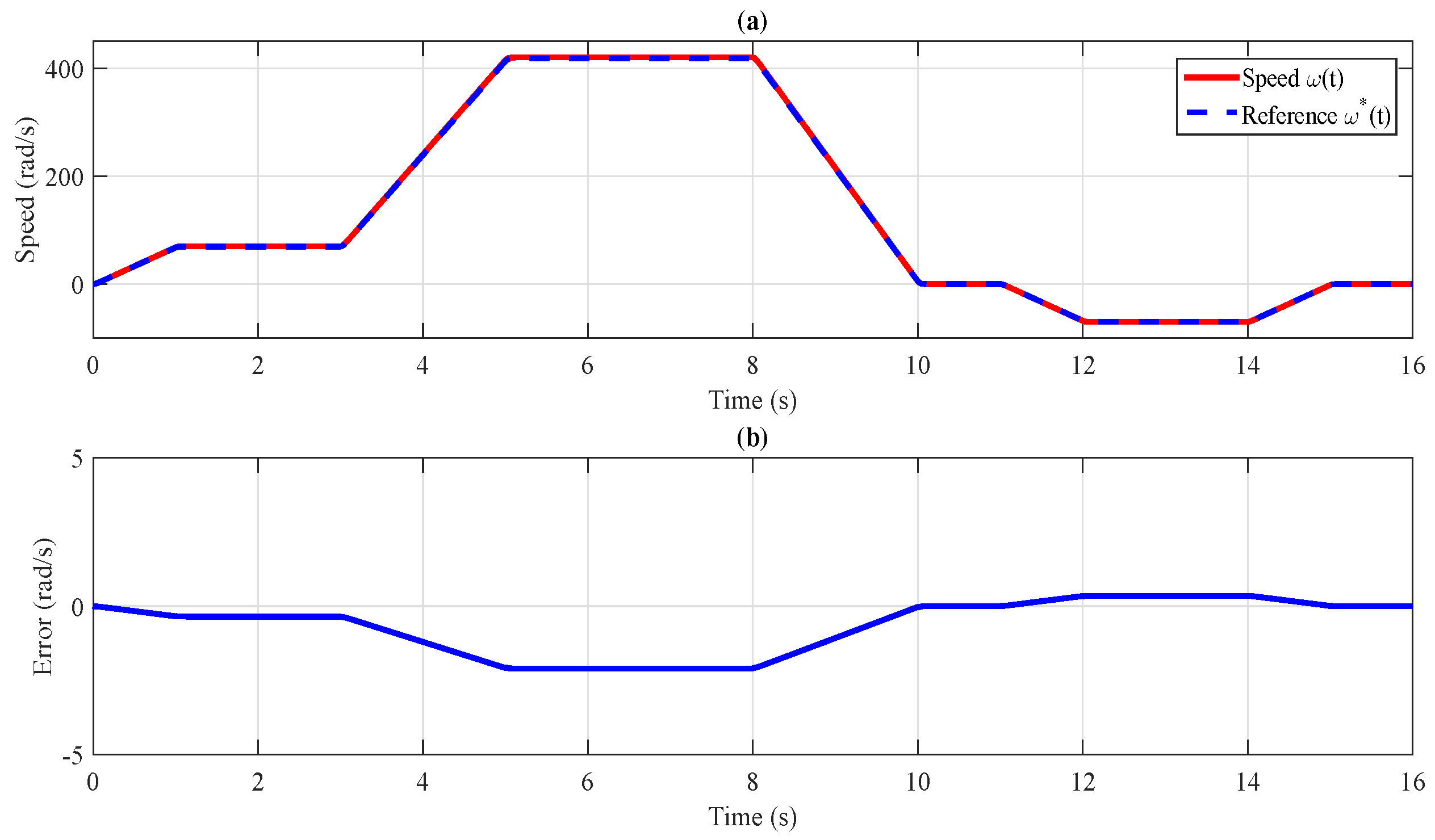
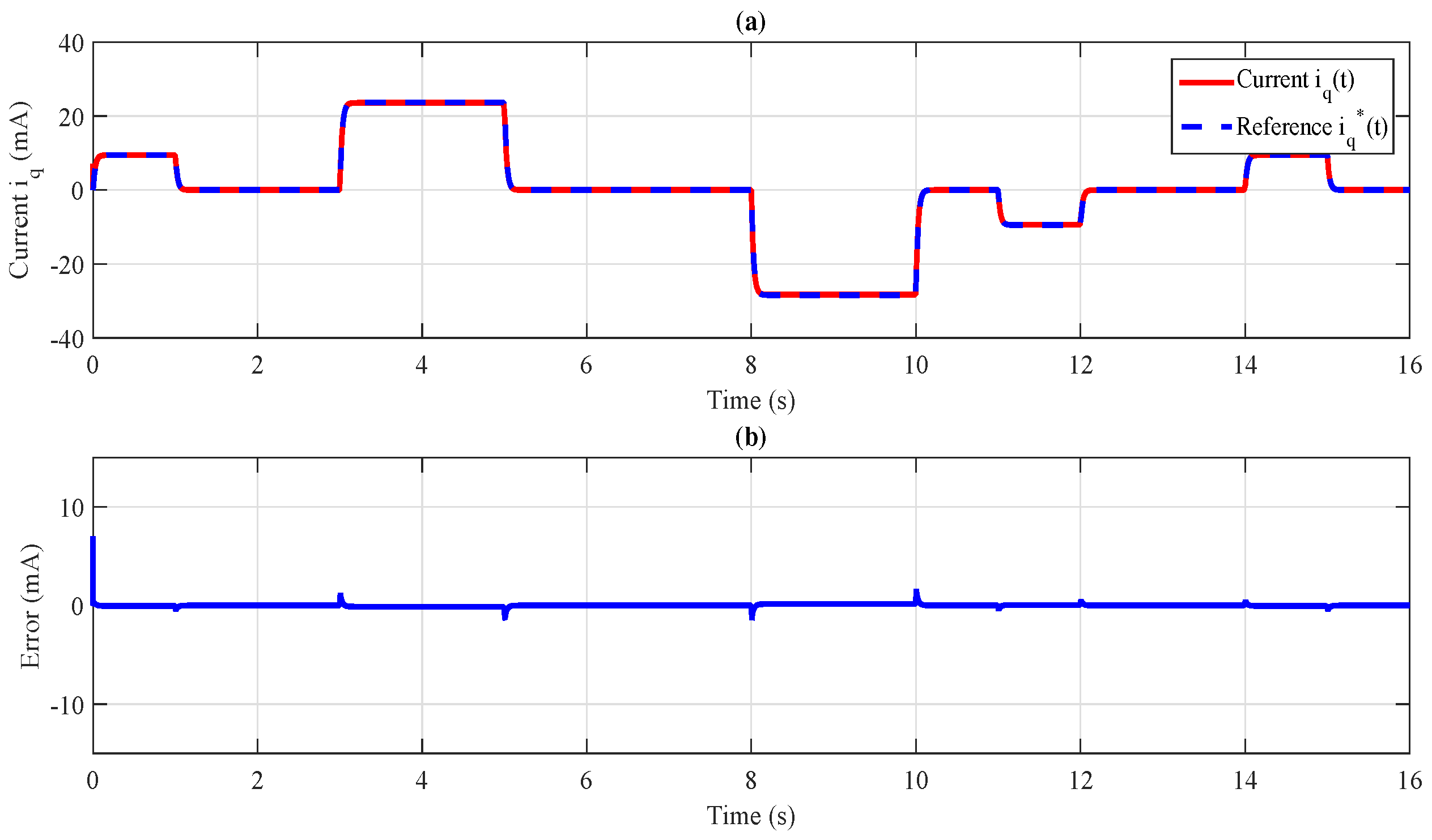
4.1. Simulation Results

The numerical evaluation was performed in MATLAB/SIMULINK using the Runge-Kutta method and a fixed step time of 50 $\mu$s with $K_d=150$ and $K_c=150$. This section presents the tracking speed, position, and torque trajectories. The tracking of torque was performed with a load.

4.1.1. Speed Trajectory Tracking

For the first evaluation, we consider speed trajectory tracking. In Figure 3a, the speed tracking is shown, and the desired trajectory is traced with a dotted line while the solid line corresponds to the angular speed of the rotor. The tracking error is presented in Figure 3b.

The trajectory tracking of the currents $i_d$ and $i_q$ are presented in Figure 4 and Figure 5.

According to [27], the technique used to obtain the temporal derivative has a natural phase lag due to the presence of low-pass filters in its structure, which generates an error in the speed tracking. As observed, the error increases with time due to the difference between the reference and the answer of the PMSM. Despite this, when the motor reaches the nominal speed, the tracking error is less than 1% of the reference maximum value.

4.1.2. Position Trajectory Tracking

For the second test, we consider the position tracking case with the profile given in Figure 6 as a reference trajectory. Figure 6a shows the position tracking performance; the desired trajectory is in the dotted line, while in the solid line is the angular position of the rotor of the PMSM. The tracking error is presented in Figure 6b. Trajectory tracking of the currents $i_d$ and $i_q$ are shown in Figure 7 and Figure 8. The position tracking error does not exceed 0.5% of the reference maximum value.

4.1.3. Torque Trajectory Tracking

Finally, we investigated the controller’s performance in the case of torque trajectory tracking. Load torque is applied at 3 s for 1 s. Then, at 6 s, a load torque is applied with the same magnitude but in the opposite sense for 1 s. In Figure 9a, the torque tracking is shown; the reference is in a dotted line, while in a solid line, the torque generated by the PMSM. Also, the tracking error is presented in Figure 9b. The torque tracking is maintained, and the error is less than 0.5 of the reference maximum value%.

To verify the trajectory tracking of the currents $i_d$ and $i_q$, the results in this case are presented in Figure 10 and Figure 11.

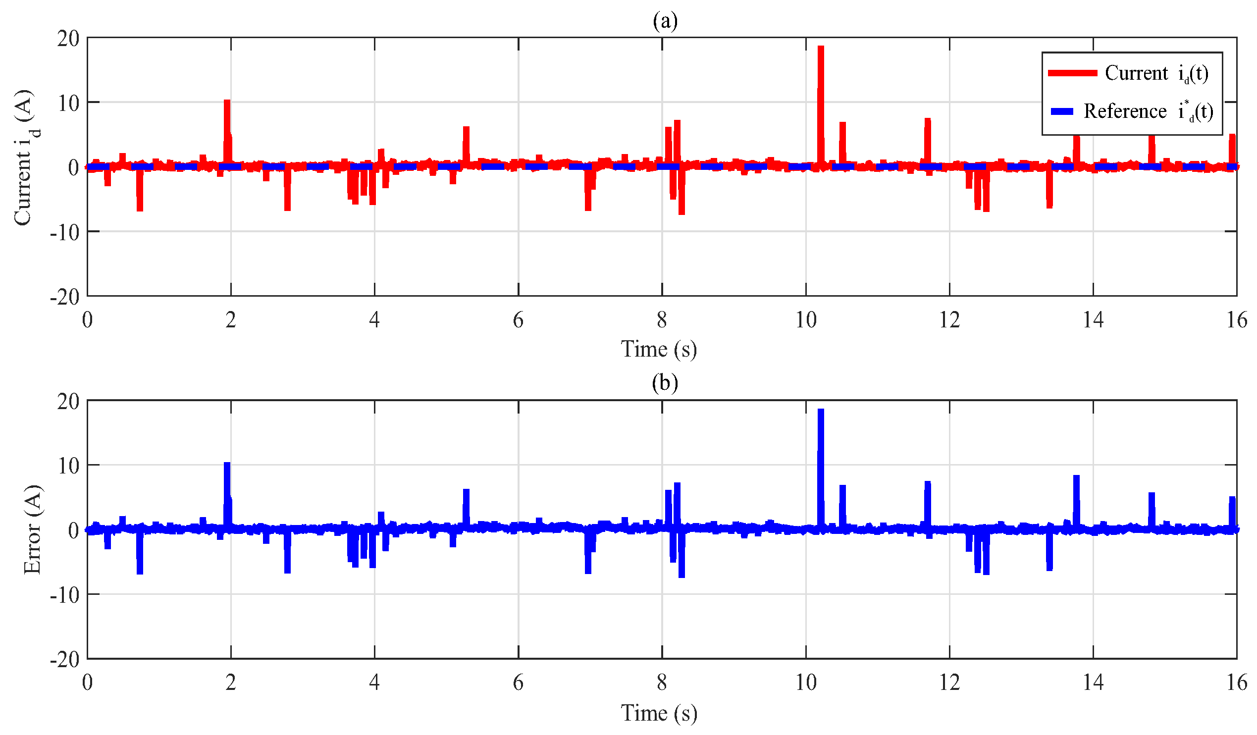
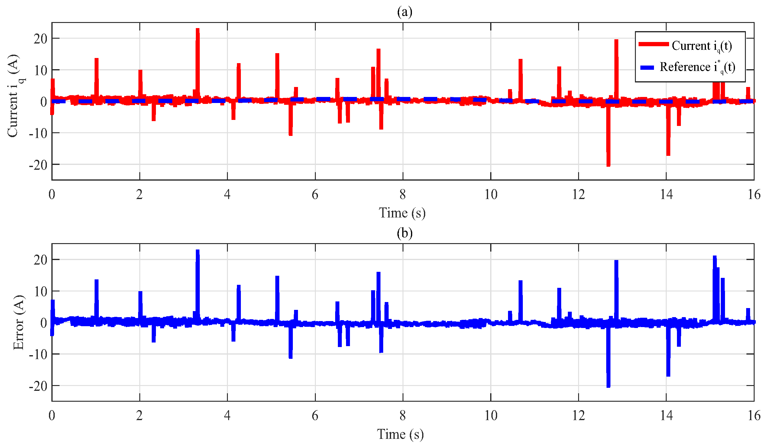
4.2. Experimental Results

The experimental evaluation was performed considering the PMSM parameters in Table 1. For simplicity, only the case of angular velocity was considered. A PMSM BLY172D-24 V-4000 (Anaheim Automation, Anaheim, CA, USA) integrated the test set-up with a nominal speed of 4000 rpm, an optical encoder as a position sensor, an inverter with a switching frequency of 20 kHz, and a 24 V DC-link voltage, two analog to digital converters, two current sensors, and a system of acquisition and processing based on an FPGA Virtex-5.

For the experimental test, the profile in Figure 12 is used as a reference trajectory for the angular speed. In Figure 12a, the speed tracking is shown; the desired trajectory is in a dotted line, and the speed of the rotor is traced in a solid line. The tracking error is presented in Figure 12b. In this case, the response exhibits oscillations that reach their greatest value when the PMSM operates at the lowest speed. When the motor reaches the nominal speed, the oscillations decrease until a value of 5 rad/s. However, tracking is achieved despite the effects of noise present in the measurements. The trajectory tracking of the currents $i_d$ and $i_q$ is shown in Figure 13 and Figure 14.

Note that, in contrast to the simulation results, the experimental behavior exhibits jitter overimposing the desired motor behavior. This is expected since for the real implementation, the controller must operate under the effect of the encoder, the switching of the power electronics involved in the inverter structure, and the digital implementation on the FPGA. Actually, this scenario imposes several sources of uncertainty that must be compensated by the control scheme. Hence, the obtained results state another evidence of the robustness properties of the proposed scheme.

5. Conclusions

The trajectory tracking control problem for the PMSM has been solved in this paper with the controller designed based on IDA-PBC. It is highlighted that the control law for speed tracking implies the control of position and torque. One disadvantage of this controller is that it is necessary to compute the first and second derivatives of the reference to generate the remaining trajectories. However, it is possible to obtain them efficiently using numerical estimation. In this case, the third-order numerical differentiator is used. Ongoing work addresses the controller implementation in the case of position and torque in experimental set-up to validate the numerical results.

References

1. Bose, B. Modern Power Electronics and AC Drives, Eastern Economy Ed.; Prentice Hall PTR: Hoboken, NJ, USA, 2002. [Google Scholar]
2. Naouar, M.W.; Naassani, A.; Monmasson, E.; Slama-Belkhodja, I. FPGA-Based Speed Control of Synchronous Machine using a P-PI Controller. In Proceedings of the 2006 IEEE International Symposium on Industrial Electronics, Montreal, QC, Canada, 9–13 July 2006; Volume 2, pp. 1527–1532. [Google Scholar] [CrossRef]
3. Li, W.; Lin, W.; Liu, P.X. Speed Tracking Control Based on Backstepping of Permanent Magnet Synchronous Motor with Uncertainty. In Proceedings of the 2007 International Conference on Mechatronics and Automation, Harbin, China, 5–8 August 2007; pp. 3657–3661. [Google Scholar] [CrossRef]
4. Solsona, J.; Valla, M.I.; Muravchik, C. Nonlinear control of a permanent magnet synchronous motor with disturbance torque estimation. IEEE Trans. Energy Convers. 2000, 15, 163–168. [Google Scholar] [CrossRef] [PubMed]
5. Rasmussen, H.; Vadstrup, P.; Borsting, H. Sensorless field oriented control of a PM motor including zero speed. In Proceedings of the IEEE International Electric Machines and Drives Conference, 2003. IEMDC’03, Madison, WI, USA, 1–4 June 2003; Volume 2, pp. 1224–1228. [Google Scholar] [CrossRef]
6. Wang, Y.; Zhu, J.G.; Guo, Y.G. A survey of direct torque control schemes for permanent magnet synchronous motor drives. In Proceedings of the 2007 Australasian Universities Power Engineering Conference, Perth, WA, Australia, 9–12 December 2007; pp. 1–5. [Google Scholar] [CrossRef]
7. Khanchoul, M.; Hilairet, M.; Normand-Cyrot, D. A passivity-based controller under low sampling for speed control of PMSM. Control Eng. Pract. 2014, 26, 20–27. [Google Scholar] [CrossRef]
8. Peng, J.; Yao, M. Overview of predictive control technology for permanent magnet synchronous motor systems. Appl. Sci. 2023, 13, 6255. [Google Scholar] [CrossRef]
9. Zhang, Q.; Zhang, C. Speed Control of PMSM Based on Fuzzy Active Disturbance Rejection Control under Small Disturbances. Appl. Sci. 2023, 13, 10775. [Google Scholar] [CrossRef]
10. Chen, L.; Zhang, H.; Wang, H.; Shao, K.; Wang, G.; Yazdani, A. Continuous adaptive fast terminal sliding mode-based speed regulation control of pmsm drive via improved super-twisting observer. IEEE Trans. Ind. Electron. 2023, 71, 5105–5115. [Google Scholar] [CrossRef]
11. Belkhier, Y.; Achour, A.; Bures, M.; Ullah, N.; Bajaj, M.; Zawbaa, H.M.; Kamel, S. Interconnection and damping assignment passivity-based non-linear observer control for efficiency maximization of permanent magnet synchronous motor. Energy Rep. 2022, 8, 1350–1361. [Google Scholar] [CrossRef]
12. Belkhier, Y.; Shaw, R.N.; Bures, M.; Islam, M.R.; Bajaj, M.; Albalawi, F.; Alqurashi, A.; Ghoneim, S.S. Robust interconnection and damping assignment energy-based control for a permanent magnet synchronous motor using high order sliding mode approach and nonlinear observer. Energy Rep. 2022, 8, 1731–1740. [Google Scholar] [CrossRef]
13. Ortega, R.; Spong, M.W. Adaptive motion control of rigid robots: A tutorial. In Proceedings of the 27th IEEE Conference on Decision and Control, Austin, TX, USA, 7–9 December 1988; Volume 2, pp. 1575–1584. [Google Scholar] [CrossRef]
14. Ortega, R.; Liu, Z.; Su, H. Control via interconnection and damping assignment of linear time-invariant systems: A tutorial. Int. J. Control 2012, 85, 603–611. [Google Scholar] [CrossRef]
15. Ortega, R.; van der Schaft, A.; Maschke, B.; Escobar, G. Interconnection and damping assignment passivity-based control of port-controlled Hamiltonian systems. Automatica 2002, 38, 585–596. [Google Scholar] [CrossRef]
16. Gomez-Estern, F.; der Schaft, A.V. Physical Damping in IDA-PBC Controlled Underactuated Mechanical Systems. Eur. J. Control 2004, 10, 451–468. [Google Scholar] [CrossRef]
17. Chang, D.E. Generalization of the IDA-PBC method for stabilization of mechanical systems. In Proceedings of the 18th Mediterranean Conference on Control and Automation, MED’10, Marrakech, Morocco, 23–25 June 2010; pp. 226–230. [Google Scholar]
18. Rodriguez, H.; Ortega, R.; Escobar, G. A robustly stable output feedback saturated controller for the Boost DC-to-DC converter. In Proceedings of the 38th IEEE Conference on Decision and Control (Cat. No.99CH36304), Phoenix, AZ, USA, 7–10 December 1999; Volume 3, pp. 2100–2105. [Google Scholar]
19. Galaz, M.; Ortega, R.; Bazanella, A.S.; Stankovic, A.M. An energy-shaping approach to the design of excitation control of synchronous generators. Automatica 2003, 39, 111–119. [Google Scholar] [CrossRef]
20. Batlle, C.; Doria-Cerezo, A.; Ortega, R. Power flow control of a doubly-fed induction machine coupled to a flywheel. In Proceedings of the 2004 IEEE International Conference on Control Applications, Taipei, Taiwan, 2–4 September 2004; Volume 2, pp. 1645–1650. [Google Scholar]
21. Petrovic, V.; Ortega, R.; Stankovic, A.M. Interconnection and damping assignment approach to control of PM synchronous motors. IEEE Trans. Control Syst. Technol. 2001, 9, 811–820. [Google Scholar] [CrossRef]
22. Ortega, R.; Garcia-Canseco, E. Interconnection and Damping Assignment Passivity-Based Control: A Survey. Eur. J. Control 2004, 10, 432–450. [Google Scholar] [CrossRef]
23. Fujimoto, K.; Sakurama, K.; Sugie, T. Trajectory tracking control of port-controlled Hamiltonian systems via generalized canonical transformations. Automatica 2003, 39, 2059–2069. [Google Scholar] [CrossRef]
24. Fujimoto, K.; Sugie, T. Canonical transformation and stabilization of generalized Hamiltonian systems. Syst. Control Lett. 2001, 42, 217–227. [Google Scholar] [CrossRef]
25. Borja-Rosales, P. Passivity-Based Control Using Coordinates Change. Master’s Thesis, Universidad Nacional Autonoma de Mexico, Mexico, 2013. (In Spanish). [Google Scholar]
26. Chiasson, J. Modeling and High Performance Control of Electric Machines; IEEE Press Series on Power Engineering; Wiley: Hoboken, NJ, USA, 2005. [Google Scholar]
27. Mujica, H.; Espinosa-Pérez, G. Nonlinear Passivity-Based Control of Induction Motors for High Dynamic Performance. Rev. Iberoam. Autom. Inform. Ind. 2014, 11, 32–43. [Google Scholar] [CrossRef]
Figure 1. (a) Control scheme for tracking speed trajectories. (b) Control scheme for tracking position trajectories. (c) Control scheme for tracking torque trajectories.
Applsci 14 07977 g001
Figure 2. Control scheme.
Applsci 14 07977 g002
Figure 3. (a) Speed ω ( t ) and reference. (b) Trajectory tracking error.
Applsci 14 07977 g003
Figure 4. (a) Current i d ( t ) and reference. (b) Trajectory tracking error.
Applsci 14 07977 g004
Figure 5. (a) Current i q ( t ) and reference. (b) Trajectory tracking error.
Applsci 14 07977 g005
Figure 6. (a) Position θ ( t ) and reference. (b) Trajectory tracking error.
Applsci 14 07977 g006
Figure 7. (a) Current i d ( t ) and reference. (b) Trajectory tracking error.
Applsci 14 07977 g007
Figure 8. (a) Current i q ( t ) and reference. (b) Trajectory tracking error.
Applsci 14 07977 g008
Figure 9. (a) Torque τ ( t ) and reference. (b) Trajectory tracking error.
Applsci 14 07977 g009
Figure 10. (a) Current i d ( t ) and reference. (b) Trajectory tracking error.
Applsci 14 07977 g010
Figure 11. (a) Current i q ( t ) and reference. (b) Trajectory tracking error.
Applsci 14 07977 g011
Figure 12. (a) Speed ω ( t ) and reference. (b) Trajectory tracking error.
Applsci 14 07977 g012
Figure 13. (a) Current i d ( t ) and reference. (b) Trajectory tracking error.
Applsci 14 07977 g013
Figure 14. (a) Current i q ( t ) and reference. (b) Trajectory tracking error.
Applsci 14 07977 g014