Article

Simulation Analysis and Experimental Investigation on the Fluid–Structure Interaction Vibration Characteristics of Aircraft Liquid-Filled Pipelines under the Superimposed Impact of External Random Vibration and Internal Pulsating Pressure

1
Administration and Support Department, National University of Defense Technology, Changsha 410073, China
2
College of Intelligence Science and Technology, National University of Defense Technology, Changsha 410073, China
*
Author to whom correspondence should be addressed.
Appl. Sci. 2024, 14(17), 8008; https://doi.org/10.3390/app14178008 (registering DOI)
Submission received: 3 August 2024 / Revised: 2 September 2024 / Accepted: 2 September 2024 / Published: 7 September 2024

Abstract

:
This paper investigated the fluid–structure interaction vibration response of an aircraft liquid-filled pipeline under external random vibration and internal pulsating pressure. First, the fluid–structure interaction solution is theoretically analyzed, and the advantages and disadvantages of the direct coupling method and the separation coupling method are compared, with the latter chosen as the simulation analysis method in this study. Second, taking the U-shaped oil pipeline of an aircraft engine as an example, simulation modeling was performed to compare and analyze the fluid–structure interaction vibration response of aircraft liquid-filled pipelines under different working conditions, obtaining the vibration response characteristics of stress danger points under various conditions. Finally, a test bench for an aircraft liquid-filling pipeline was built to explore the influence of external random vibrations with different kurtoses, different pipe wall thicknesses and different working conditions on the vibration response danger points of aircraft liquid-filling pipelines, verifying the simulation conclusions and providing a basis for aircraft liquid-filling pipeline design.

1. Introduction

Fluid-filled pipelines are extensively employed in industrial apparatuses such as those in the energy, power, petroleum and chemical sectors, as well as diverse equipment like aerospace aircraft, ships, submarines and land vehicles. Taking the aircraft pipeline system as an illustration, the vibration issue has consistently been the key concern for aircraft designers and reliability assessors. On the one hand, when the aircraft is soaring at high altitudes and influenced by turbulence, the vibrations generated by the aircraft are transmitted through the fuselage to the pipes. On the other hand, due to the pulsation of the aircraft’s plunger pump during its operation, the fluid within the pipe is frequently in a state of pressure pulsation. These two types of vibrations, through mutual coupling, form the highly significant and complex fluid–structure interaction effect, which poses a severe safety hazard to aircraft flights.
Many scholars have performed studies on this aspect. Lian et al. [1] established a one-dimensional (1D) numerical model for the fluid–solid interaction (FSI) behavior of a pipe and evaluated the vibration magnitude of both solids and fluids in the headrace tunnel of a pumped storage power station. Liu et al. [2] established a fluid–structure interaction vibration model of the aviation hydraulic pipeline system and verified the validity and accuracy of the vibration model via the finite element method. Zhang and Cui [3] investigated the fluid flow-induced vibrations in a pipeline system based on Housner’s differential vibration equation of fluid pipelines, and obtained the corresponding equations for the natural frequencies and dynamic response of the system by simplifying the derivation of the inherent characteristics and dynamic behavior of a hydraulic pipeline system. Zhang et al. [4] simulated the flow around thermowells through two-way thermal fluid–structure interactions by using the LES method and proposed measures for improving the thermowell safety in petroleum cracking gas pipeline systems. Su and Gong [5] analyzed vibration characteristics of pipelines under various external excitations by using the fluid–structure interaction method. In their study, a three-dimensional high-pressure pipeline model composed of corrugated pipes, multi-section bent pipes and other auxiliary structures was established. They used a two-way fluid–solid coupling method to examine the vibration characteristics of a kerosene pipeline at the outlet of the first-stage pump of a liquid oxygen kerosene engine; we have added the related description in the article. Liang et al. [6] analyzed the dynamic characteristics and dynamic response of the elbow with simultaneous dual-thread analysis method. The abnormal vibration of natural gas station pipelines seriously threatens the safety of pipeline transportation, and so Liu et al. [7] carried out the vibration analysis of a station yard pipeline by taking the outbound pipeline of the Yongchang pressure station as their research object. Qu et al. [8] simplified the support as an equivalent and a spring and investigated dynamic characteristics of a pipeline under different support stiffness conditions by using the bidirectional fluid–structure interaction analysis method. Beatty and Elías-Zúñiga [9] investigated the Mullins effect in the small amplitude transverse vibration of a stretched rubber membrane and graphically illustrated the analytical relations for two kinds of non-Gaussian molecular network models for rubber elasticity. Jiang et al. [10] proposed a novel fatigue life prediction model for electronic components under non-Gaussian random vibration excitations based on random vibration and fatigue theory. Wang and Song [11] proposed the Gaussian mixture-based equivalent linearization method (GM-ELM) which can decompose the non-Gaussian response of a nonlinear system into multiple Gaussian responses of linear single-degree-of-freedom oscillators. Zheng et al. [12] presented a new control method for multi-input, multi-output, stationary, non-Gaussian random vibration tests using time domain randomization, and analyzed the generation process of stationary and coupled reference non-Gaussian signals by specified reference skewness, kurtoses and spectra. Ren et al. [13] studied the generation and closed-loop control of multi-shaker, non-stationary, non-Gaussian random vibration signals with the modified time domain randomization technique and theoretically derived the kurtosis relationship between the one frame pseudo-random signal and consecutive true random signal.
Domestic and foreign scholars mostly consider the vibration response of liquid-filled pipelines only under the action of an external random vibration load, and few studies have been conducted on the fluid–structure interaction vibration response characteristics of liquid-filled pipelines under the action of existing external random vibration load and internal fluid pulsating pressure. The pipeline of a hydraulic system is constantly subjected to two kinds of loads: complex external random vibration and internal fluid pulsation pressure. The problem of the complex fluid–structure interaction vibration response needs to be studied and solved, especially when the external load belongs to non-Gaussian vibration, as the problem cannot be solved by traditional Gaussian vibration analysis methods (such as the power spectral density method). Different from previous studies, this paper studied the fluid–structure interaction vibration response of an aircraft liquid-filled pipeline under an external random vibration load and internal pulsating pressure, and explored the influence of external random vibration with different kurtoses, different pipe wall thicknesses and different working conditions on the vibration response danger points of aircraft liquid-filled pipelines. We believe that the research result has great practical significance for optimizing the design of aircraft oil pipelines.

2. Theoretical Foundation

Fluid–structure interaction (FSI) is a branch of engineering at the interface of fluid mechanics and solid mechanics. It is a discipline that studies the interaction and mutual influence between fluids and solids. It is currently widely used in ocean engineering, aerospace engineering, shipbuilding and other engineering fields. The calculation of fluid–structure interactions can be regarded as the simultaneous calculation of fluids and solids, neither of which can be ignored, because the characteristics of fluids and solids are considered at the same time. Compared with the calculation of fluids and solids separately, fluid–structure interactions can improve the calculation efficiency and save the calculation cost, and at the same time, the results can be closer to the actual project.

2.1. Analysis Method

The solution models of fluid–structure interaction theory mainly include 4-equation, 8-equation, 12-equation and 14-equation models, among which 4-equation and 8-equation models are mainly used to solve simple straight pipe and curved pipe calculations. At present, the 4-equation model and 8-equation model are widely used in practical applications. Nowadays, the theoretical calculation method of fluid–structure interactions has been fully verified in the project, which has the advantages of clear mathematical equations, small calculation amount and high calculation efficiency. However, for complex models and boundary conditions in the project, the theoretical calculation method inevitably ignores some details. Also, the theoretical calculation method will be less efficient in establishing a model equivalent to the actual project.
Based on the corresponding theoretical calculation model, the finite element method, which discretizes the model, has become the mainstream calculation method of fluid–structure interactions. In the finite element method of fluid–structure interaction calculation, the governing equation is the core part, which mainly consists of a fluid governing equation, structure governing equation and fluid–structure interaction governing equation.

2.2. Fluid Governing Equation

The fluid flow process follows the three basic physical conservation laws of mass, energy and momentum. When the fluid is mixed with other components, it also follows the conservation law of the components. Generally, compressible fluids can be described by the following governing equations:
Mass conservation equation:
ρ f t + ( ρ f v ) = 0
Momentum conservation equation:
ρ f v t + ( ρ f v v τ f ) = f f
where, t represents time, f f represents volume force vector, ρ f represents the density of the fluid, v represents the velocity vector of the fluid and τ f represents the shear force tensor, which can be expressed as:
τ f = ( p + μ v ) I + 2 μ e
where, p represents the pressure of the fluid, μ represents the dynamic viscosity and e represents the velocity stress tensor of the fluid, e = 1 2 ( v + v T ) .
If the energy equation is considered, the energy equation in the form of total enthalpy can be described as:
( ρ h t o t ) t p t + ( ρ f v h t o t ) = ( λ T ) + ( v τ ) + v ρ f f + S E
where, λ represents the heat absorption coefficient, h t o t represents the total enthalpy and S E represents the energy source term.

2.3. Solid Governing Equation

The governing equation of the solid structure part is mainly based on Newton’s second law:
ρ s d ¨ s = σ s + f s
where, ρ s represents the density of a solid, f s represents the volume force vector, d ¨ s represents the acceleration vector and σ s represents the Cauchy stress tensor, which can be expressed as:
σ s = C ε s
where, C represents elasticity tensor and εs represents Cauchy strain tensor.

2.4. Fluid–Structure Interaction Governing Equation

Similarly, fluid–structure interactions should also follow the basic physical conservation laws, and the variables such as stress ( τ ), temperature ( T ), displacement ( d ) and heat flow ( q ) between the two phases of the fluid domain and the solid domain should be conserved or equal at the fluid–structure interaction interface, so that the following equations are satisfied:
{ τ f n f = τ s n s T f = T s d f = d s q f = q s
where, the subscript f represents the fluid and the subscript S represents the solid.

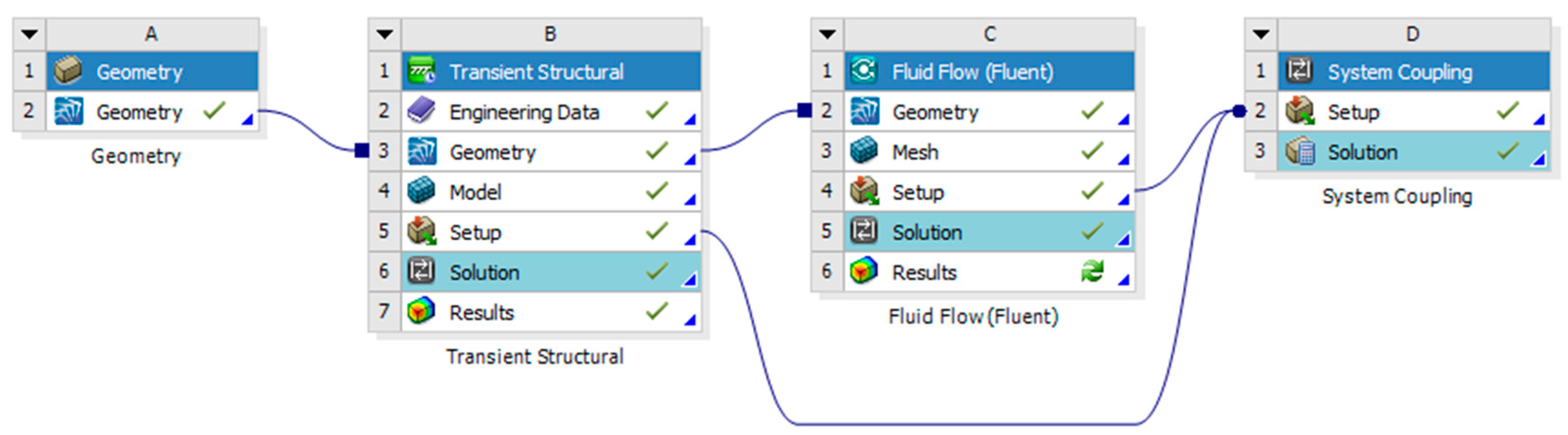
2.5. Fluid–Structure Interaction Solution Method

According to the above governing equations, the fluid–structure interaction problem can be solved by giving appropriate initial conditions, boundary conditions and solution parameters. Fluid–structure interaction solution methods are generally divided into the direct coupling method and the separate coupling method. The direct coupling method solves fluid and solid control equations by integrating them into the same matrix equation, that is, the fluid and solid equations are solved simultaneously in the same solver.
[ A f f A f s A s f A s s ] [ Δ X f k Δ X s k ] = [ B f B s ]
where, k represents the number of iterations, A f f represents the fluid control matrix, Δ X f k represents the flow field to be solved, B f represents the external force of fluid, A s s represents the solid control matrix, Δ X s k represents the solid region parameters to be solved, B s represents the solid external force and both A s f and A f s represent the fluid–structure interaction matrix.
The direct coupling method has the characteristics of no time lag, and its solving precision is very high. However, for the current computational fluid dynamics (CFD ANSYS Fluent 22) and computational solid mechanics (CSM Mechanical APDL 22) simulation software, its fluid and solid solvers often cannot be carried out at the same time, and it is difficult to directly couple fluid and solid solutions. It is very difficult to solve convergence at the same time. So, the direct coupling method can only be applied to very simple structure models, and has not played a practical role in industry. The separate coupling method separates and solves the fluid governing equation and solid governing equation by putting them in the CFD and CSM calculation modules respectively, and exchanging data through the fluid–solid interface. When the CFD calculation reaches convergence, the results will be transferred to CSM calculation modules for the solid solution, and the results will be transferred to CFD calculation modules for fluid calculation at the next moment after the solid solution converges. Such a data transfer calculation greatly improves the calculation efficiency, and the CFD software and CSM software do not need to make great changes to achieve fluid–structure interaction solutions, which can realize large-scale fluid–structure interaction solutions in practical projects. Almost all commercial ANSYS Workbench 2022 R1 software adopts the separation coupling method, and this simulation method is also used in this paper.

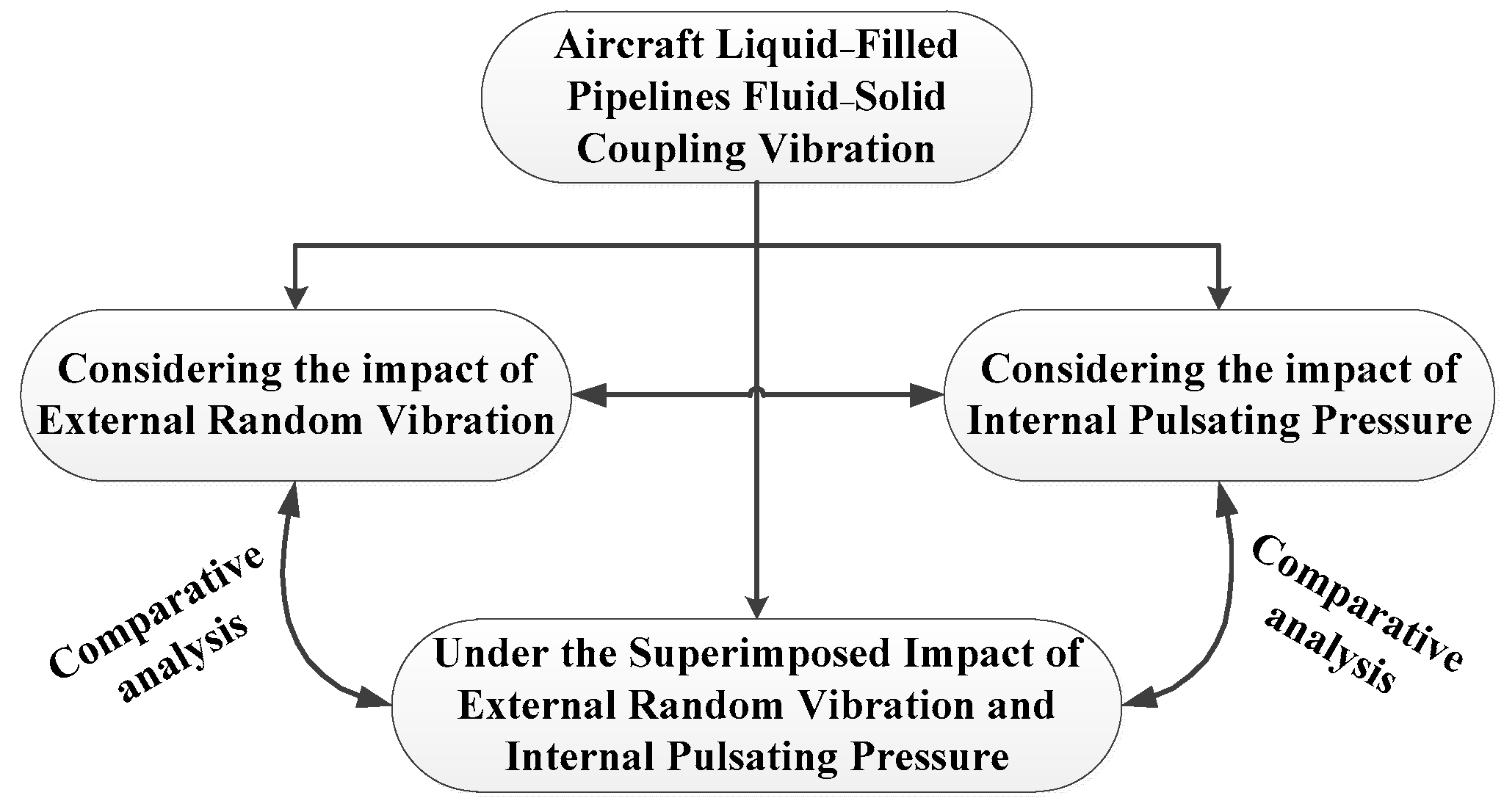
3. Research Strategy

The load on liquid-filled pipelines can be divided into two categories. One is the random vibration of the external environment and the other is the periodic load generated in the inner wall of the pipeline due to the pulsation of the fluid pressure inside the pipeline. Under the combined action of these two types of loads, complex fluid–structure interaction vibrations occur in liquid-filled pipelines. In order to explore the vibration response of the pipeline under two types of loads more comprehensively, the vibration response of the pipeline under external random excitation and the vibration response of the pipeline under internal fluid pressure pulsation are studied separately. Finally, the fluid–structure interaction vibration response of liquid-filled pipelines under external random excitation and internal fluid pressure pulsation are studied by the two types of loads. The research idea of the fluid–structure interaction vibration response analysis of liquid-filled pipelines is shown in Figure 1.

4. Simulation Analysis of Aircraft Liquid-Filled Pipelines
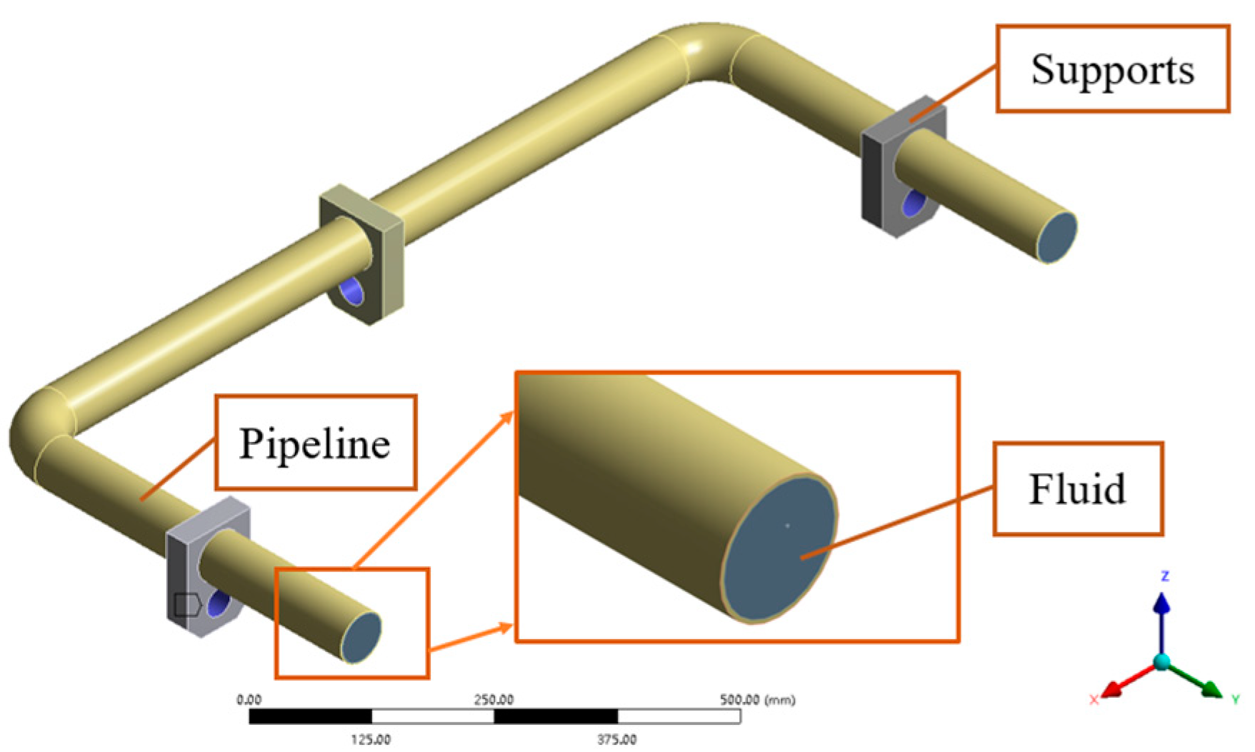
4.1. Physical Model

Aircraft engine oil pipelines are all curved and have complex layouts. Figure 2 shows the physical drawings of the pipeline layout of the Russian Su-35 aircraft 117C engine. It can be seen from the figure that these pipes are mainly curved, with most of the elbow angles reaching 90 degrees. Due to the movement of fluid in the pipe, excessive stress often occurs at the corner of the pipe. At the same time, there are often some supports in the straight pipe section to attach the pipe to the engine or fuselage. In the aircraft, these connections transmit vibrations from the engine, as well as vibrations from unstable airflow during the operation of the aircraft, exacerbating the vibration of the pipe. Therefore, in this paper, a typical U-shaped pipe with an angle of 90 degrees has been selected as the research object. The pipe is fixed by a support, and then the support is fixed to the bottom plate connected to the vibration table. Figure 3 shows the physical diagram of the U-shaped pipeline tested in this paper, which was taken by the authors.

4.2. Finite Element Modeling

4.2.1. Model Establishment of Pipeline

A model of the liquid-filled pipeline is shown in Figure 4. The pipeline part and the fluid part of the liquid-filled pipeline were established by using Ansys Workbench. It is composed of three parts: pipe, fluid and support. The outer diameter of the U-shaped pipe is 60 mm, and the thickness of the pipe wall is 2 mm.

4.2.2. Grouping of Simulation Analysis

According to the above research proposals, the simulation analysis of the vibration response of a liquid-filled pipe is divided into three groups. Group A is an empty pipe, which is only stimulated by external random excitation. Group B is only affected by the pulsating fluid pressure in the pipe. Group C is subjected to the combined action of external random excitation and internal pulsating pressure (referred to as “combined action”). The results of the grouping are shown in Table 1.

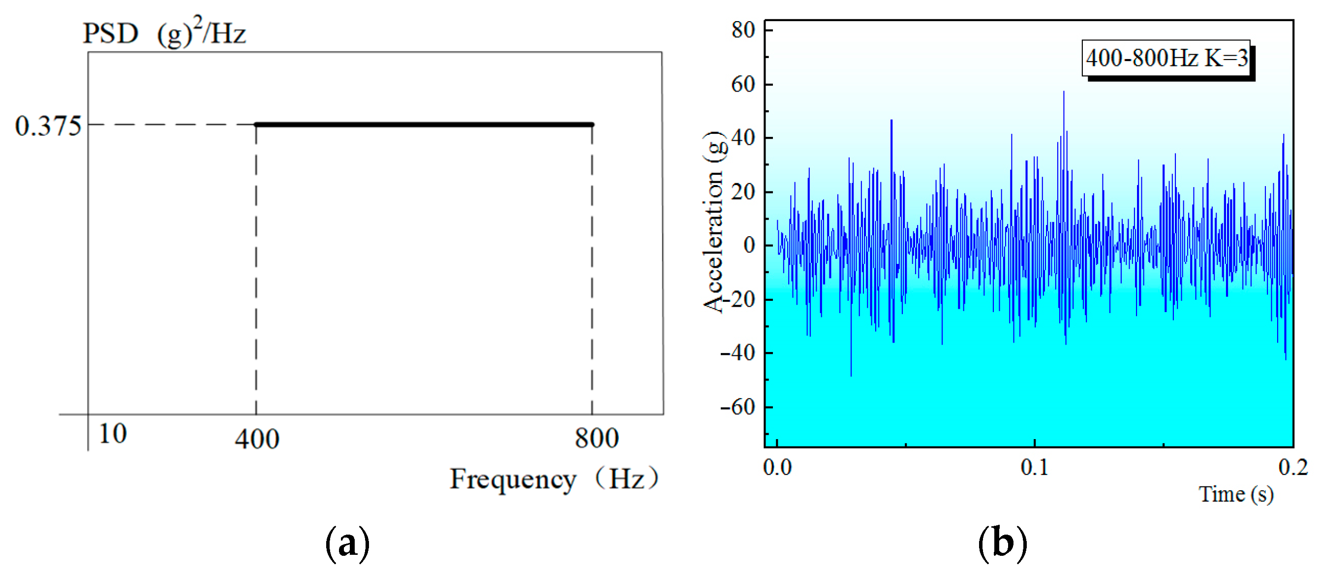
4.2.3. Load Generation

The type of load on a pipeline filled with liquid can be divided into two categories: an external random load and a pulsating pressure load inside the pipeline.

Random Load Extraction

Transient dynamics analysis requires time domain loads as input signals, and these time domain load data need to have different load parameters to control the relevant variables. In this paper, the random vibration signal measured directly from the vibration table is used as the external random load excitation of the pipeline. A 5-ton electromagnetic vibration test bench was selected, a non-Gaussian vibration controller developed by the laboratory (which can control the kurtosis of the signals, so as to obtain the Gaussian and non-Gaussian vibration signals) was adopted and the vibration signal test system of the B&K company was used to measure the acceleration of the vibration table, so as to obtain the time domain load data. Modal simulation was carried out under the two working conditions (empty pipeline and liquid-filled pipeline). The modal module in Ansys Workbench 2022 R1 software was used. The diameter of the U-shaped pipeline is 60 mm and the thickness of the pipe wall is 2 mm. The grid division method of the pipeline is the Sweep Method and the grid division method of the fluid is Tetrahedron. The number of grid nodes is 142,078 and the number of cells is 84,430. The modal simulation shows that the first two natural frequencies of the pipeline in the empty pipe state are 529.54 Hz and 532.27 Hz, respectively, and the first two natural frequencies of the pipeline when it is filled with liquid are about 430 Hz. In order to excite the first two modes of the pipeline to generate a sufficient vibration response, the frequency band of the extracted random vibration load is 400–800 Hz. The spectral type is a flat spectrum, the root mean square acceleration value is 15 g, the kurtosis value is 3 (considering the Gaussian distribution load first), the sampling frequency is 2560 Hz, the analytical spectral line is 200 and a random time domain signal with 1 frame of 0.2 s and 512 data points is extracted. Figure 5a shows the power spectral density function of the acceleration load, and Figure 5b shows the time domain signal of the acceleration load.

Generation of Fluid Pulsation Pressure in Pipe

The fluid pressure pulsation in the pipe is due to changes in equipment working conditions, such as the sudden opening and closing of the valve, which will form a water hammer effect in an instant. The water hammer will cause a continuous oscillation of the pressure in the pipe, forming a periodic high and low pressure. For example, the reciprocating movement of the plunger pump in the aircraft engine will cause the oil pressure in the pipe to change periodically. Generally speaking, the pressure change curve over time is a square wave, and the high pressure duration of the square wave is basically the same as the low pressure duration. At the same time, the period of the liquid pulsating pressure in the plunger pump is not very high, generally not more than 20 Hz. Therefore, the pulsating pressure square wave is used to simulate the pulsating pressure of the fluid in the simulation. Figure 6 shows the time domain load of the pulsating pressure signal. The pressure amplitude is 5 MPa, the pressure pulsation frequency is 20 Hz and the pulsation waveform is a square wave.

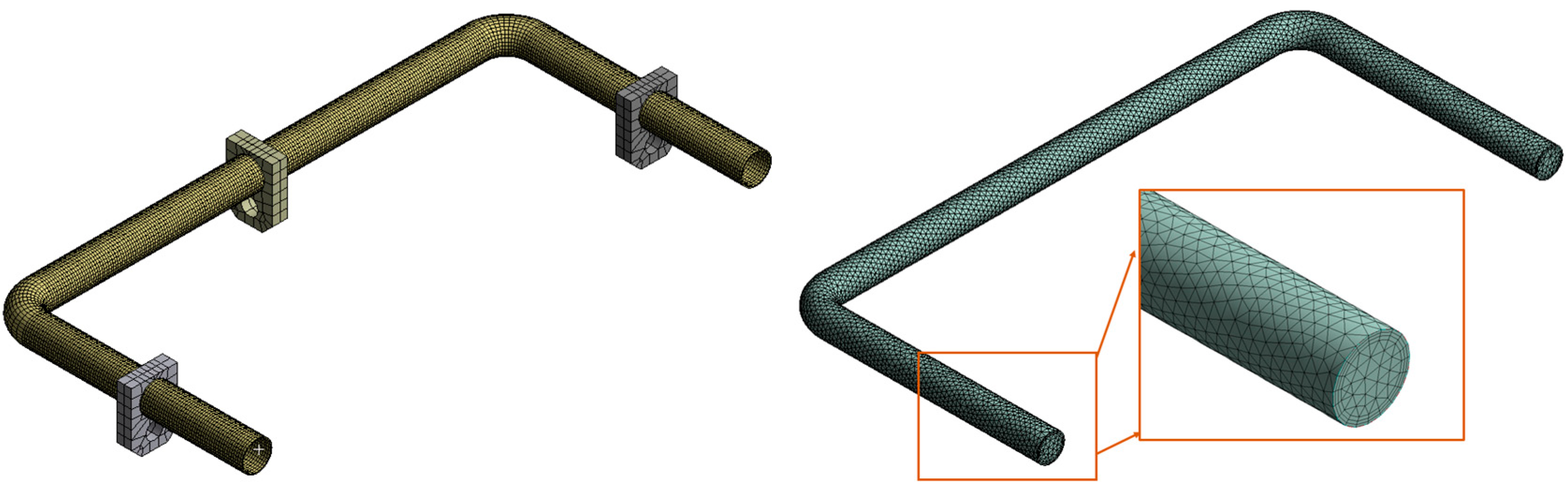
4.3. Mesh Generation

The pipeline, fluid and support are gridded. The pipeline mesh generation method is Sweep and the fluid mesh generation method is Tetrahedron. The fluid mesh is also controlled by inflation and the mesh volume is controlled to 10 mm. Free mesh (Automatic) is used for the rest of the support. The meshing of the pipe and fluid parts is shown in Figure 7.

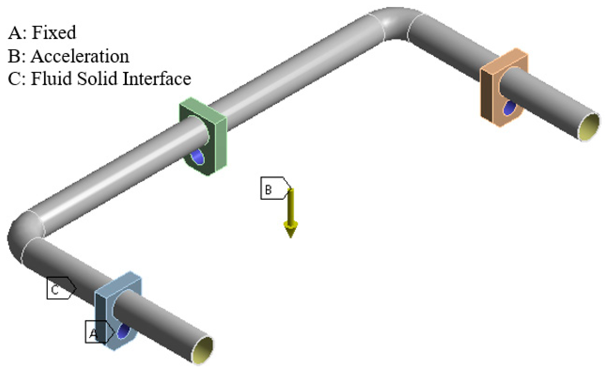
4.4. Boundary Conditions and Parameters Setting

This paper adopts the two-way fluid–structure interaction calculation method based on Ansys Workbench, and the modules used mainly include the transient structural module, fluent module and system coupling module. The data transfer mode is shown in Figure 8. Relevant settings are carried out in the solid module (transient dynamics module) and fluid module (fluent module) respectively, and then the settings are transferred to the system coupling module for the coupling calculation. For Group A ATC simulation, only random vibration analysis of the ATC is performed. Group A simulation does not require the fluent and system coupling modules to be involved in the calculation.
As shown in Figure 9, the superstructure input method was used to apply the foundation excitation, suppress the fluid part, set the fluid–structure interaction surface, fix the three supports and apply the acceleration load in the Z direction, as shown in Figure 5b. The calculation time was specified as 0.2 s and the load component as 512.
The U-shaped tube is made of 304 stainless steel, the support material is made of structural steel and the fluid part is no. 32 hydraulic oil. The relevant parameters of the materials are shown in Table 2, which is derived from the engineering material data library of the Ansys Workbench simulation software.

4.5. Simulation Results and Comparative Analysis

Under the above simulation conditions and simulation groups, the vibration response danger points of each simulation result were analyzed and the relevant stress values at the danger points were extracted. The stress was counted by rain flow, and the simulation results of each group were analyzed and compared.

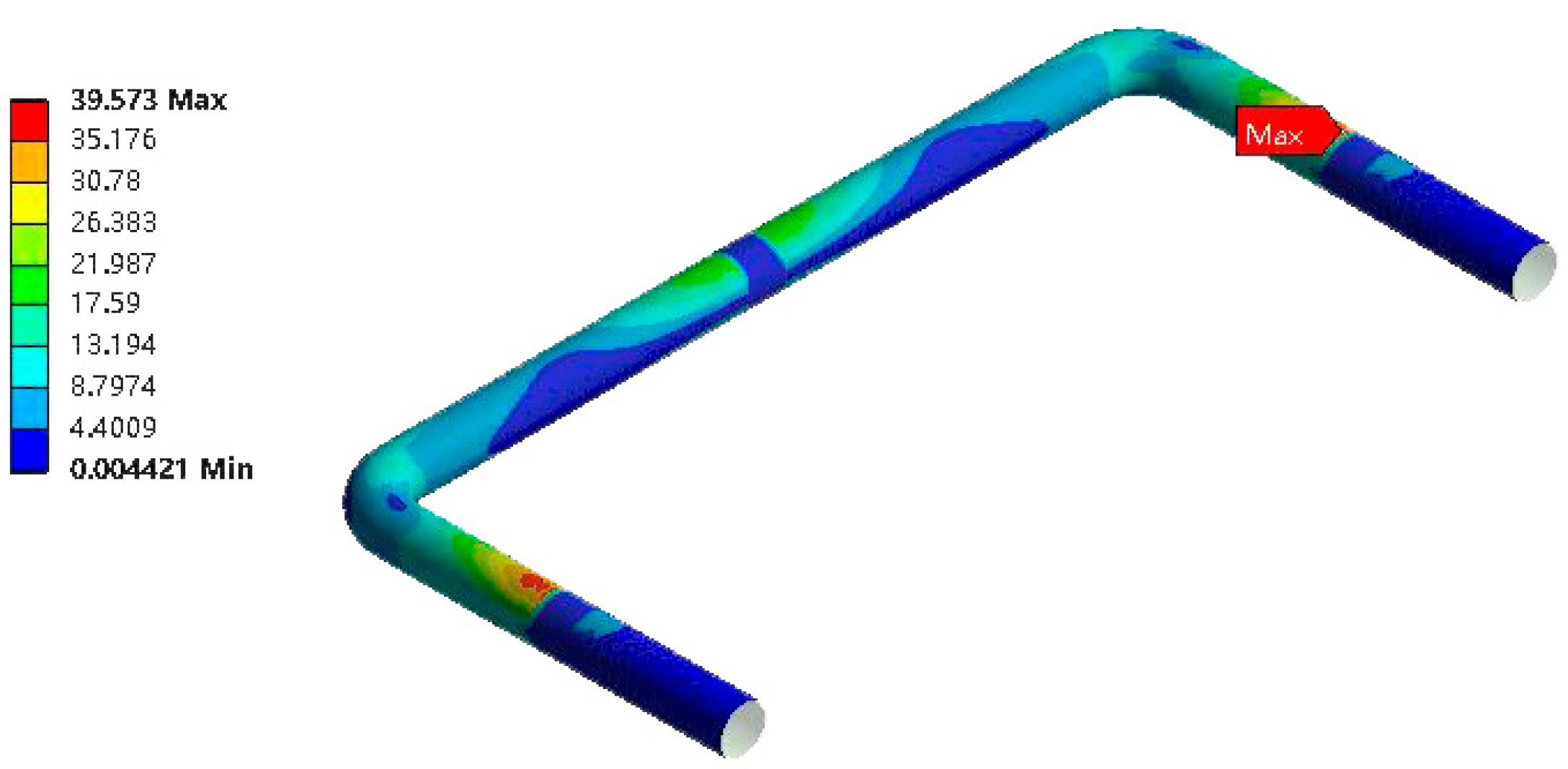
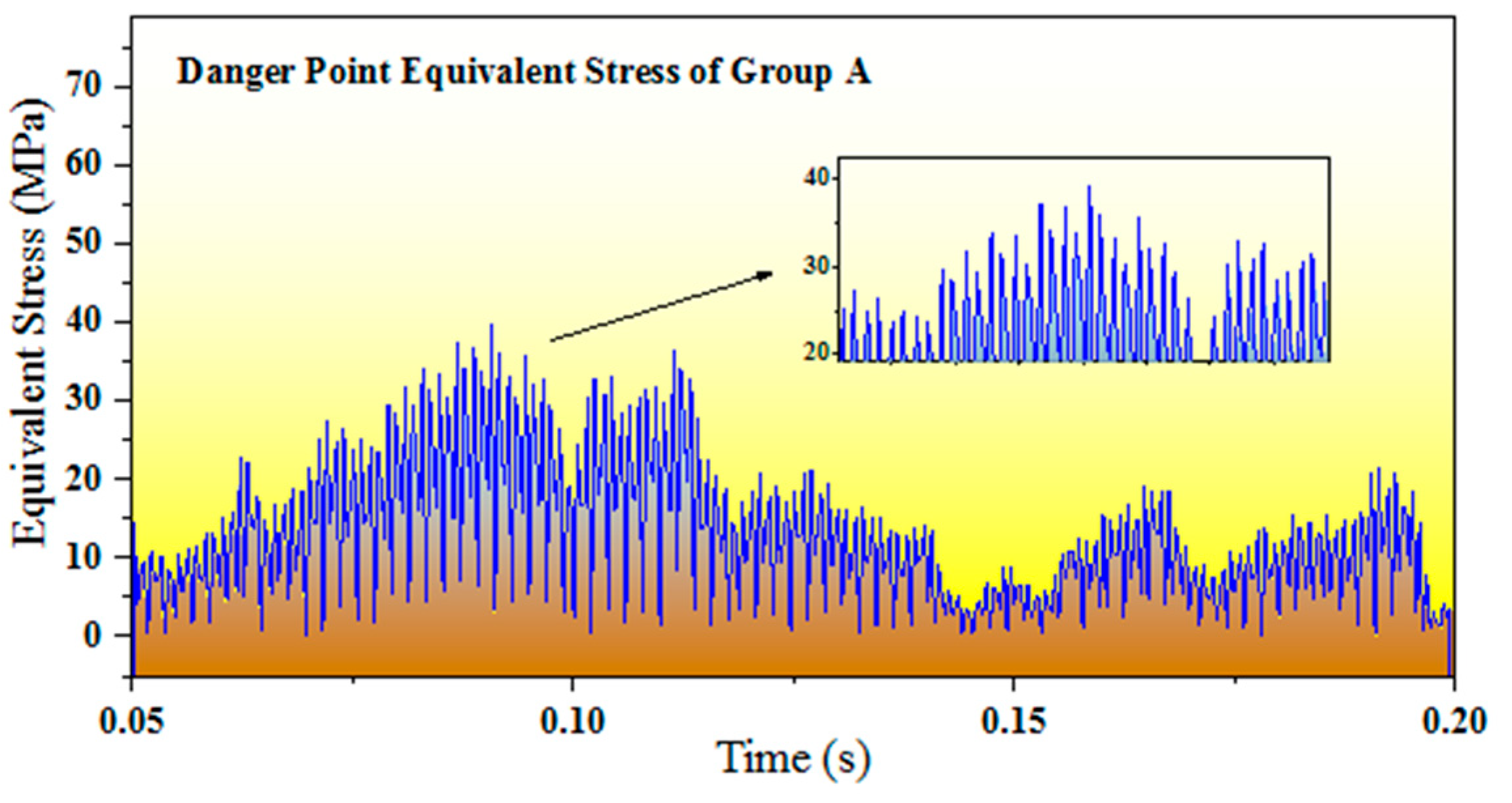
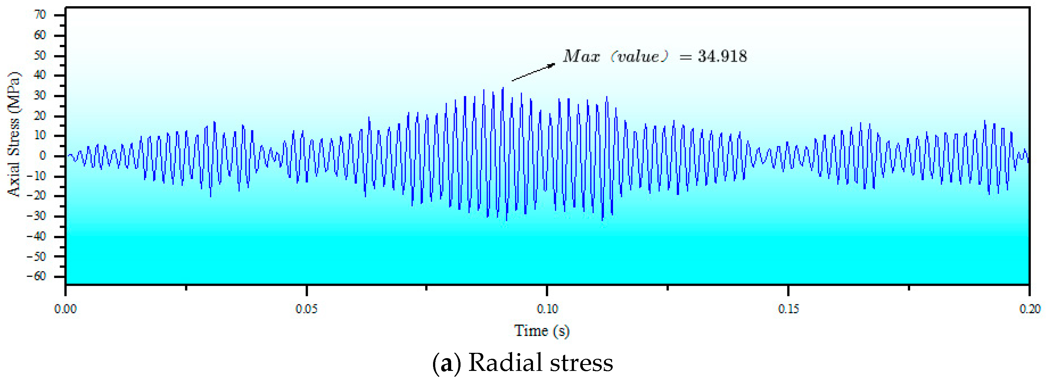
4.5.1. Group A Simulation Results

The simulation condition of Group A is external random load only, and the stress distribution cloud diagram of the Group A pipelines is shown in Figure 10. It can be seen from the figure that the stress danger points of Group A are located above and below the contact between the end supports and the pipe wall.
The equivalent stress curve of danger point A in the time domain is extracted, as shown in Figure 11, and the rainflow count is carried out, as shown in Figure 12. The result shows that the maximum equivalent stress of the danger point of group A is about 40 MPa.
Figure 13 shows the curve of radial, axial and circumferential stresses of the pipeline at the danger point of Group A. It can be seen from the figure that the radial, axial and circumferential stresses of the pipe wall have the same change trend with time, but in terms of magnitude, the axial and circumferential stresses reach 35 MPa and 11 MPa. The radial stress is less than 1 MPa. Therefore, the pipeline is mainly subjected to axial stress and circumferential stress under random vibration load, and the axial stress is the main stress, which provides a basis for the analysis of the pipeline vibration response in later tests.

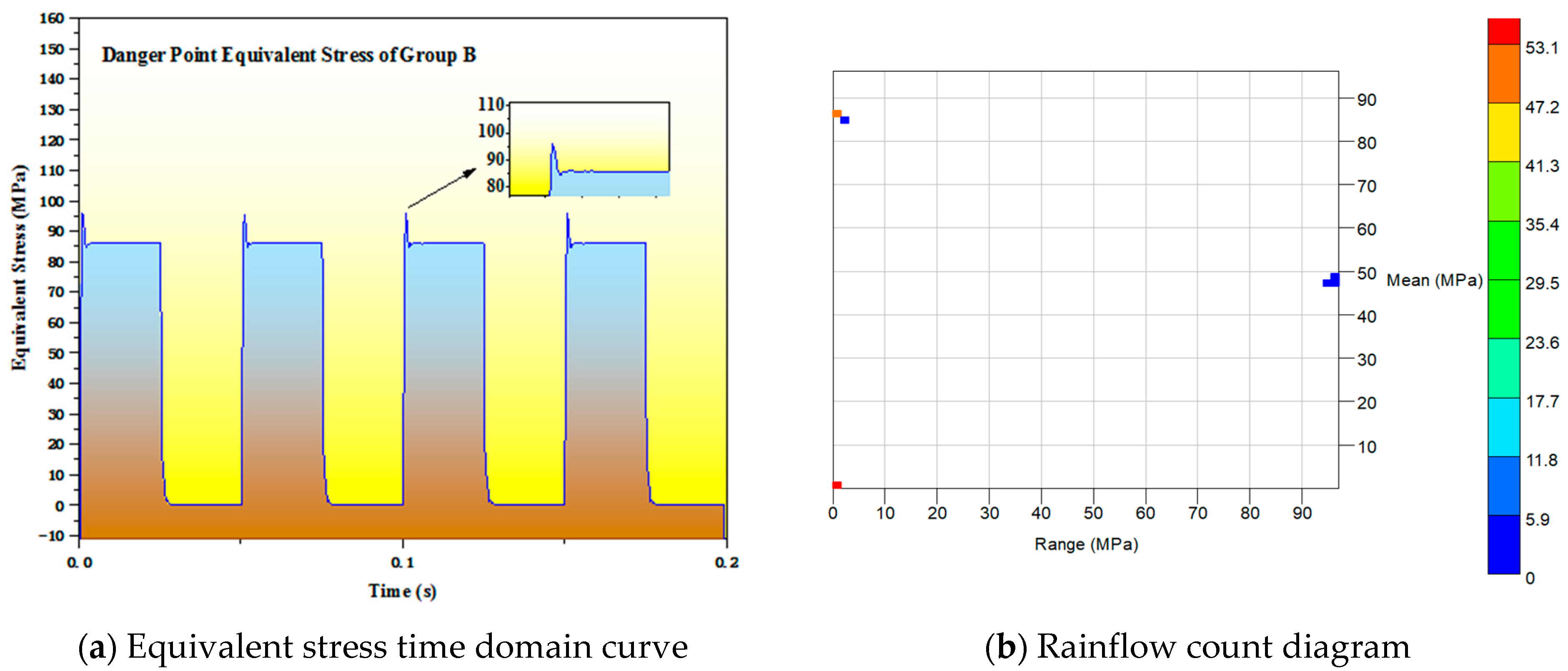
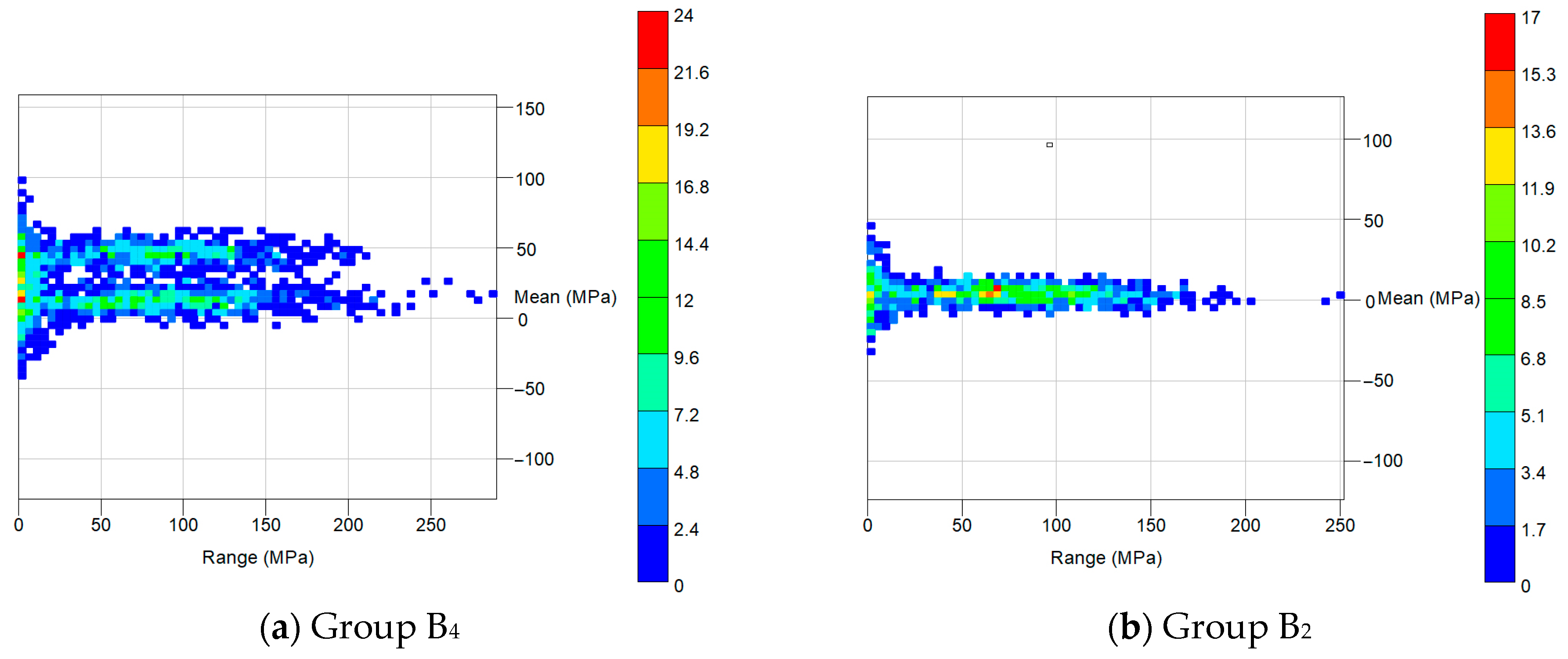
4.5.2. Group B Simulation Results

The simulation condition of Group B is fluid pulsating pressure only. By analyzing the results, the stress danger point of Group B is shown in Figure 14. As can be seen from the figure, the maximum pressure point appears at the inner corner of the pipe bend, which is the danger point of the vibration response in Group B. The equivalent stress time domain curve of the danger point is extracted, as shown in Figure 15a, and the rainflow-counting results are shown in Figure 15b. It can be seen that the equivalent stress of the danger point changes periodically. Its period is consistent with the fluid pressure pulsation. Similarly, the axial, circumferential and radial stresses of the point are extracted, and through comparative analysis, the circumferential stresses were much larger than the stresses in the other two directions. Therefore, it can be concluded that the circumferential stress is mainly the stress under the pulsating fluid pressure on the pipe wall.
At the same time, it can be seen that in the process of fluid pressure pulsation from low pressure to high pressure, the stress will have a shock value, and the shock amount is about 96 MPa. This is because the pressure changes from low pressure to high pressure instantaneously, and the pressure has a shock effect on the liquid-filled pipeline, which is the transient response of the pipeline. After a period of time, the stress at this point reaches a stable state. As can be seen from the rainflow-counting results, about half of the cyclic amplitude and mean stress values are 0 MPa, while the other half of the cyclic amplitude stress values are 0 MPa and the mean stress values are about 85 MPa. Only a few of the cyclic amplitude values of stress are relatively large, reaching 100 MPa, and the mean value of stress is 50 MPa (this part of the stress cycle is caused by impact).

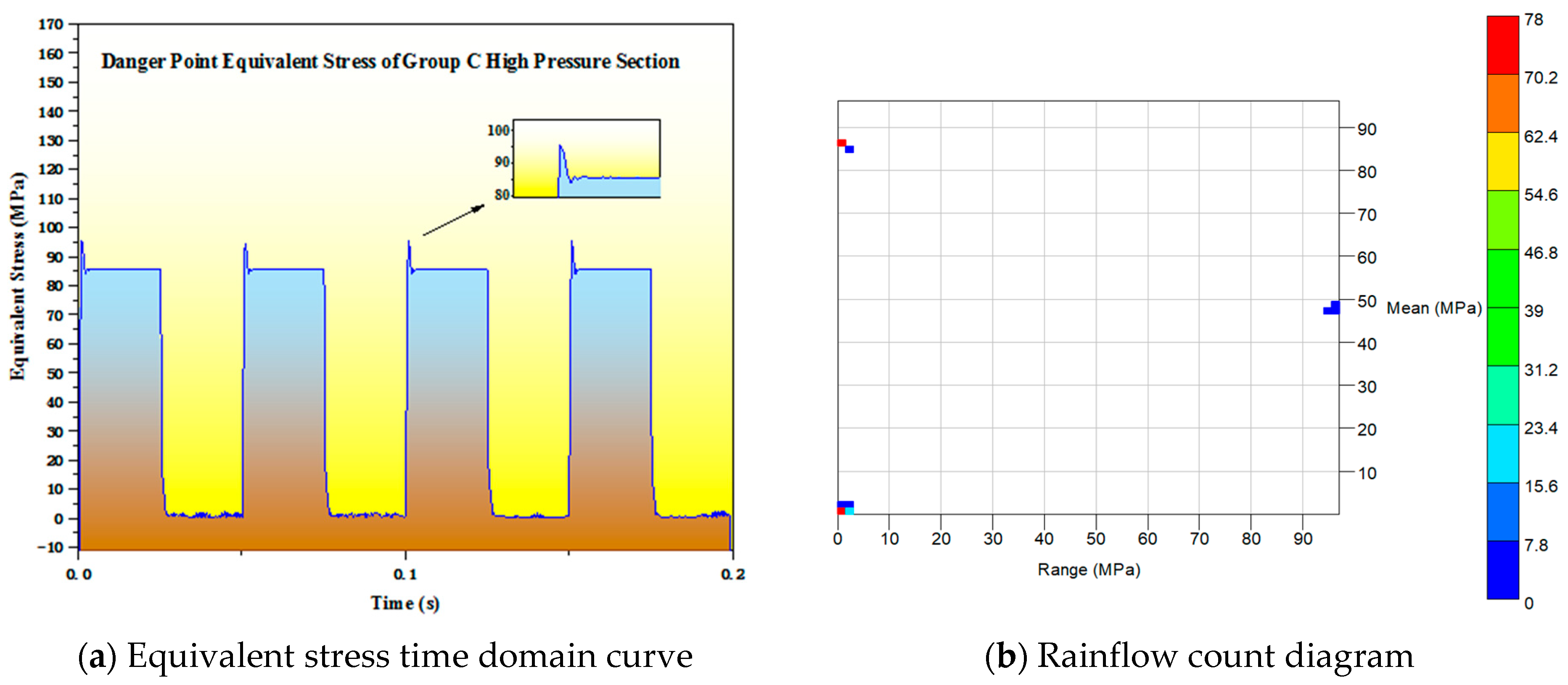
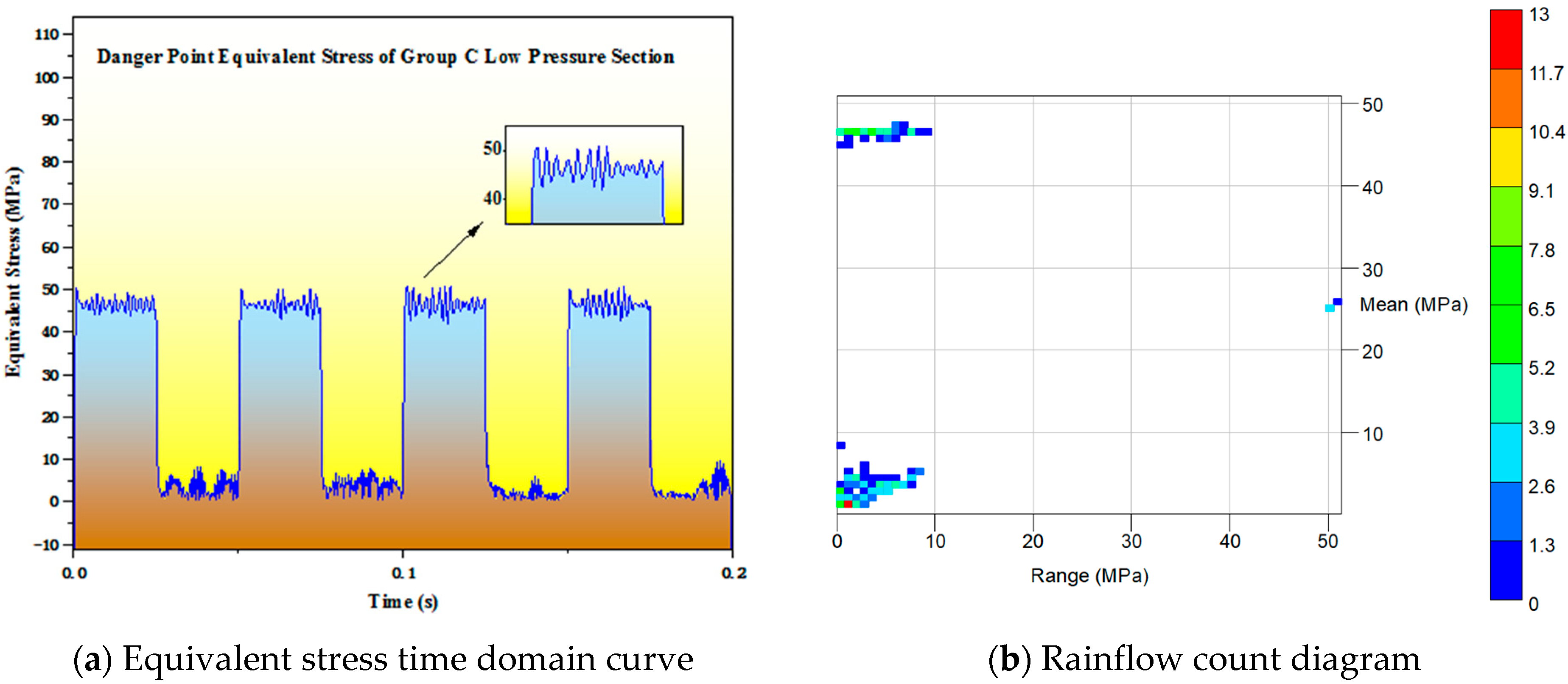
4.5.3. Group C Simulation Results

The simulation condition of Group C is that the load of the liquid-filled pipeline has both external random vibration and internal pulsating fluid pressure. By analyzing the simulation results of Group C, the conclusion is as follows: When the fluid pressure in the pipeline is in the high pressure section, as shown in Figure 6, the maximum point of equivalent stress on the pipe wall is located at the inner corner of the pipe bend, which is called danger point 1, as shown in Figure 16a. When the fluid pressure is in the low pressure section, as shown in Figure 6, the maximum equivalent stress point is located at the edge of the contact between the pipe and the support, which is called danger point 2, as shown in Figure 16b.
Therefore, the time domain equivalent stress curves of two danger points in the high-pressure and low-pressure sections of the Group C fluid were extracted, and the rainflow counts were performed on them, as shown in Figure 17 and Figure 18, respectively. The results show that when the fluid pressure is in the high pressure section, the maximum equivalent stress of danger point 1 of the Group C pipeline is 96 MPa; when the fluid pressure is in the low pressure section, the maximum equivalent stress of danger point 2 of the Group C pipeline is 52 MPa.

4.5.4. Comparison and Analysis of Simulation Results between Group A and Group B

The simulation condition of Group A is that the empty pipe is subjected to external random load, and the simulation condition of Group B is that the pipe filled with liquid is subjected only to fluid pulsation pressure. Through comparative analysis, it can be seen that the stress danger point of the Group A pipeline is located above and below the contact between the support at both ends of the pipeline, and the maximum equivalent stress is 40 MPa; the stress danger point of Group B pipeline is located at the inner corner of the pipe bend, and the maximum equivalent stress is 96 MPa. The vibration caused by the fluid pulsating pressure has a greater impact on the pipeline than that of the external random load. The simulation results of both Group A and Group B show that the radial stress is negligible compared with the axial and circumferential stress when the pipeline is subjected to external random load or pulsating pressure load. The main stress generated by the vibration response of the pipeline under external random load is the axial stress, while the main stress generated by the vibration response of the pipeline under pulsating pressure load is circumferential stress.

4.5.5. Comparison and Analysis of Simulation Results between Group A and Group C

The simulation condition of Group A is that the empty pipe is subjected to external random load, and the simulation condition of Group C is that the pipe is subjected to both external random load and fluid pulsating pressure. Through comparative analysis, it can be seen that when the fluid pressure of Group C is in the low pressure section, the stress danger point is located above and below the contact between the support at both ends of the pipeline, that is, danger point 2. The maximum equivalent stress is 52 MPa, which is consistent with the stress danger point of the Group A simulation results. Group C simulation conditions aggravate the vibration response of the pipeline due to the presence of fluid pulsating pressure.

4.5.6. Comparison and Analysis of Simulation Results between Group B and Group C

The simulation condition of Group B is that the pipeline filled with liquid is subjected to only the fluid pulsation pressure, and the simulation condition of Group C is that the pipeline is subjected to both the external random load and the fluid pulsation pressure. Through comparative analysis, it can be seen that when the fluid pressure of Group C is in the high-pressure section, the stress danger point is located at the inner corner of the pipe bend, that is, danger point 1, and the maximum equivalent stress is 96 MPa, which is consistent with the stress danger point of the simulation results of Group B. By comparing the time domain curve and rainflow count diagram (Figure 17) of the equivalent stress at danger point 1 in the high-pressure section of Group C with that of Group B (Figure 15), it can be seen that the stress generated by random vibration at this danger point is much smaller than that of the fluid pulsation pressure. In comparison, the influence of external random vibration on the pipeline is very limited compared to the simulation conditions of Group B.
Simulation analysis provides the research basis for subsequent experimental research, mainly as follows:
  • Under external random vibration, the stress danger point of the pipeline is located at the support contact pipe wall at both ends; furthermore, the radial stress can be ignored, and the axial stress is the main stress generated by the pipeline vibration.
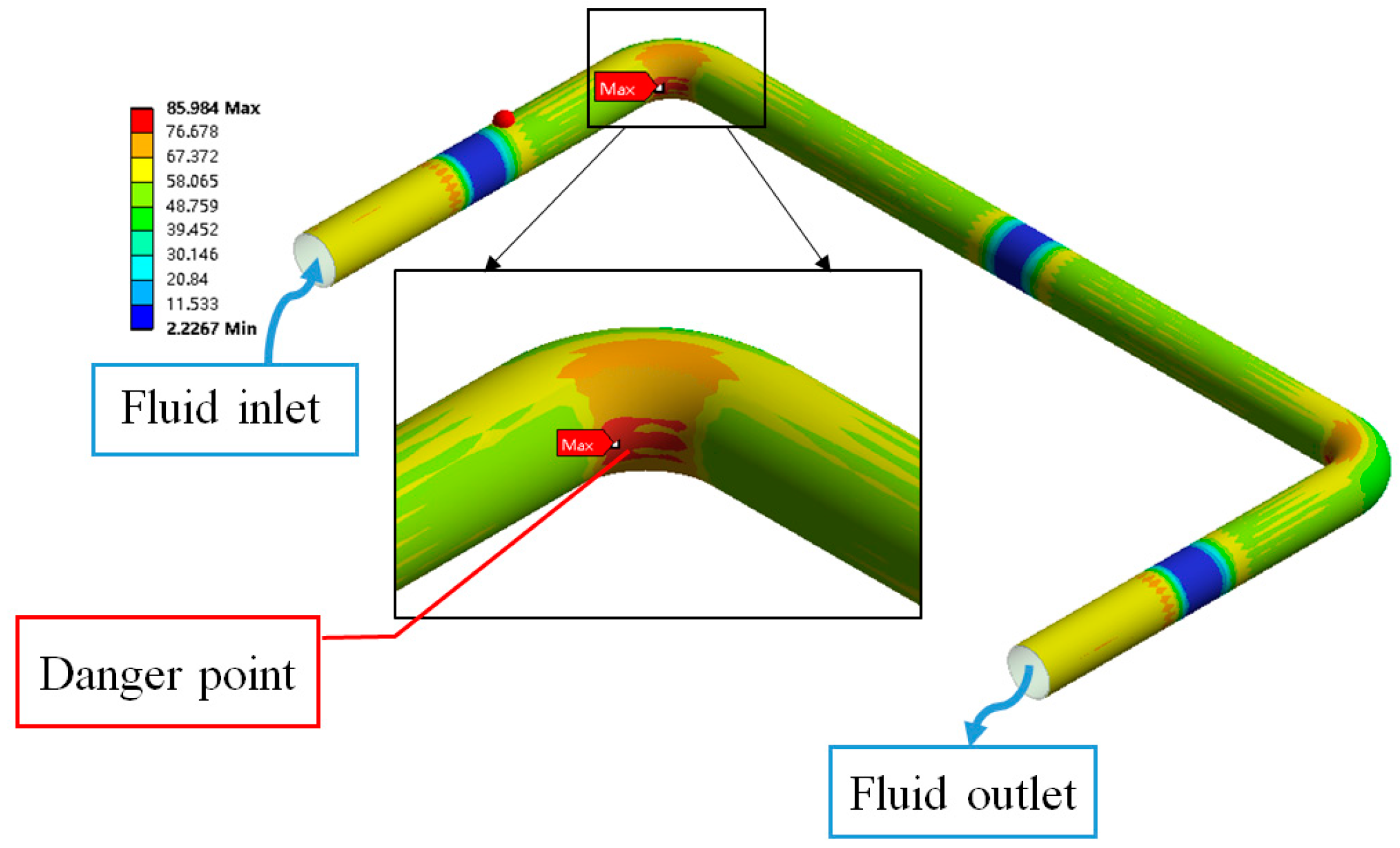
  • Under the effect of internal fluid pulsation pressure, the stress danger point of the pipeline is at the inner corner of the pipeline. The radial stress can also be ignored, and the circumferential stress is the main stress generated by the pipeline vibration.

5. Experimental Investigation on Aircraft Liquid-Filled Pipelines

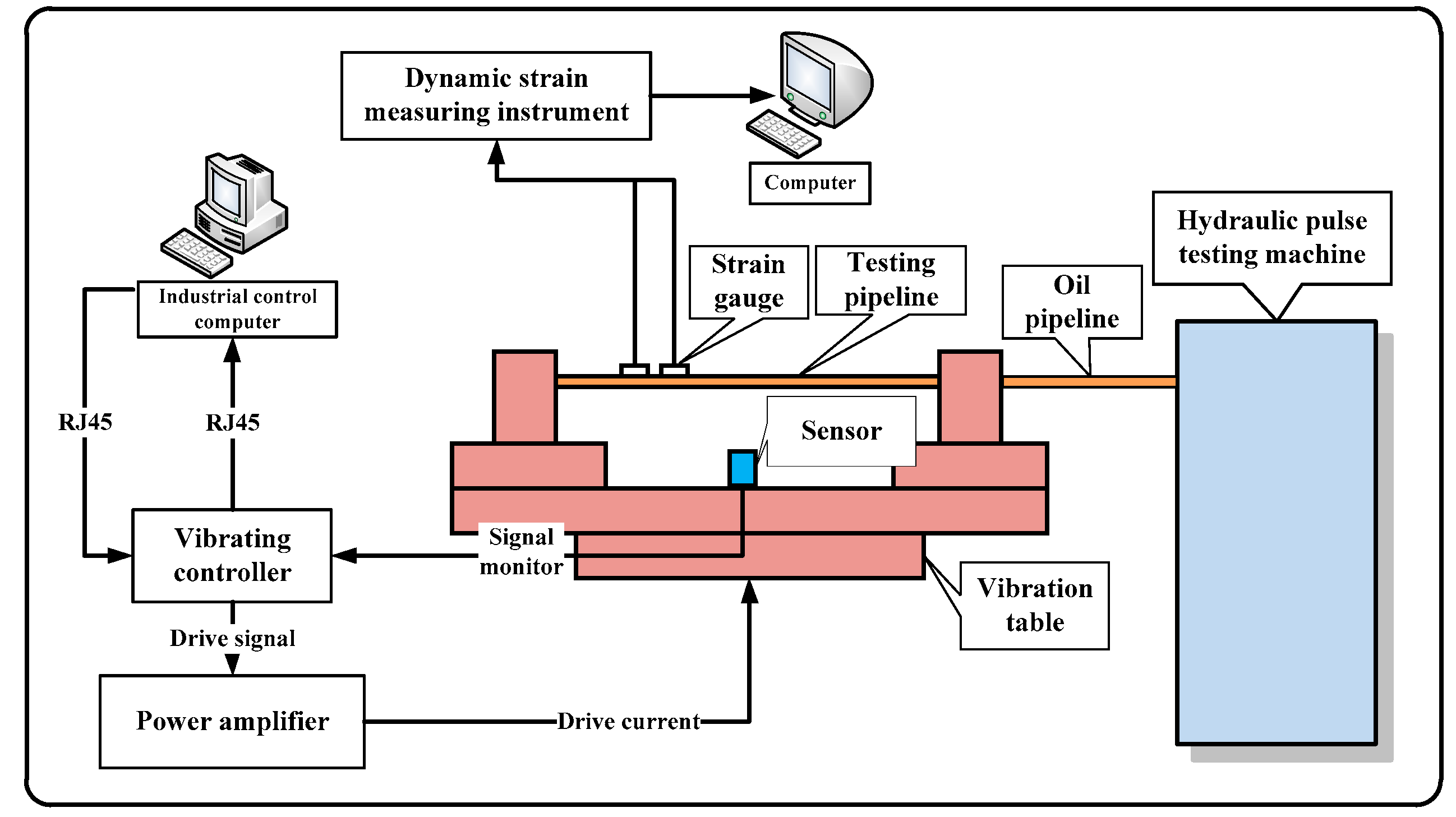
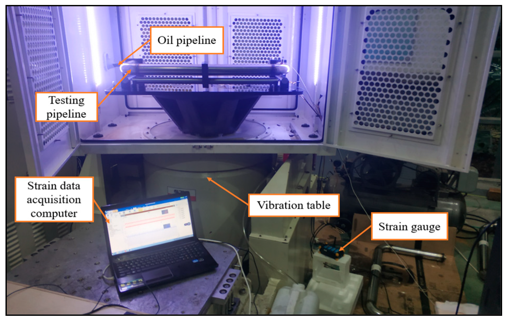
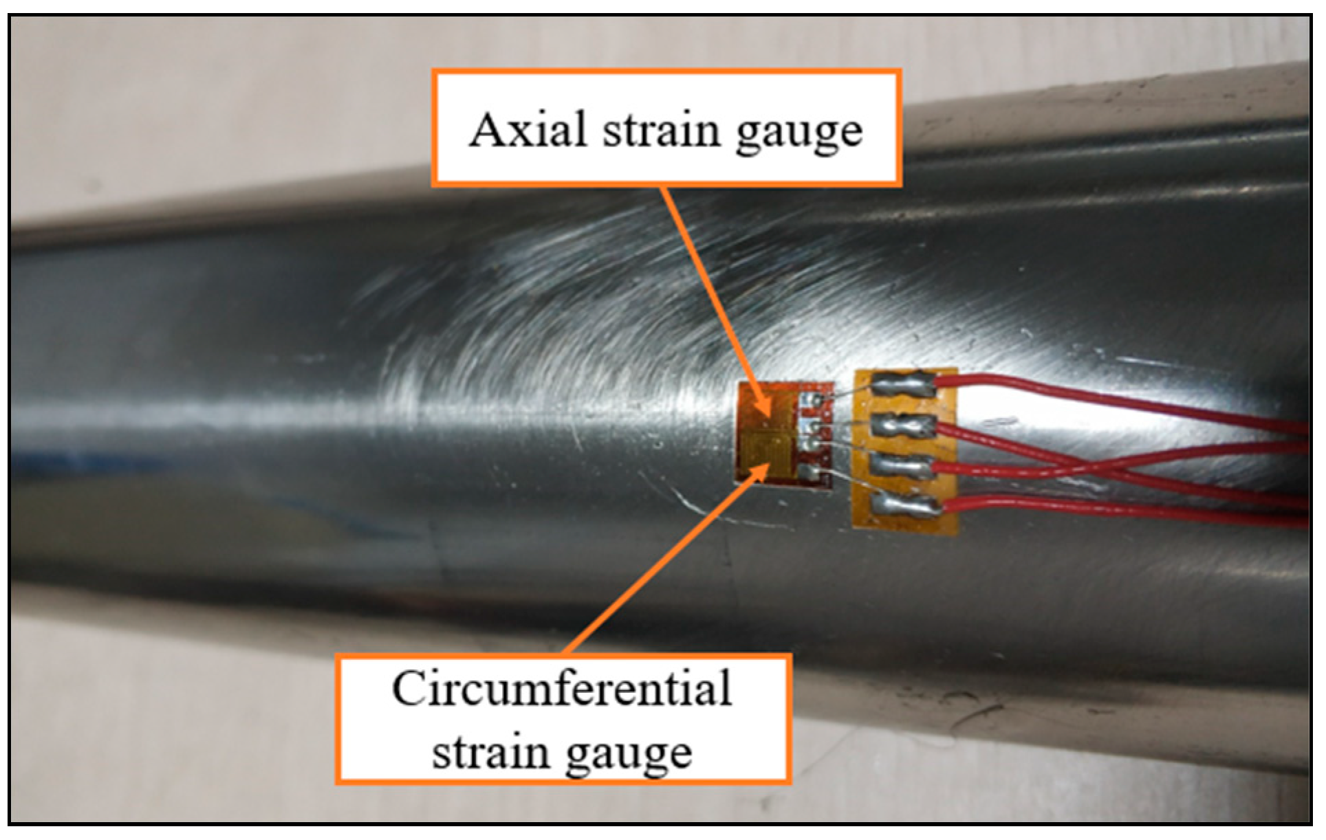
5.1. Experimental Set-Up

The test system is a closed-loop vibration control system, the schematic diagram of which is shown in Figure 19. The vibration controller is a non-Gaussian NRVCS vibration controller, which can control the kurtosis and meet the requirements of the super-Gaussian random vibration in the test. A Donghua DH5908 wireless dynamic strain gauge with 4 channels was selected as the dynamic strain gauge. Strain gauges with high resistance value were selected. In this test, a 350 Ω high-resistance foil strain gauge was selected, and the half-bridge method with a temperature compensation plate was adopted to eliminate the influence of temperature.

5.2. Preparation of Specimens and Grouping of Test Conditions

The vibration response analysis of liquid-filled pipelines was considered from three aspects. Firstly, the influence of super-Gaussian vibration on the vibration response of pipelines was studied and the random vibration kurtosis of the test was divided into three classes: 3, 5, 7. Secondly, the influence of different operating conditions of the liquid-filled pipeline on the vibration response of the pipeline was investigated. Finally, the influence of different wall thicknesses on the vibration response of liquid-filled pipelines was investigated. Table 3 shows the grouping of tests.
According to the results measured by the natural frequency test of the liquid-filled pipeline in the early stage, the first 8 natural frequencies of the pipeline are all within 500 Hz. Therefore, in order to generate a large vibration response of the pipeline, so as to generate a larger strain value on the pipe wall and reduce the error caused by external environmental disturbance, the random vibration frequency range selected in this test is 20–500 Hz. The root mean square acceleration is 6.9 g; the liquid pulsation frequency provided by the hydraulic testing machine is 0.5 Hz, the maximum pressure value of the liquid pulsation is 5 MPa and the minimum pressure value is 0.5 MPa. According to the analysis of the previous simulation results, it can be seen that the pulsating pressure of the fluid has a greater impact on the vibration of the pipeline than the external random vibration. Therefore, during the test, the U-shaped pipe should be avoided from breaking at the bend, and the bend of the U-shaped pipe is designed to be thicker than the wall of the straight pipe. The test in this paper mainly studies the vibration stress response analysis at the edge of the contact between the pipe and the fixed support (the stress danger point 2 in the simulation). So, the strain gauge mainly measures the strain at this point, and the directions are axial strain and circumferential strain. Figure 20 shows the fluid–structure interaction vibration response test system of the liquid-filled pipeline, and the axial and circumferential strain gauge patch diagram of the test pipeline is shown in Figure 21.

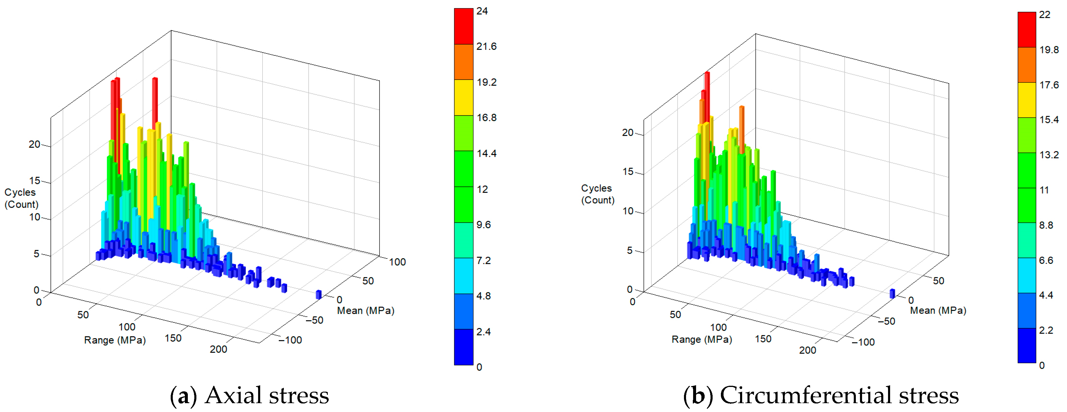
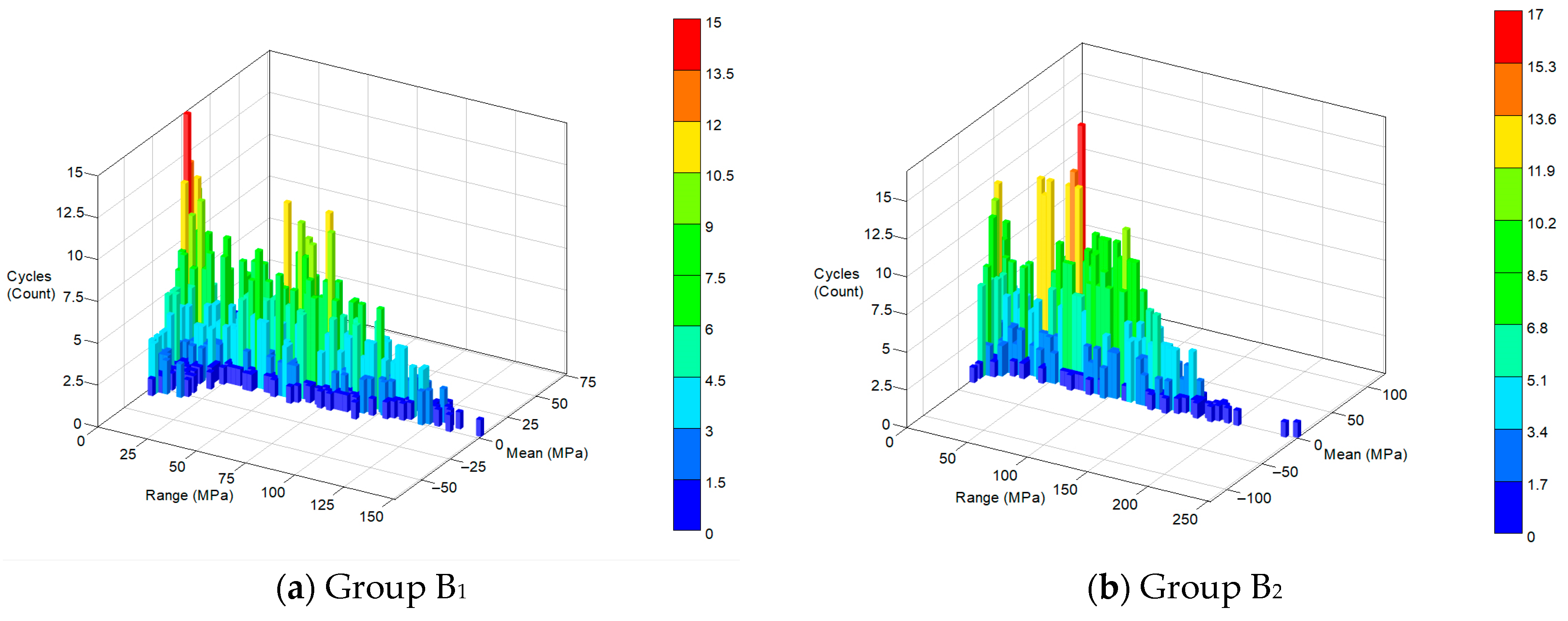
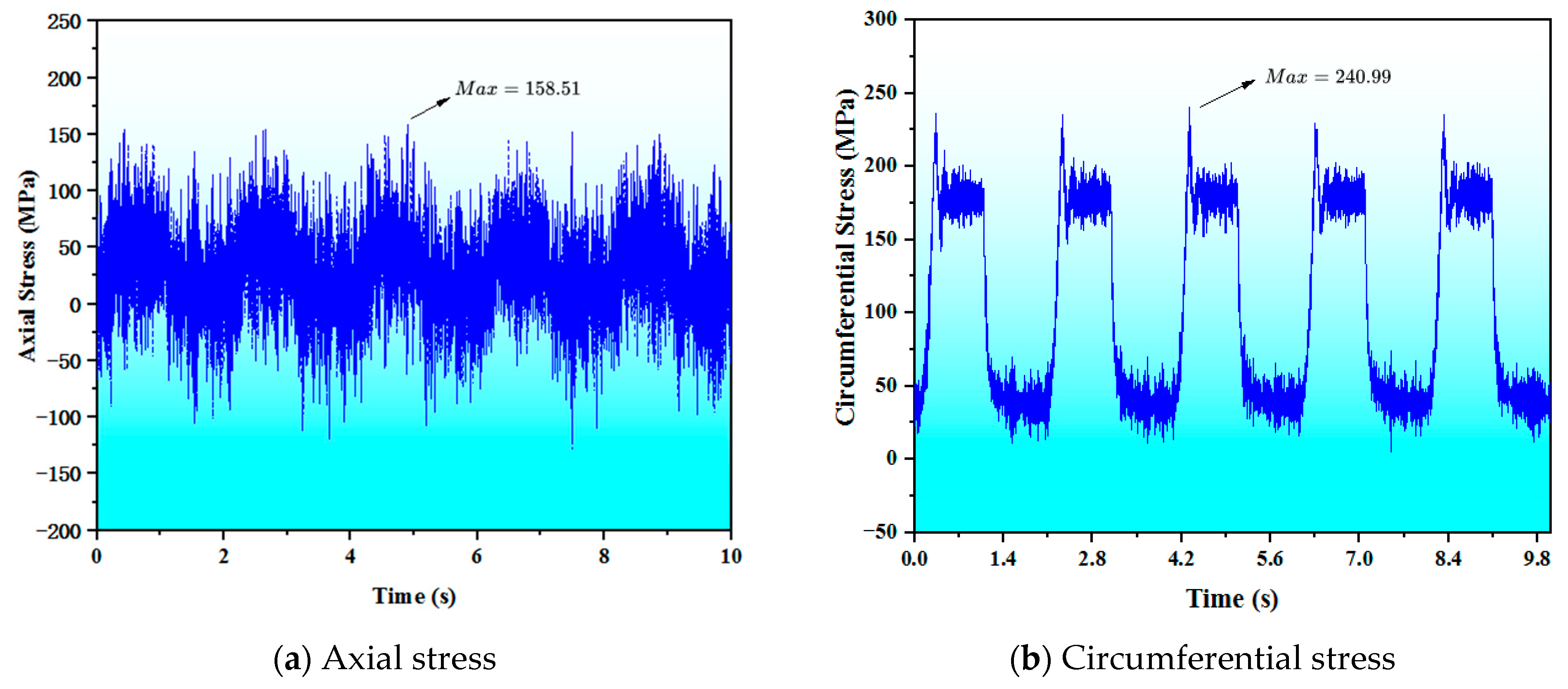
5.3. Experiment Result Analysis

5.3.1. Test Results Analysis of Group A

The test conditions of Group A all involved being subjected to external random load, and three control tests were set up as A1, A2 and A3, respectively. The vibration signal kurtosis values of the three groups of random load were 3, 5 and 7, respectively. The purpose of setting up Group A was to explore the sensitivity of the pipeline vibration response to the kurtosis value of the non-Gaussian random vibration load. The axial and circumferential strain signals of the pipeline were collected by the strain gauge and converted to stress by calculation. MATLAB R2022a software was used to solve the kurtosis value of the axial and circumferential time domain stresses.
As can be seen from Table 4, when the input signal is Gaussian random vibration, the stress response of the pipeline at the danger point is close to Gaussian distribution; that is, when the input excitation signal kurtosis is 3, the kurtosis of the stress response is attenuated to a certain extent, but it is still close to Gaussian distribution. When the excitation signal is super-Gaussian random vibration, that is, the kurtosis value is 5 or 7, the stress response of the pipeline at the danger point shows super-Gaussian characteristics. With the increase in kurtosis, the kurtosis attenuation degree of stress response is greater. Meanwhile, it was found that the kurtosis attenuation of axial stress was more severe than that of circumferential stress.
Figure 22 shows the rainflow count diagram of axial stress and circumferential stress in group A1, and Figure 23 shows the rainflow count diagram of axial stress in groups A2 and A3. It can be seen from the figure that the maximum axial stress value of group A1 is 150 MPa, which is larger than the maximum circumferential stress value of 26 MPa. Therefore, it can be inferred that under the load of external random vibration only, the axial stress amplitude of the pipeline is much larger than the circumferential stress amplitude, the axial stress plays a decisive role in the vibration response stress of the pipeline. Therefore, the axial stress of the contact position between the pipe and the support is worth paying attention to under the condition of external random vibration. Comparing the axial stress of groups A1, A2 and A3, it can be seen that when the applied load excitation is super-Gaussian random vibration, the stress amplitude of the pipeline at the danger point increases, so when the external load presents super-Gaussian characteristics, the vibration response of the pipeline will be increased.

5.3.2. Test Results Analysis of Group B

Group B was set up to compare the vibration response analysis of four different working conditions of the pipeline. First, the results of groups B1 and B2 were analyzed; that is, an empty pipeline subjected to external random load and a liquid-filled pipeline subjected to external random load (hydraulic pressure is 0 MPa), respectively. Figure 24 shows the results of the rainflow counting of the axial stress at the danger points of groups B1 and B2.
As can be seen from Figure 24, the maximum value of the axial stress of the danger point in Group B1 is 150 MPa and the maximum value of the axial stress of the danger point in Group B2 is 250 MPa. The maximum value of the axial stress rainflow number of the danger point in Group B2 is larger than that in Group B1. The results show that the vibration response of the pipeline filled with liquid is more intense than that of the empty pipeline under random vibration load.
Figure 25 shows the time domain response curves of axial and circumferential stress at the danger points of group B3. The stress of the group B3 liquid-filled pipeline presents a periodic change, and there is a pulse pressure at the position of high and low pressure change. At the same time, it can be observed that the circumferential stress at the danger point of the liquid-filled pipeline is significantly greater than the axial stress. The axial stress is about 0.3 times the circumferential stress and the Poisson’s ratio of stainless steel is also 0.3. According to the definition of Poisson’s ratio, when the linear elastic material is stretched and deformed in one direction, the strain is ε . The strain perpendicular to the direction is ε 1 . The negative value of the ratio of ε 1 and ε is called Poisson’s ratio. It can be inferred that the pulsating pressure of the fluid on the pipe will generate only circumferential stress, while the axial stress will be generated by the Poisson’s ratio effect of the materials. When investigating the response of the pulsating pressure of the fluid to the vibrational stress of the pipe, only the circumferential stress of the pipe should be considered.
Figure 26 shows the time domain response curves of axial stress and circumferential stress of the Group B4 liquid-filled pipeline at the danger point under the combined action. From the previous analysis, it can be seen that the axial stress of the liquid-filled pipeline is more sensitive to random vibration, and the circumferential stress is more sensitive to the fluctuating pressure of the fluid, which is confirmed by Figure 22 and Figure 25.
The rainflow count of the axial stress of Group B4 can be compared with the rainflow count of the axial stress of the liquid-filled pipeline in Group B2, which only has a random vibration effect, as shown in Figure 27. As can be seen from the figure, the maximum axial stress amplitude of Group B4 is 300 MPa, while that of Group B2 is 250 MPa. At the same time, due to the presence of fluid pressure, the average axial stress of Group B4 is greater than that of Group B2. Therefore, it can be seen that the vibration response of the pipeline under the combined action is more intense than that under the external random vibration action alone (fluid pressure is 0 MPa).

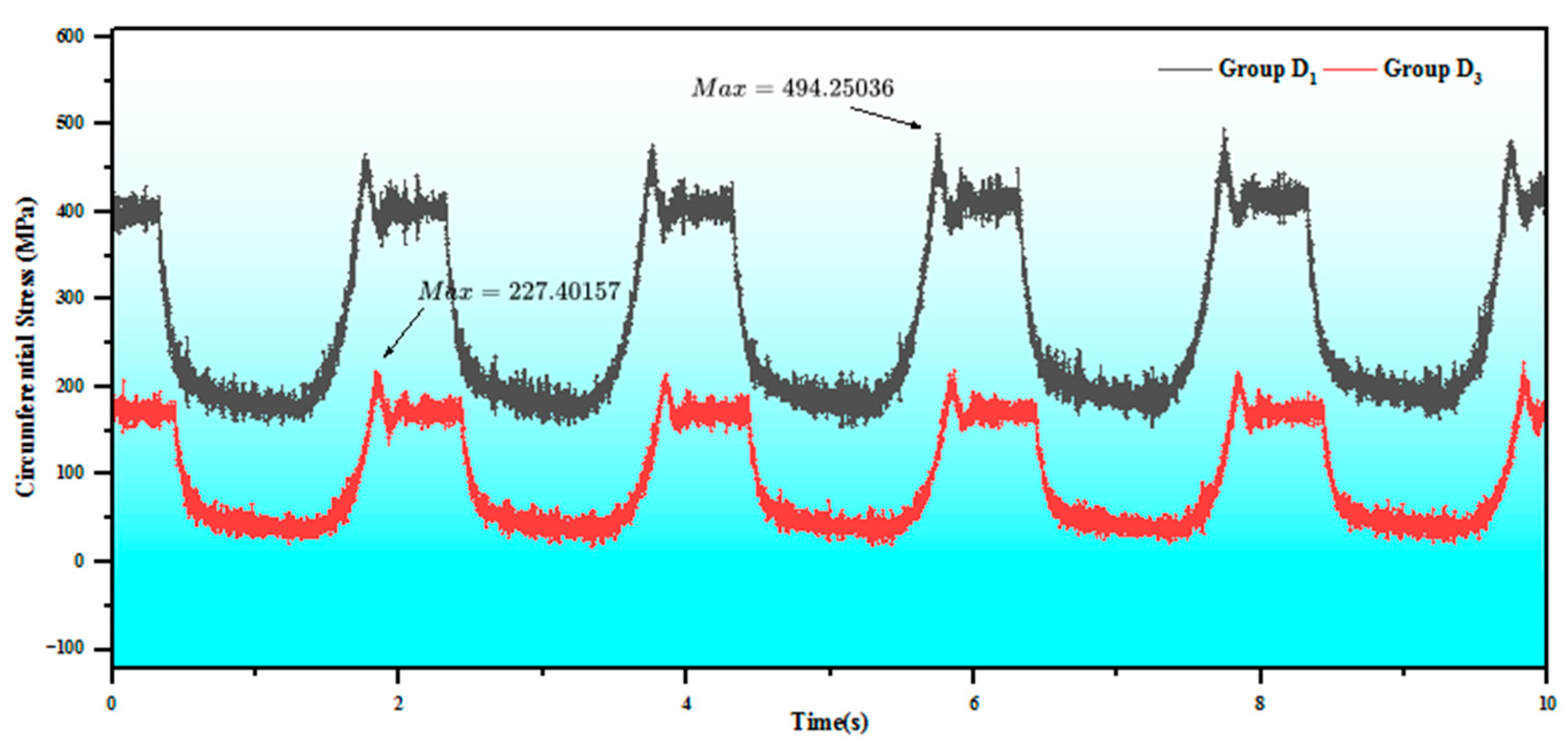
5.3.3. Test Results Analysis of Group C and D

The purpose of setting up groups C and D is to study the influence of wall thickness of liquid-filled pipelines on vibration response. The working condition of Group C is an empty pipe with random vibration only, and Group D is combined action.
According to the previous test verification and analysis, for Group C, the axial stress plays a leading role compared with the circumferential stress. Therefore, the axial stress of Group C was extracted and the rainflow count was carried out to obtain the maximum value of the stress, as shown in Table 5. As can be seen from the table, as the wall thickness increases, the maximum axial value of the pipe shows a decreasing trend, but the degree of reduction becomes smaller and smaller. After a wall thickness of 0.7 mm, the reduction in the stress response is insensitive to the increase in the wall thickness, which is called the critical value of the pipe wall thickness. After the critical value, as the pipe wall thickness increases, the stress decay of the vibration response gradually decreases and tends to be stable.
For Group D, it was verified by analysis that the axial stress and the circumferential stress have the same rule as that of Group B, so only the circumferential stress was analyzed. Figure 28 shows the time domain curve of circumferential stress of Group D1 and Group D3, and Figure 26b shows the Group D2. The comparative analysis shows that the maximum circumferential stress of 0.5 mm pipe wall thickness reaches 475 MPa, while the maximum circumferential stress of 1.4 mm wall thickness, 1 mm wall thickness and 0.7 mm wall thickness are all around 225 MPa. Similar to the test results of Group C, when the wall thickness reaches 0.7 mm, the decrease in the stress response is not sensitive to the increase in the wall thickness. Meanwhile, the hysteresis phenomenon is observed in Figure 28, that is, the stress on the pipe wall cannot return to the initial value after one cycle, which is reflected in the increasing trend of the mean stress in the figure. This is due to the plastic deformation of group D2, where the tube wall is too thin and the excessive stress on the tube wall exceeds the elastic range of the material.

6. Conclusions

Through simulation analysis and experimental research, this paper investigates and analyses the fluid–structure interaction vibration stress response of liquid-filled pipelines under the superimposed effects of external random load and internal fluid pulsation. By analyzing the stress response of the liquid-filled pipeline at danger points, the influence mechanism and rule of different kurtoses, different working conditions and different pipe wall thicknesses on the fluid–structure interaction vibration stress response of the liquid-filled pipeline were investigated, and the following conclusions can be drawn:
  • The danger point of the vibration response stress of the aircraft liquid-filled pipeline under the action of external random load is located above and below the contact between the support at both ends of the pipeline. The danger point of the vibration response stress under the action of internal fluid pulsation pressure is located at the inner corner of the pipe bend, so the damping device should be added in these two parts to reduce the vibration stress when designing the aircraft pipeline.
  • The vibration response stress of the aircraft liquid-filled pipe under external random load is mainly axial stress, while the vibration response stress under internal fluid pulsation pressure is mainly circumferential stress, and the radial stress generated by both loads can be ignored, which provides a basis for aircraft vibration response analysis.
  • Compared with the Gaussian random vibration load, the super-Gaussian random vibration load will have a larger response to the vibration of the aircraft liquid-filled pipe. Therefore, when carrying out the anti-fatigue design of the aircraft liquid-filled pipe, whether the external load has super-Gaussian characteristics should be fully considered.
  • Under the same external load, the vibration response of the aircraft pipe is more intense than that of the empty pipe after it is filled with liquid. In the anti-fatigue design and simulation test of the aircraft duct, in order to obtain real and reliable results, the relevant design and test should be carried out considering the presence of liquid.
  • The wall thickness of aircraft piping filled with liquid has a critical value. When the wall thickness is larger than this critical value, the stress decay of the vibration response gradually decreases with increasing wall thickness and tends to be stable under the same working conditions. Therefore, when designing aircraft piping, it is not the case that the thicker the wall thickness, the better. The appropriate wall thickness of the pipe should be selected by considering the economy, aircraft load capacity and vibration stress response of the pipe. At the same time, if the wall thickness of the pipe is below a certain value, plastic deformation will occur due to the pulsating pressure of the fluid, which should be taken into account when designing the aircraft pipe.
These conclusions can provide guidance for aircraft piping design, vibration reduction design, simulation testing and fatigue life analysis. Next, based on the research in this paper, the method proposed in this paper can be used to simulate and verify the actual equipment according to the measured vibration load signal and fluid pulsating pressure signal on the aircraft engine pipeline.

Author Contributions

Conceptualization, C.C. and Y.J.; methodology, L.Z.; writing—original draft, C.C. and L.Z.; writing—review & editing, Y.J.; visualization, C.C. All authors have read and agreed to the published version of the manuscript.

Funding

This research received no external funding.

Institutional Review Board Statement

Not applicable.

Informed Consent Statement

Not applicable.

Data Availability Statement

The original contributions presented in the study are included in the article, further inquiries can be directed to the corresponding author.

Conflicts of Interest

The authors declare no conflicts of interest.

References

  1. Lian, J.; Yang, X.; Wang, H. Propagation characteristics analysis of high-frequency vibration in pumped storage power station based on a 1D Fluid-Structure Interaction model. J. Energy Storage 2023, 68, 107869. [Google Scholar] [CrossRef]
  2. Liu, Y.; Wei, J.; Du, H.; He, Z.; Yan, F. An Analysis of the Vibration Characteristics of an Aviation Hydraulic Pipeline with a Clamp. Aerospace 2023, 10, 900. [Google Scholar] [CrossRef]
  3. Zhang, T.; Cui, J. Analytical Method for Fluid-Structure Interaction Vibration Analysis of Hydraulic Pipeline System with Hinged Ends. Shock. Vib. 2021, 2021, 8846869. [Google Scholar] [CrossRef]
  4. Zhang, Y.; Ding, L.; Qi, M.; Bei, G. Numerical Analysis of Dynamic Characteristics of Thermowell Based on Two-Way Thermo-Fluid-Structure Interaction. Shock. Vib. 2021, 2021, 7759673. [Google Scholar] [CrossRef]
  5. Su, Y.; Gong, W. Research on vibration characteristics of rocket engine flow pipeline. Aircr. Eng. Aerosp. Technol. 2024, 96, 387–402. [Google Scholar] [CrossRef]
  6. Liang, Z.; Guo, C.; Wang, C. The Connection between flow pattern evolution and vibration in 90-degree pipeline: Bidirectional fluid-structure interaction. Energy Sci. Eng. 2022, 10, 308–323. [Google Scholar] [CrossRef]
  7. Liu, E.; Wang, X.; Zhao, W.; Su, Z.; Chen, Q. Analysis and Research on Pipeline Vibration of a Natural Gas Compressor Station and Vibration Reduction Measures. Energy Fuels 2021, 35, 479–492. [Google Scholar] [CrossRef]
  8. Qu, W.; Zhang, H.; Li, W.; Sun, W.; Zhao, L.; Ning, H. Influence of Support Stiffness on Dynamic Characteristics of the Hydraulic Pipe Subjected to Basic Vibration. Shock. Vib. 2018, 2018, 4035725. [Google Scholar] [CrossRef]
  9. Beatty, M.; Elías-Zúñiga, A. Stress-softening effects in the vibration of a non-Gaussian rubber membrane. Math. Mech. Solids 2003, 8, 481–495. [Google Scholar] [CrossRef]
  10. Jiang, Y.; Tao, J.; Zhang, Y.; Yun, G. Fatigue life prediction model for accelerated testing of electronic components under non-Gaussian random vibration excitations. Microelectron. Reliab. 2016, 64, 120–124. [Google Scholar] [CrossRef]
  11. Wang, Z.; Song, J. Equivalent linearization method using Gaussian mixture (GM-ELM) for nonlinear random vibration analysis. Struct. Saf. 2017, 64, 9–19. [Google Scholar] [CrossRef]
  12. Zheng, R.; Chen, H.; Vandepitte, D.; Luo, Z. Multi-exciter stationary non-Gaussian random vibration test with time domain randomization. Mech. Syst. Signal Process. 2019, 122, 103–116. [Google Scholar] [CrossRef]
  13. Ren, S.; Chen, H.; Zheng, R. Modified time domain randomization technique for multi-shaker non-stationary non-Gaussian random vibration control. Mech. Syst. Signal Process. 2024, 213, 111311. [Google Scholar] [CrossRef]
Figure 1. Research proposal of fluid–structure interaction vibration response analysis of liquid–filled pipelines.
Applsci 14 08008 g001
Figure 2. An aircraft engine pipeline layout diagram.
Applsci 14 08008 g002
Figure 3. U-shaped pipe diagram.
Applsci 14 08008 g003
Figure 4. Model of liquid-filled pipeline.
Applsci 14 08008 g004
Figure 5. Generation of random loads. (a) The power spectral density function of the acceleration load. (b) The time domain signal of the acceleration load.
Applsci 14 08008 g005
Figure 6. The pulsating pressure time domain signal load.
Applsci 14 08008 g006
Figure 7. Grid division of the pipeline.
Applsci 14 08008 g007
Figure 8. Bidirectional fluid–structure interaction data transfer mode.
Applsci 14 08008 g008
Figure 9. Boundary conditions for simulation of liquid–filled pipelines.
Applsci 14 08008 g009
Figure 10. Stress distribution deprogram of Group A pipeline.
Applsci 14 08008 g010
Figure 11. Group A danger point equivalent stress time domain curve.
Applsci 14 08008 g011
Figure 12. Group A equivalent stress rainflow count chart of danger points.
Applsci 14 08008 g012
Figure 13. Response curve of stress in each direction at danger point of Group A pipelines.
Applsci 14 08008 g013aApplsci 14 08008 g013b
Figure 14. Group B stress danger point diagram.
Applsci 14 08008 g014
Figure 15. Group B danger point equivalent stress.
Applsci 14 08008 g015
Figure 16. Danger point in Pipeline C.
Applsci 14 08008 g016
Figure 17. Equivalent stress at danger point 1 of high pressure section of Group C pipeline.
Applsci 14 08008 g017
Figure 18. Equivalent stress at danger point 1 of low pressure section of Group C pipeline.
Applsci 14 08008 g018
Figure 19. Pipeline vibration response test device schematic diagram.
Applsci 14 08008 g019
Figure 20. An aircraft engine pipeline layout diagram.
Applsci 14 08008 g020
Figure 21. U-shaped pipe diagram.
Applsci 14 08008 g021
Figure 22. Group A1 danger point stress rainflow count.
Applsci 14 08008 g022
Figure 23. Group A2 and A3 danger point axial stress rainflow count.
Applsci 14 08008 g023
Figure 24. Group B1 and B2 danger point axial stress rainflow count.
Applsci 14 08008 g024
Figure 25. Time domain response curves of axial and circumferential stress of group B3 pipeline danger points.
Applsci 14 08008 g025
Figure 26. The time domain response curves of axial stress and circumferential stress of group B4.
Applsci 14 08008 g026
Figure 27. Group B4 and B2 danger point axial stress rainflow count.
Applsci 14 08008 g027
Figure 28. Time domain curve of circumferential stress at danger points of Group D1 and Group D3 pipelines.
Applsci 14 08008 g028
Table 1. Simulation group of fluid–structure interaction vibration response of liquid-filled pipelines.
Simulation GroupSimulation Condition
Aonly stimulated by external random excitation
Bonly stimulated by the pulsating fluid pressure in the pipe
Ccombined action
Table 2. Experimental material properties.
MaterialMaterial
Density (kg/m3)
Young’s
Modulus (GPa)
Poisson’s
Ratio
Tensile
Limit (MPa)
Dynamic
Viscosity (Pa s)
SUS30478502040.3520None
Steel78502000.3250None
Oil8724.80None0.0279
Table 3. Pipeline vibration response test group.
GroupOil-FilledKurtosisRandom LoadPulsating Liquid PressurePipe Wall Thickness
A1No3YesNo0.7 mm
A2No5YesNo0.7 mm
A3No7YesNo0.7 mm
B1(A1)No3YesNo0.7 mm
B2Yes3Yes0 Mpa0.7 mm
B3Yes3No0.5–5 Mpa0.7 mm
B4Yes3Yes0.5–5 Mpa0.7 mm
C1No3YesNo0.5 mm
C2(A1)No3YesNo0.7 mm
C3No3YesNo1 mm
C4No3YesNo1.4 mm
D1Yes3Yes0.5–5 Mpa0.5 mm
D2(B4)Yes3Yes0.5–5 Mpa0.7 mm
D3Yes3Yes0.5–5 Mpa1 mm
D4Yes3Yes0.5–5 Mpa1.4 mm
Table 4. Group A pipeline test results.
GroupExcitation Signal KurtosisStress Response KurtosisStress Response Kurtosis Attenuation Degree
Design KurtosisActual KurtosisAxial StressCircumferential StressAxial StressCircumferential Stress
A133.32.742.8316.9%14.2%
A255.23.493.7932.9%27.1%
A377.43.754.0749.3%45%
Table 5. Group C pipeline test results.
GroupWall Thickness/mmWall Thickness Increase RatioMaximum Value of Axial Stress/MPaMaximum Value of Axial Stress Reduce Ratio
C10.503010
C2(A1)0.740%15150%
C3143%1444.6%
C41.440%1384.2%
Disclaimer/Publisher’s Note: The statements, opinions and data contained in all publications are solely those of the individual author(s) and contributor(s) and not of MDPI and/or the editor(s). MDPI and/or the editor(s) disclaim responsibility for any injury to people or property resulting from any ideas, methods, instructions or products referred to in the content.

