Article

A Method for All-Weather Unstructured Road Drivable Area Detection Based on Improved Lite-Mobilenetv2

School of Mechanical Engineering, Sichuan University, Chengdu 610065, China
*
Author to whom correspondence should be addressed.
Appl. Sci. 2024, 14(17), 8019; https://doi.org/10.3390/app14178019 (registering DOI)
Submission received: 14 June 2024 / Revised: 26 August 2024 / Accepted: 27 August 2024 / Published: 7 September 2024
(This article belongs to the Special Issue Novel Research on Image and Video Processing Technology)

Abstract

:
This paper presents an all-weather drivable area detection method based on deep learning, addressing the challenges of recognizing unstructured roads and achieving clear environmental perception under adverse weather conditions in current autonomous driving systems. The method enhances the Lite-Mobilenetv2 feature extraction module and integrates a pyramid pooling module with an attention mechanism. Moreover, it introduces a defogging preprocessing module suitable for real-time detection, which transforms foggy images into clear ones for accurate drivable area detection. The experiments adopt a transfer learning-based training approach, training an all-road-condition semantic segmentation model on four datasets that include both structured and unstructured roads, with and without fog. This strategy reduces computational load and enhances detection accuracy. Experimental results demonstrate a 3.84% efficiency improvement compared to existing algorithms.

1. Introduction

As autonomous driving technology continues to evolve and find wider applications, the reliability and safety of unmanned systems in complex environments are garnering increasing attention [1]. Environmental perception is a critical research focus in autonomous driving technology, with most unmanned systems relying on a combination of visual and radar sensing systems [2,3]. In certain special circumstances, it is necessary to process images captured by cameras to mitigate the effects of poor visibility, such as in adverse weather conditions like fog or dust storms [4]. One of the primary tasks of the visual system is to identify drivable areas under various road conditions to determine a safe driving route. However, existing road recognition algorithms for autonomous driving primarily focus on lane detection [5] and are designed for favorable road conditions, with limited research on compatibility across different road conditions. Therefore, identifying drivable areas on unpaved roads is crucial for unmanned systems. Current unstructured road recognition algorithms [6] do not integrate dehazing techniques to handle varying visibility conditions.
Deep learning [7] can be utilized to develop autonomous driving technology capable of unstructured road recognition under diverse visibility conditions, thereby improving system reliability and safety in complex environments and expanding its application scope. In the design of road condition feature extraction modules, the traditional Pyramid Scene Parsing Network (PSP-Net) [8] proposes a pyramid pooling structure that balances semantic information while being relatively fast, though it performs poorly in handling details. U-Net [9,10] improves accuracy through skip connections, but its computational complexity and time cost are high. DeepLabv3+ [11] outperforms the aforementioned methods in both effectiveness and efficiency, but it is prone to overfitting, leading to mis-segmentation of small areas, which affects detection accuracy. These issues are examined in the experimental section, where a comparison with the proposed improved method is presented.
In image dehazing, the Dark Channel Prior (DCP) method [12] is a more traditional approach but suffers from edge effects and performs poorly in estimating atmospheric light in sky regions [13]. Cycle-GAN [14,15] employs two generators and two discriminators for adversarial training, generating more realistic images; however, this can cause image distortion, which negatively impacts subsequent detection. AOD-Net [16] is a lightweight dehazing network that offers fast detection and strong robustness post-training. However, due to the lack of specialized loss functions and a realistic, effective dataset, its dehazing capability is limited, performing well under light fog conditions but less effectively under dense fog or with greater depth of field. These limitations are reflected in the algorithm comparison section of the experiments. Consequently, the road detection algorithm and the semantic segmentation model trained in this study, which integrates dehazing and drivable area recognition, have significant practical value. The specific process of the proposed algorithm is as follows (Figure 1).

2. Method

2.1. Road Drivable Area Detection

The network model for detecting drivable areas can meet the needs of both structured and unstructured roads [17]. For unstructured roads, the following methods optimize the feature extraction module and the pyramid pooling module to more accurately identify drivable areas.

2.1.1. Improvement of the Lite-Mobilenetv2 Feature Extraction Module

To accurately extract features from images with complex road conditions, it is crucial to use a sufficiently deep feature extraction module to capture the necessary nonlinear relationships. In the DeepLabv3+ algorithm, the Xception module offers advanced feature extraction but can lead to overfitting, performing well on training data but poorly on validation data. To meet real-time processing needs, balancing parameters and computational complexity is essential. Incorporating lightweight modules can help reduce computational load while maintaining performance.
MobileNetv2 is known for its efficient design, using depthwise separable convolutions and linear bottlenecks to reduce computational load while maintaining accuracy. Inspired by these advancements, we modified the Xception feature extraction module [18] to create the Lite-Mobilenetv2 module, incorporating group convolutions and depthwise separable convolutions for greater efficiency.
Group convolutions provide several benefits. (1) They significantly reduce the number of parameters. For instance, dividing feature maps into G groups reduces the parameter count to 1/G of the original. (2) In dense networks, they can act as a form of dropout, helping to prevent overfitting. (3) When GPU resources are limited, group convolutions allow parallel training across multiple GPUs, improving training efficiency.
The main structure of the Lite-Mobilenetv2 module is detailed in Table 1:
In the table, H2 represents the number of pixels in the input image; C denotes the number of input channels; n indicates the repetition times of Lite-bottleneck at this size; s represents the convolutional stride of the first repetition of each Lite-bottleneck module. Initially, an input size of 512 × 512 with RGB channels undergoes convolution with a stride of 2, resulting in 32 feature maps of size 256 × 256. These feature maps are then fed into Lite-bottleneck modules with different input-output sizes, ultimately yielding 320 feature maps of size 16 × 16.
The activation function for the “dimensionality expansion layer” and “convolutional base layer” of the Lite-bottleneck is the ReLU function [19,20], while the activation function after the “dimensionality reduction layer” is the linear function [21]. Group convolutions with a group number of 2 are employed in the dimensionality expansion and reduction layers to prevent overfitting.
During the feature extraction process, shallowly extracted feature maps of size 1282 × 24 need to be input as low-level semantic features into the decoder. These are further processed by the Atrous Spatial Pyramid Pooling structure [22] (ASPP), continuing from the feature extraction module. Assuming the input image is denoted by I, this structure iterates N times, and its specific operations are outlined in Figure 2, as follows:

2.1.2. The Pyramid-Pool Module of Integrated Attention Mechanism

To effectively detect both structured and unstructured pathways, which differ significantly in color, texture, and edges, we use dilated convolutions to expand the receptive field. This approach enables the extraction of features at various scales and maintains comprehensive context information, which is crucial for accurate road type detection [23]. Building on the DeepLabv3+ algorithm’s use of dilated convolutions in the ASPP module, we enhance this by incorporating attention mechanisms. These mechanisms improve the module’s focus on relevant features while suppressing irrelevant ones, thereby boosting detection accuracy and robustness. After the Pyramid Pooling Module processes the feature maps, they are further refined using channel and spatial attention mechanisms to capture high-level semantic features, which are then fed into the decoder.
The attention mechanism consists of two parts [24], as follows:
The Channel Attention Module emphasizes the importance of each channel within a group of input feature maps. Channels containing key information are assigned higher weights, thereby enhancing the feature representation capability. Let W 0 and W 1 denote the parameters of the two hidden layers of the shared MLP, and let σ represent the Sigmoid function. This module applies global average pooling and global max pooling to the feature map X separately, resulting in two sets of 1 × 1 feature maps, X a v g c and X m a x c . These two sets of feature maps are then fed into a two-layer fully connected neural network with shared parameters. The outputs are summed and passed through a Sigmoid function to convert the values into probabilities between 0 and 1, which serve as weights for different channels. Finally, these weights are multiplied with the original channel features to obtain the optimized feature map, as expressed in Equation (1):
M c X = σ M L P A v g P o o l X + M L P M a x P o o l X = σ W 1 W 0 X a v g c + W 1 W 0 X m a x c
The Spatial Attention Module complements the Channel Attention Module by identifying the locations of important pixels within the feature map and assigning higher weights to these points [25]. Let X represent the input feature map and σ represent the Sigmoid function. This module applies global average pooling and max pooling along the channel dimension to the processed feature map, resulting in two sets of feature maps, X a v g s and X m a x s . These feature maps are then concatenated and convolved with a 7 × 7 convolutional kernel, keeping the output size unchanged. A spatial attention weight is generated through the Sigmoid function and is multiplied with the input feature map to produce the optimized feature map. Finally, this optimized feature map is passed to the decoder, as expressed in Equation (2):
M s X = σ f 7 × 7 A v g P o o l X ; M a x P o o l X = σ f 7 × 7 X a v g s ; X m a x s
Incorporating semantic segmentation [26], the encoder produces a high-level semantic feature map matching the dimensions of the low-level semantic feature map. These two types of features are then concatenated, and a 3 × 3 convolution is applied to refine the features, resulting in a single-channel feature map. The image is then restored to its original size, and a Softmax operation is performed to obtain the probability value for each pixel, completing the decoding process and producing the classification results. The specific algorithm is illustrated in Figure 3 as follows:
After the detection results are output, they are compared with the labeled image. The Dice loss function is employed to evaluate the fit between the model’s predicted values and the actual values. This function also serves as a standard for parameter training and is fed back into the model. Once the loss function converges, the training process is complete, and the model parameters are finalized.

2.2. Preprocessing Module for Dehazing Design

Following the establishment of the detection module for drivable areas, the subsequent stride towards achieving all-weather detection involves designing a dehazing module grounded on a physical dehazing model. This module aims to tackle challenges arising from image blurring and color distortion induced by haze particles in captured images [27]. The specific algorithmic process is elucidated in Figure 4 as follows:
When a hazy input image I(x) is provided, the first step involves extracting the dark channel image, which is then subjected to weighted aggregation-guided filtering to derive the transmission map t(x). Concurrently, a quadtree search algorithm is employed to extract the atmospheric light value A from the dark channel image. The transmission map t(x) and atmospheric light value A are subsequently used to recover a clear image J1(x). In parallel, the input image I(x) undergoes equalization processing to generate a texture detail map Y(x), which is directly derived from the foggy input image I(x). Finally, a weighted fusion of the texture detail map Y(x) with the haze-free image J1(x) is performed, resulting in the final dehazed image that preserves the overall color style while enhancing texture details.

2.2.1. Dark Channel Prior Dehazing

Due to the scattering effect of particles, there is attenuation in the transmission of light between the target and the camera, resulting in atmospheric light scattering [28]. Therefore, researchers have proposed an atmospheric scattering model, which is represented by the following equation [29]:
I x = J x t x + A ( 1 t ( x ) )
In this equation, x represents pixel value, I(x) represents the hazy image, J(x) represents the dehazed recovered image, t(x) is the transmission map, and A denotes the atmospheric light value.
Among these values, only the hazy image I(x) is known, while t(x) and A are both unknown. Therefore, solving for the dehazed recovered image J(x) constitutes an ill-posed equation, requiring prior knowledge or assumptions to aid in the solution. In the Dark Channel Prior theory, He et al. observed through extensive experiments that in most areas of an image, excluding the sky region, pixel values in at least one color channel are typically small, often close to zero. This is mathematically expressed as follows [30,31]:
J d a r k = m i n y Ω x m i n c r , g , b J c y 0
Therefore, the method can be simplified by extracting the minimum value from the R, G, and B channels to form a grayscale image of the same size as the original image. This grayscale image is then processed with a single minimum filter operation to obtain a dark channel image of the same size as the original image [31,32]. Subsequently, in the dark channel image, the average value of the brightest points occupying 0.1% of the total pixel count of the image is selected as the atmospheric light value A. The transmission rate t can be obtained from Equation (5):
t x = 1 m i n y Ω x m i n c r , g , b I c y A c
However, in real-world scenarios, there are still tiny particles in the air that can create a sense of haze, resulting in a depth-of-field effect in captured images. Therefore, dehazing algorithms need to retain some sense of haze to avoid color distortion, making the dehazed images appear natural and realistic. By introducing a factor ω between 0 and 1 to modify the estimated transmission rate t(x), haze can be preserved. In general, a value of 0.95 for the ω factor is often chosen as it closely matches human visual perception. The modified expression is given by Equation (6) as follows:
t x = 1 ω m i n y Ω x ( m i n c r , g , b I c ( y ) A c )
If the transmission rate t(x) is too small, it can lead to overly bright values in J(x). In such cases, it is common to set a lower limit for t(x), denoted as t0 = 0.1. When the value of t is less than t 0 , t is set to t 0 . Finally, the obtained transmission rate t(x) and the atmospheric light value A are substituted into Equation (6) to obtain the final formula for obtaining the clear image, as follows:
J 1 x = I x A m a x ( t x , t 0 ) + A

2.2.2. Weighted Aggregation-Guided Filtering

According to the transmission formula 6, it is evident that, aside from brighter areas such as the sky [33], the dark channel values of objects in the image are generally low or even close to zero. In contrast, the dark channel values of the sky or other objects with high pixel values are relatively large. Consequently, in regions where object edges and grayscale discontinuities occur, there might be abrupt changes in grayscale pixel information. When conducting minimum filtering on brighter pixel values beyond the edge, it is possible for the pixel values in the brighter areas to decrease. This could lead to an overestimation of the transmission rate, resulting in excessive brightness in the dehazed image. This phenomenon causes a white border, commonly referred to as Halo [33].
The introduction of weighted aggregation-guided filtering can effectively prevent the occurrence of Halo artifacts. Guided filtering is a means of establishing a linear relationship between the original image and the output image within a manually defined region [34]. In weighted aggregation-guided filtering, different weights can be assigned to different regions during the aggregation stage. If ωk represents the region with pixel k as the center, I represents the guidance image, and Q represents the output image, then the mathematical expression for weighted aggregation-guided filtering is given by the following [35]:
Q i = I i i , k ω k β k β k α k I i + i , k ω k β k β k β k
The normalization coefficient β k can be obtained from the equation β k = q ω k β i . The expression for the aggregation weight β k of the window ω k is as follows:
β k = e x p ( e k η )
where η is a constant, usually an empirically determined value set by humans, and e k represents the mean squared error within the window ω k , expressed as follows:
e k = 1 ω i , k ω k ( a k I i + b k P i ) 2
Additionally, a k and b k , respectively, denote the linear coefficients in the local window ω k . Within the window ω k , a cost function E is needed to evaluate the difference between the pre-filtered image P and the post-filtered image Q. The mathematical expression for E is given by the following:
E a k , b k = i , k ω k { a k I i + b k P i } 2 + ε P k ¯
where Pi is the input image, P k ¯ is the mean of the input image within the window ω k , and ε is called the regularization parameter, which is generally a small value. The expressions for a k and b k are given as follows:
a k = 1 ω i ω k I i P i μ k P k ¯ σ k 2 + ε
b k = P k ¯ a k μ k
In the above equation, ∣ω∣ represents the number of pixels in the window ωk, μk denotes the mean within the window ω k , and σ k 2 represents the variance within the window ω k .
After obtaining all the parameters mentioned above, with a filtering radius of 35, a regularization parameter ε of 0.001, and a constant η of 0.03, the objects in the image can maintain clear boundary information while smoothing out texture.

2.2.3. Quadtree Search Algorithm for Atmospheric Light Value

The correctness of the atmospheric light value directly impacts the performance of the dehazing module. Generally, the method for obtaining the atmospheric light value is as follows: first, select the top 0.1% darkest pixels from the dark channel image of the hazy picture, and then find the maximum value among the corresponding pixels in the R, G, and B channels of the original hazy image as the atmospheric light value [36]. However, there are often white objects or bright areas in the image whose dark channel values are generally higher, resulting in inaccurate estimates of atmospheric light values. Therefore, this algorithm adopts the quadtree search method [37] to derive the atmospheric light value. The flowchart illustrating the quadtree method is depicted in Figure 5, as follows:
As shown in the diagram, the first step is to divide the input image I(x) into four regions, following the procedure outlined in the accompanying Figure 6:
Subsequently, the mean square deviation of each of the four regions is calculated, and the region with the smallest mean square deviation is selected. A threshold is set by the user. If the threshold is not met, the region with the previously selected smallest mean square deviation is considered as input, and the aforementioned steps are iterated until the threshold is reached. The quadtree operation is illustrated in the following, Figure 7:
After obtaining the atmospheric light value using the quadtree method, the accuracy of the atmospheric light value is improved, effectively mitigating issues such as black spots and overexposure distortion caused by inaccurate estimation. This enhances the suitability of the dehazed image for semantic segmentation processing, thereby improving the accuracy and effectiveness of semantic segmentation.

2.2.4. Image Fusion

To enhance image details and color accuracy without affecting the dehazing results, a pixel-wise weighted average image fusion method [38] is employed. Assuming input image 1 is A(I, j), input image 2 is B(I, j), and the output image is F(I, j), the image fusion can be expressed as follows:
F i , j = ω 1 A i , j + ω 2 B ( i , j )
where ω1 and ω2 are the weights of input images 1 and 2, respectively, satisfying ω 1 + ω 2 = 1 . Since the algorithm needs to fuse color images, the aforementioned operation is repeated on three channels. The pixel-wise weighted average image fusion method is relatively simple and computationally efficient.
The effect of fusing the dehazed image obtained through the improved Dark Channel Prior dehazing algorithm with the histogram-equalized hazy image is depicted in the following Figure 8. It can be observed that after image fusion, the brightness is reasonably enhanced, and the details in the dark areas are also improved. These optimizations can enhance the effectiveness of semantic segmentation.

2.3. Semantic Segmentation Model Training

In the semantic segmentation model, input images can be categorized into two groups: images depicting scenes without haze and images depicting scenes with haze after haze removal preprocessing. Leveraging the concept of relation-based transfer learning, the outcomes of training task A can be utilized as pre-trained weights for training task B [39,40]. In essence, the training outcomes obtained from haze-free/hazy datasets can be employed as pre-trained weights for training dehazed/haze-free datasets. The experimental setup is illustrated in Table 2:
The total number and partitioning method of dehazed and hazy datasets remain consistent with the previous two experiments. For mixed training, the two datasets are combined. When partitioning the training, validation, and test sets, it is crucial to ensure that the number of dehazed images equals the number of haze-free images.

3. Experiments and Analysis

3.1. Comparison of Haze-Free Detection Algorithms

3.1.1. Comparison with Labeled Images

The experiments utilized the Indian Driving Dataset (IDD) (dataset website: https://idd.insaan.iiit.ac.in/dataset/download (accessed on 26 August 2024)) comprising 6732 images, partitioned into training, validation, and test sets in an 8:1:1 ratio. The training and validation sets were employed for training DeepLabv3+, PSP-Net, U-Net, and the proposed algorithm until convergence. Hyperparameters were configured as follows: batch size = 8, learning rate = 0.0001. The Figure 9 and Figure 10 illustrates a comparison of structured and unstructured road images, with gray denoting passable areas and black representing impassable areas. The similarity between red and gray reflects the algorithm’s effectiveness.
In straightforward scenarios, all four algorithms exhibit satisfactory detection outcomes. However, in complex scenarios, the proposed algorithm excels in accurately segmenting the edges and contours of objects in the images. For instance, the segmentation of car outlines and road edges demonstrates results where the contours closely resemble those in the labeled images, showcasing its superiority.

3.1.2. Objective Data Comparison

When employing the mean Intersection over Union (mIoU) as the standard for comparative experiments, the Intersection over Union (IoU) for a single class, considering positive cases, is computed using the following formula:
I o U 1 = T P F N + F P + T P
The mean Intersection over Union (mIoU) is calculated by taking the average of the IoU for each class. The formula is as follows:
m I o U = 1 k + 1 i = 1 k T P F N + F P + T P
The detection results of the four networks were evaluated using the test set, and the frame rate (FPS) was introduced as a parameter to assess the real-time performance of the models. The results are shown in Table 3 below:
Among the four algorithms, the proposed algorithm achieves the highest mean Intersection over Union (mIoU), while PSP-Net has the highest frame rate (FPS). However, the proposed algorithm’s average frame rate of 39.4 meets the real-time requirements of the task.

3.2. Comparison of Dehazing Detection Algorithms

3.2.1. Comparison with Labeled Images

The test dataset comprises clear original images and foggy images. The algorithms Cycle-GAN, AOD-Net, and the Dark Channel Prior method are compared with the previously mentioned dehazing algorithm. The source, total number, and partitioning method of the test image dataset are consistent with those employed in the passable area detection experiment. Cycle-GAN and AOD-Net are utilized as control groups after training to convergence.
In the visualization Figure 11, the black transparent layer signifies impassable areas, while the red transparent layer represents passable areas. The closer the correspondence between the red regions and those in the original haze-free images, the stronger the alignment between the dehazing algorithm and the semantic segmentation algorithm.
The detection outcomes of the dehazing algorithm in this paper closely resemble those of the original image detection results, exhibiting optimal performance in areas with significant depth of field and along object edges. While minor instances of mis-segmentation occur in some images, the majority of pixels are precisely classified, leading to high accuracy.

3.2.2. Objective Data Comparison

Based on the detection results, a comparative statistical analysis of the mean Intersection over Union (mIoU) and runtime is performed. The experimental findings are presented in Table 4 below:
The haze dataset processed by the algorithm in this paper achieves the second-highest average Intersection over Union (mIoU) in the detection algorithm employed herein, second only to the haze-free original images. Furthermore, leveraging CUDA parallel computing can substantially enhance computational speed, thereby fulfilling the accuracy and real-time requirements of this study.

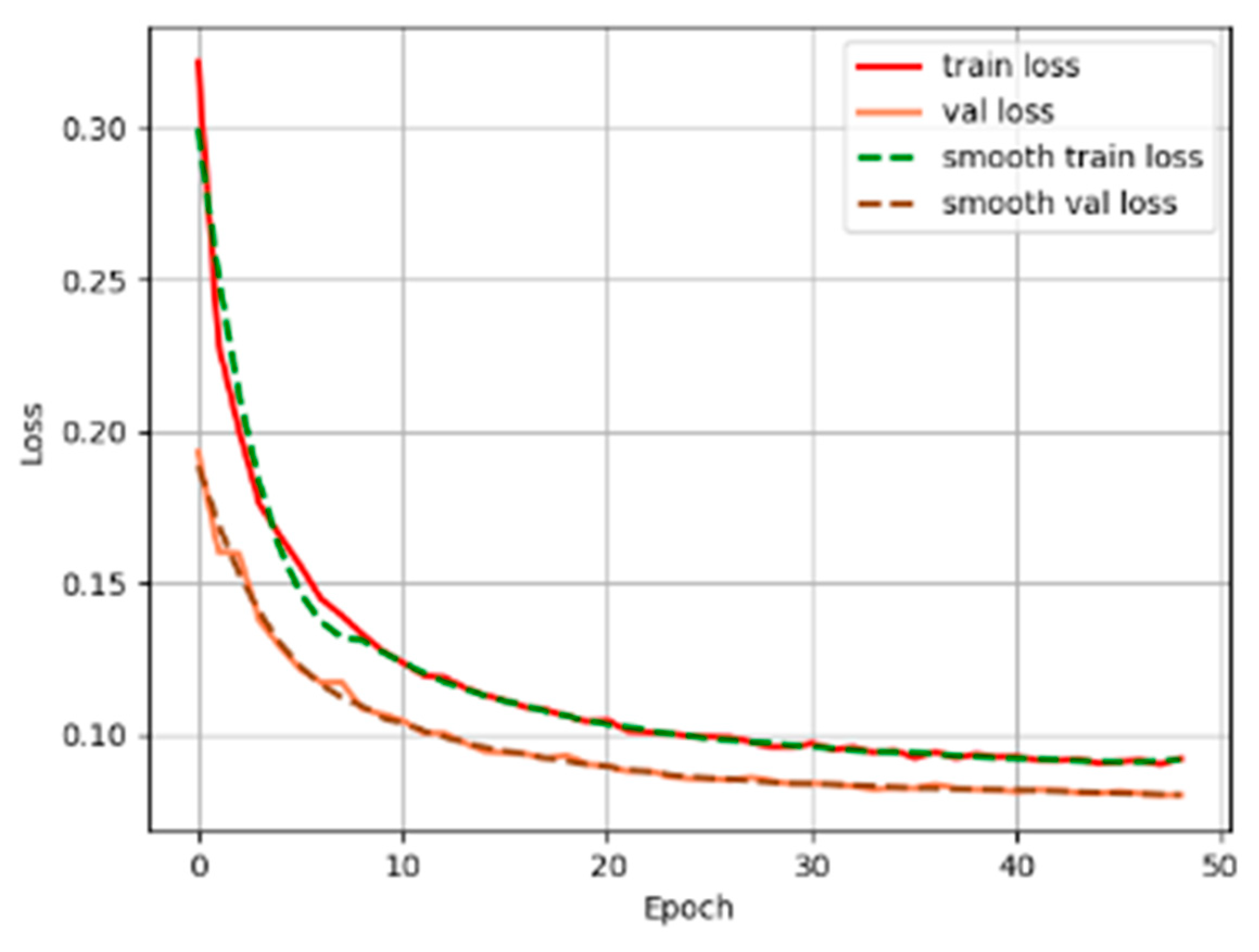
3.3. Training Results of Semantic Segmentation Model

In the experiment, the hyperparameters of the semantic segmentation model were set identical to those in the previous experiment. In the mixed training experiment, convergence was attained around the fortieth epoch, where the training set loss function decreased from 0.307 to 0.111 and the validation set loss function decreased from 0.211 to 0.094. The training graph is depicted below (Figure 12):
In the experiment of training the haze dataset separately, convergence was achieved around the 60th epoch, where the training set loss function decreased from 0.369 to 0.136, and the validation set loss function decreased from 0.444 to 0.111. The training graph is presented below (Figure 13):
In the experiment of training the clear dataset separately, convergence was achieved around the 40th epoch, where the training set loss function decreased from 0.337 to 0.079, and the validation set loss function decreased from 0.192 to 0.049. The training graph is depicted below (Figure 14):
In joint training experiment 1, it is necessary to first train the foggy dataset and then train the clear dataset. The training outcomes of the foggy dataset, trained separately, are utilized as pre-weight inputs into the training process of the clear dataset. The experiment converged around the 30th epoch, where the training set loss function decreased from 0.302 to 0.112, and the validation set loss function decreased from 0.201 to 0.097. The training graph is depicted below (Figure 15):
In joint training experiment 2, it is necessary to first train the clear dataset and then train the foggy dataset. The training outcomes of the clear dataset, trained separately, are utilized as pre-weight inputs into the training process of the foggy dataset. The experiment converged around the 30th epoch, where the training set loss function decreased from 0.113 to 0.085, and the validation set loss function decreased from 0.167 to 0.070. The training graph is depicted below (Figure 16):
Combine the relevant indicators of the above training experiments and summarize them in Table 5:
Except for mixed training, the performance of training the dehazing dataset alone and joint training 2 is superior on the hazy dataset compared to the haze-free dataset, while the performance of training the haze-free dataset alone and joint training 1 is superior on the haze-free dataset compared to the hazy dataset. This phenomenon arises due to the sensitivity of the semantic segmentation model to image features, which tends to be more inclined towards the characteristics of the latest training set.
In transfer learning, the training set used for training the dehazing dataset alone and joint training 2 yields better performance on the hazy dataset compared to the haze-free dataset, while the training set used for training the haze-free dataset alone and joint training 1 demonstrates better performance on the haze-free dataset compared to the hazy dataset. This is attributed to the semantic segmentation model’s sensitivity to image features, which tends to be more biased towards the characteristics of the latest training set.

4. Conclusions

This paper presents an all-weather integrated defogging and drivable area detection algorithm based on deep learning, designed to address the challenges of recognizing unstructured roads and achieving clear environmental perception under adverse weather conditions in current autonomous driving systems. The algorithm improves the Lite-Mobilenetv2 feature extraction module and incorporates a pyramid pooling module integrated with an attention mechanism, enhancing the speed and accuracy of feature extraction. Additionally, a defogging preprocessing module suitable for real-time detection is introduced, transforming foggy images into clear ones to improve the precision of drivable area detection.
In the drivable area detection component, the algorithm replaces the DeepLabv3+ module with grouped convolutions and depthwise separable convolutions, significantly reducing the network depth, computational load, and parameter count, which further accelerates detection and prevents overfitting. In the atrous spatial pyramid pooling module, the introduction of an attention mechanism optimizes the encoder’s structure, leading to higher processing efficiency and accuracy. The defogging preprocessing module uses a physics-based defogging algorithm that enhances the traditional Dark Channel Prior method by adding weighted aggregation-guided filtering and quadtree search for atmospheric light values. This improvement effectively mitigates halo effects and exposure issues at the image edges while enhancing image detail.
The experimental phase employs a transfer learning-based training method, constructing an all-road-condition semantic segmentation model by training on four datasets containing structured and unstructured roads, with and without fog. This strategy not only reduces computational burden but also significantly improves detection accuracy. Experimental results show that the proposed algorithm increases detection efficiency by 3.84% compared to existing algorithms.
Future research will integrate sensor technology to further improve drivable area recognition, optimize the algorithm for processing video data, and enable automatic switching between foggy and non-foggy modes, thereby better adapting to real-world application scenarios.

Author Contributions

Methodology, C.L.; Validation, Q.W.; Formal analysis, Q.W.; Investigation, Q.W.; Resources, C.L.; Writing—original draft, Q.W.; Writing—review & editing, C.L.; Visualization, C.L.; Supervision, Y.L.; Project administration, Y.L.; Funding acquisition, Y.L. All authors have read and agreed to the published version of the manuscript.

Funding

Supported by Science and Technology Department of Sichuan Province No. 2023YFG0317.

Institutional Review Board Statement

Not applicable.

Informed Consent Statement

Not applicable.

Data Availability Statement

The data presented in this study are available in article.

Conflicts of Interest

The authors declare no conflict of interest.

References

  1. Clements, L.M.; Kockelman, K.M. Economic effects of automated vehicles. Transp. Res. Rec. 2017, 2606, 106–114. [Google Scholar] [CrossRef]
  2. Kim, K.; Kim, B.; Lee, K.; Ko, B.; Yi, K. Design of integrated risk management-based dynamic driving control of automated vehicles. IEEE Intell. Transp. Syst. Mag. 2017, 9, 57–73. [Google Scholar] [CrossRef]
  3. Yenikaya, S.; Yenikaya, G.; Düven, E. Keeping the vehicle on the road: A survey on on-road lane detection systems. ACM Comput. Surv. (CSUR) 2013, 46, 1–43. [Google Scholar] [CrossRef]
  4. Almalioglu, Y.; Turan, M.; Trigoni, N.; Markham, A. Deep learning-based robust positioning for all-weather autonomous driving. Nat. Mach. Intell. 2022, 4, 749–760. [Google Scholar] [CrossRef]
  5. Lee, D.-G. Fast Drivable Areas Estimation with Multi-Task Learning for Real-Time Autonomous Driving Assistant. Appl. Sci. 2021, 11, 10713. [Google Scholar] [CrossRef]
  6. Shang, E.; An, X.; Li, J.; Ye, L.; He, H. Robust unstructured road detection: The importance of contextual information. Int. J. Adv. Robot. Syst. 2013, 10, 179. [Google Scholar] [CrossRef]
  7. LeCun, Y.; Bengio, Y.; Hinton, G. Deep Learning. Nature 2015, 521, 436–444. [Google Scholar] [CrossRef] [PubMed]
  8. Zhao, H.; Shi, J.; Qi, X.; Wang, X.; Jia, J. Pyramid scene parsing network. In Proceedings of the 2017 IEEE Conference on Computer Vision and Pattern Recognition, Honolulu, HI, USA, 21–26 July 2017. [Google Scholar]
  9. Zhou, Z.; Siddiquee, M.M.R.; Tajbakhsh, N.; Liang, J. UNet++: A nested U-Net architecture for medical image segmentation. In Proceedings of the Deep Learning in Medical Image Analysis and Multimodal Learning for Clinical Decision Support: 4th International Workshop, DLMIA 2018, and 8th International Workshop, ML-CDS 2018, Held in Conjunction with MICCAI 2018, Granada, Spain, 20 September 2018. [Google Scholar]
  10. Wang, X.; Hu, Z.; Shi, S.; Hou, M.; Xu, L.; Zhang, X. A deep learning method for optimizing semantic segmentation accuracy of remote sensing images based on improved UNet. Sci. Rep. 2023, 13, 7600. [Google Scholar] [CrossRef]
  11. Wang, Y.; Wang, C.; Wu, H.; Chen, P. An improved Deeplabv3+ semantic segmentation algorithm with multiple loss constraints. PLoS ONE 2022, 17, e0261582. [Google Scholar] [CrossRef]
  12. Liu, S.; Li, Y.; Li, H.; Wang, B.; Wu, Y.; Zhang, Z. Visual Image Dehazing Using Polarimetric Atmospheric Light Estimation. Appl. Sci. 2023, 13, 10909. [Google Scholar] [CrossRef]
  13. Wang, C.; Ding, M.; Zhang, Y.; Wang, L. A Single Image Enhancement Technique Using Dark Channel Prior. Appl. Sci. 2021, 11, 2712. [Google Scholar] [CrossRef]
  14. Yan, B.; Yang, Z.; Sun, H.; Wang, C. ADE-CycleGAN: A Detail Enhanced Image Dehazing CycleGAN Network. Sensors 2023, 23, 3294. [Google Scholar] [CrossRef] [PubMed]
  15. Engin, D.; Genc, A.; Ekenel, H.K. Cycle-Dehaze: Enhanced CycleGAN for Single Image Dehazing. In Proceedings of the 2018 IEEE/CVF Conference on Computer Vision and Pattern Recognition Workshops (CVPRW), Salt Lake City, UT, USA, 18–23 June 2018. [Google Scholar]
  16. Li, A.; Xu, G.; Yue, W.; Xu, C.; Gong, C.; Cao, J. Object Detection in Hazy Environments, Based on an All-in-One Dehazing Network and the YOLOv5 Algorithm. Electronics 2024, 13, 1862. [Google Scholar] [CrossRef]
  17. Yu, Y.; Lu, Y.; Wang, P.; Han, Y.; Xu, T.; Li, J. Drivable Area Detection in Unstructured Environments based on Lightweight Convolutional Neural Network for Autonomous Driving Car. Appl. Sci. 2023, 13, 9801. [Google Scholar] [CrossRef]
  18. Chollet, F. Xception: Deep Learning with Depthwise Separable Convolutions. In Proceedings of the 2017 IEEE Conference on Computer Vision and Pattern Recognition (CVPR), Honolulu, HI, USA, 21–26 July 2017; pp. 1800–1807. [Google Scholar] [CrossRef]
  19. Sci, J.H. Relu Deep Neural Networks and Linear Finite Elements. J. Comput. Math. 2020, 38, 502–527. [Google Scholar] [CrossRef]
  20. Song, L.; Fan, J.; Chen, D.R.; Zhou, D.X. Correction: Approximation of Nonlinear Functionals Using Deep ReLU Networks. J. Fourier Anal. Appl. 2023, 29, 57. [Google Scholar] [CrossRef]
  21. Wang, Y.; Li, Y.; Song, Y.; Rong, X. The Influence of the Activation Function in a Convolution Neural Network Model of Facial Expression Recognition. Appl. Sci. 2020, 10, 1897. [Google Scholar] [CrossRef]
  22. Yu, M.; Zhang, W.; Chen, X.; Liu, Y.; Niu, J. An End-to-End Atrous Spatial Pyramid Pooling and Skip-Connections Generative Adversarial Segmentation Network for Building Extraction from High-Resolution Aerial Images. Appl. Sci. 2022, 12, 5151. [Google Scholar] [CrossRef]
  23. Zhu, T.; Liu, Q.; Zhang, L. An Adaptive Atrous Spatial Pyramid Pooling Network for Hyperspectral Classification. Electronics 2023, 12, 5013. [Google Scholar] [CrossRef]
  24. Kardakis, S.; Perikos, I.; Grivokostopoulou, F.; Hatzilygeroudis, I. Examining Attention Mechanisms in Deep Learning Models for Sentiment Analysis. Appl. Sci. 2021, 11, 3883. [Google Scholar] [CrossRef]
  25. An, W.; Wu, G. Hybrid Spatial-Channel Attention Mechanism for Cross-Age Face Recognition. Electronics 2024, 13, 1257. [Google Scholar] [CrossRef]
  26. Liu, B.; Lv, Y.; Gu, Y.; Lv, W. Implementation of a Lightweight Semantic Segmentation Algorithm in Road Obstacle Detection. Sensors 2020, 20, 7089. [Google Scholar] [CrossRef] [PubMed]
  27. Banerjee, S.; Chaudhuri, S.S. Nighttime image-dehazing: A review and quantitative benchmarking. Arch. Comput. Methods Eng. 2021, 28, 2943–2975. [Google Scholar] [CrossRef]
  28. Tsai, C.-Y.; Chen, C.-L. Attention-Gate-Based Model with Inception-like Block for Single-Image Dehazing. Appl. Sci. 2022, 12, 6725. [Google Scholar] [CrossRef]
  29. Zhu, Z.; Luo, Y.; Wei, H.; Li, Y.; Qi, G.; Mazur, N.; Li, Y.; Li, P. Atmospheric light estimation based remote sensing image dehazing. Remote Sens. 2021, 13, 2432. [Google Scholar] [CrossRef]
  30. Wu, L.; Chen, J.; Chen, S.; Yang, X.; Xu, L.; Zhang, Y.; Zhang, J. Hybrid Dark Channel Prior for Image Dehazing Based on Transmittance Estimation by Variant Genetic Algorithm. Appl. Sci. 2023, 13, 4825. [Google Scholar] [CrossRef]
  31. He, K.; Sun, J.; Tang, X. Single image haze removal using dark channel prior. IEEE Trans. Pattern Anal. Mach. Intell. 2010, 33, 2341. [Google Scholar]
  32. Li, C.; Yuan, C.; Pan, H.; Yang, Y.; Wang, Z.; Zhou, H.; Xiong, H. Single-Image Dehazing Based on Improved Bright Channel Prior and Dark Channel Prior. Electronics 2023, 12, 299. [Google Scholar] [CrossRef]
  33. Agrawal, S.C.; Jalal, A.S. A Comprehensive Review on Analysis and Implementation of Recent Image Dehazing Methods. Arch. Comput. Methods Eng. 2022, 29, 4799–4850. [Google Scholar] [CrossRef]
  34. Li, Z.; Zheng, J.; Zhu, Z.; Yao, W.; Wu, S. Weighted Guided Image Filtering. IEEE Trans. Image Process. 2015, 24, 120–129. [Google Scholar]
  35. Chen, B.; Wu, S. Weighted aggregation for guided image filtering. Signal Image Video Process. 2020, 14, 491–498. [Google Scholar] [CrossRef]
  36. Liu, S.; Li, H.; Zhao, J.; Liu, J.; Zhu, Y.; Zhang, Z. Atmospheric Light Estimation Using Polarization Degree Gradient for Image Dehazing. Sensors 2024, 24, 3137. [Google Scholar] [CrossRef] [PubMed]
  37. Haouassi, S.; Wu, D. Image Dehazing Based on (CMTnet) Cascaded Multi-scale Convolutional Neural Networks and Efficient Light Estimation Algorithm. Appl. Sci. 2020, 10, 1190. [Google Scholar] [CrossRef]
  38. Zhu, Z.; Wei, H.; Hu, G.; Li, Y.; Qi, G.; Mazur, N. Novel Fast Single Image Dehazing Algorithm Based on Artificial Multiexposure Image Fusion. IEEE Trans. Instrum. Meas. 2021, 70, 5001523. [Google Scholar] [CrossRef]
  39. Namyup, K.; Dongwon, K.; Cuiling, L. ReSTR: Convolution-free Referring Image Segmentation Using Transformers. IEEE Trans. Circuits Syst. Video Technol. 2018, 28, 3174–3182. [Google Scholar]
  40. Chen, L.C.; Zhu, Y.; Papandreou, G.; Schroff, F.; Adam, H. Encoder-decoder with atrous separable convolution for semantic image segmentation. Comput. Vis. 2018, 833, 801–818. [Google Scholar]
Figure 1. Diagram of the all-weather integrated defogging drivable area detection algorithm process.
Applsci 14 08019 g001
Figure 2. The algorithmic workflow of the feature extraction module.
Applsci 14 08019 g002
Figure 3. Decoder network algorithm.
Applsci 14 08019 g003
Figure 4. Dehazing preprocessing operation flowchart.
Applsci 14 08019 g004
Figure 5. Quadtree search algorithm for atmospheric light value flowchart.
Applsci 14 08019 g005
Figure 6. Quadtree illustration.
Applsci 14 08019 g006
Figure 7. Illustration of the second quadtree operation.
Applsci 14 08019 g007
Figure 8. Illustration of image fusion effect. (a) Original dehazed image; (b) dehazed image after image fusion.
Applsci 14 08019 g008
Figure 9. Comparison of experimental results in simple scenes.
Applsci 14 08019 g009aApplsci 14 08019 g009b
Figure 10. Comparison of experimental results in complex scenes.
Applsci 14 08019 g010
Figure 11. Comparison of dehazing detection experimental results. (a) Clear image; (b) hazy image; (c) detection result of hazy image; (d) detection result of clear image; (e) detection result of hazy image using Cycle-GAN; (f) detection result of hazy image using Dark Channel Prior; (g) detection result of hazy image using AOD-Net; (h) detection result of hazy image using the proposed method.
Applsci 14 08019 g011aApplsci 14 08019 g011b
Figure 12. Mixed training experiment.
Applsci 14 08019 g012
Figure 13. Foggy dataset training experiment.
Applsci 14 08019 g013
Figure 14. Clear dataset training experiment.
Applsci 14 08019 g014
Figure 15. Joint training experiment 1. (a) Previous fog data set training experiment; (b) clear dataset training experiment with pre-trained weights from dehazing dataset.
Applsci 14 08019 g015aApplsci 14 08019 g015b
Figure 16. Joint training experiment 2. (a) Previous training experiment on clear dataset; (b) training experiment on dehazed dataset with pretrained clear weights.
Applsci 14 08019 g016aApplsci 14 08019 g016b
Table 1. Components of the proposed feature extraction module.
Input Size
(H2 × C)
Operatorcns
5122 × 3Conv2d3212
2562 × 32Lite-bottleneck1611
2562 × 16Lite-bottleneck2422
1282 × 24Lite-bottleneck3232
642 × 32Lite-bottleneck6442
322 × 64Lite-bottleneck9631
322 × 96Lite-bottleneck16032
322 × 160Lite-bottleneck32011
Table 2. Training plan.
Training PlanFirst TrainingSecond Training
1Mixed training with dehazed and haze-free datasets
2Dehazed datasetHaze-free dataset
3Haze-free datasetDehazed dataset
4Dehazed dataset
5Haze-free dataset
Table 3. Comparison of network model performance.
ModelmIoU (%)FPS
DeepLabv3+9235.3
U-Net93.612.4
PSP-Net87.8452.6
Proposed Algorithm94.5439.4
Table 4. Comparison of different dehazing algorithm experimental results.
Image CategoriesmIoU (%)Runtime (s)
Hazy image75.02
Clear image94.54
Cycle-GAN87.040.8 (CUDA)
Dark Channel Prior88.430.04
AOD-Net85.590.03 (CUDA)
Proposed method91.550.008 (CUDA)
Table 5. Experimental results.
mIoU (%) on Hazed DatasetmIoU (%) on Clear DatasetAverage mIoU (%)
Mixed training92.3493.3992.865
Training the dehazing dataset separately93.5687.5290.54
Training the haze-free dataset separately91.5594.5493.045
Joint training 191.0291.4391.225
Joint training 294.594.2694.38
Disclaimer/Publisher’s Note: The statements, opinions and data contained in all publications are solely those of the individual author(s) and contributor(s) and not of MDPI and/or the editor(s). MDPI and/or the editor(s) disclaim responsibility for any injury to people or property resulting from any ideas, methods, instructions or products referred to in the content.

