A Path Planning Method Based on Hybrid Sand Cat Swarm Optimization Algorithm of Green Multimodal Transportation

Abstract

Aiming at the difficulty of measuring various costs and time-consuming elements in multimodal transport, this paper constructs a green vehicle comprehensive multimodal transport model which incorporates transportation, transit, quality damage, fuel consumption, and carbon emission costs and proposes a hybrid embedded time window to calculate the time penalty cost in order to reflect the actual transport characteristics. Furthermore, in order to better solve the model, a hybrid sand cat swarm optimization (HSCSO) algorithm is proposed by introducing Logistic–Tent chaotic mapping and an adaptive lens opposition-based learning strategy to enhance the global search capability, and inspired by the swarm intelligence scheme, a momentum–bellicose strategy and an equilibrium crossover pool are introduced to improve the search efficiency and convergence ability. Through testing nine benchmark functions, the HSCSO algorithm exhibits superior convergence accuracy and speed in dealing with complex multi-dimensional problems. Based on the excellent global performance, the HSCSO algorithm was utilized for multimodal vehicle transportation in East China, and a path with a lower comprehensive cost was successfully planned, which proved the effectiveness of the HSCSO algorithm in green intermodal transport path planning.

1. Introduction

As an important part of modern logistics, multimodal transportation integrates different modes of transportation (such as roads, railways, and waterways), improves transport efficiency, and reduces transport costs. The Freight Federation of Europe (FFE) has formulated a series of green standards to encourage enterprises to practice the brand-new concept of green logistics [1]. And, the Japanese government is active in promoting the shift in the mode of trunk transport to foster a new logistical system that meets the requirement on environmental preservation. With the goal set to peak carbon dioxide emissions and achieve carbon neutrality, as well as the improvement of social awareness of a low-carbon environment, green logistics has attracted extensive attention for the development of the logistics industry [2].

Globally, multimodal transportation is studied mainly from two perspectives: cost modeling and path optimization. The research of cost modeling focuses mainly on the costs of transportation and transit involved in the logistical process, customer time window restrictions, and the carbon emissions caused by different modes of transportation. Recent studies on cost modeling in logistics process include: Laurent, A. B. et al. [3], who quantified carbon emissions from the perspective of cost, taking into account transportation costs and delay costs, and established a multi-objective multimodal transport path optimization model that considers carbon emissions. Consider the uncertainty of the transportation environment, that is whether the time, demand, cost, and other factors in the transportation process are certain; Liu, S. [4] considered the time-varying nature of vehicle speed and the time window limit from customers, analyzed the carbon emissions from a multimodal transport system that is affected by the energy consumption of transport vehicles in the time-varying network, and established a model of route optimization for cold chain container multimodal transportation. Bazaluk, O. et al. [5] considered the application of entropy in multimodal transport optimization and prediction, determining risk conditions through deterministic, stochastic, and fuzzy quantities, allowing one to change transport routes in an optimal way in real time and add an unacceptable level of risk to the next phase. Hu, Z. A. et al. [6] aimed at the multimodal transport problem with a mixed uncertain transportation time and demand, based on the comprehensive consideration of the fixed departure time of the transportation mode and the mixed time window composed of the node operation time window and the terminal receipt time window, and adopted the scenario-based robust optimization method to solve the problem.

While these studies have made valuable contributions, most scholars have only focused on the overall delivery time window for the intermodal transportation time window problem, neglecting the time windows during the transportation process. As a result, this paper introduces a new green vehicle comprehensive intermodal transport model, where six aspects of costs are considered and a road congestion index and a hybrid embedded time window are introduced. Our proposed model not only measures transportation costs, carbon emissions, and the transportation time, but also considers the time windows for loading/unloading and the timetables of different transportation modes to better fit the intermodal transportation scenario.

The research of path optimization focuses on the design and improvement of optimization algorithms. As for multimodal transport path optimization, traditional algorithms can be applied, including an ant colony algorithm [7], particle swarm algorithm [8], simulated annealing algorithm [9], genetic algorithm [10], tabu search algorithm [11], etc. In this respect, Piao, C. et al. [12] proposed an improved ant colony optimization algorithm applicable to vehicle routing for logistics distribution, identified the volatility factor according to the search stage, and took into account the distance between the start point, end point, and each node in the heuristic factor. Leng, K. et al. [13] analyzed the vehicle routing problem of multiple distribution centers based on urban rail transit, proposed a novel Concentration-Immune Algorithm Particle Swarm Optimization (C-IAPSO) based on the respective advantages of C-IA and PSO in vehicle path optimization, combining the concept of the antibody concentration. SteadieSeifi, M. et al. [14] used the adaptive large neighborhood search algorithm (ALNS) to solve the problem of considering the uncertainty of customer demand, introduced the destruction operator and the repair operator, and adopted a new priority strategy to optimize the algorithm to improve the search. Kiani, F. et al. [15] proposed two efficient 3D path planning methods inspired by Incremental Grey Wolf Optimization (I-GWO) and Expanded Grey Wolf Optimization (Ex-GWO), which hunt prey by updating the position of the wolf pack based on the leader wolf or the first three wolves, and used it to determine the optimal path for drones.

The Sand Cat Swarm Optimization (SCSO) algorithm is a novel bio-inspired algorithm proposed by Seyyedabbasi, A. and Kiani, F. [16]. Compared with other intelligent algorithms, the SCSO algorithm has a fast convergence speed, few parameters, and is easy to implement. It has a good performance in various fields including path planning, but it is easily disturbed by local optimal points, resulting in the premature convergence of the algorithm and failure to find the global optimal solution. Consequently, numerous studies have concentrated on improving the SCSO algorithm to attain superior results. Adegboye, O. R. et al. [17] combined Dynamic Pinhole Imaging (DPI) and the Golden Sine (Gold-SA) Algorithm with the existing Sand Cat Swarm Optimization to solve the problem of the algorithm falling into local optima as well as premature and delayed convergence. Kiani, F. et al. [18] integrated the chaos feature of non-recurring locations into the core search process of SCSO and proposed a Chaotic Sand Cat Swarm Optimization algorithm (CSCSO) to improve the global search performance and convergence behavior. Lou, T. et al. [19] introduced a hybrid multi-strategy-based sand cat swarm optimization (HMSCSO) algorithm, which adopted the nonlinear adjustment strategy, introduced the logarithmic weight strategy in the position update, and adopted the alternate selection strategy and the position update formula of Lévy flight to enhance the global performance. Wu, D. et al. [20] introduced the wandering strategy including the triangle walk strategy and levy flight walk strategy into the SCSO algorithm, and proposed a Modified Sand Cat Swarm Optimization (MSCSO) Algorithm, which successfully improved the mobility of the sand cat and the global exploration capability of the algorithm.

While existing research efforts aimed at enhancing the SCSO algorithm often concentrate on optimizing the global performance, as mentioned earlier, they frequently overlook the optimization of the sand cat population and the specific process of sand cat search and attack. In this paper, we propose a Hybrid Sand Cat Swarm Optimization (HSCSO) algorithm, which includes Logistic–Tent chaotic mapping and an adaptive lens opposition-based learning strategy, to optimize the initial sand cat population and improve the global performance of the algorithm, and inspired by the swarm intelligence scheme, an inertia–momentum strategy and an elite crossover pool are introduced in the search and attack phases to improve the search efficiency and convergence ability.

The contributions of this work can be summarized as follows. (1) The proposal of the multimodal transport model: considering six aspects including transportation, transfer, quality damage, fuel consumption, carbon emissions, and time penalty costs, and introducing a road congestion index and a hybrid embedded time window, a green vehicle comprehensive multimodal transport model is constructed to better reflect the actual cost situation of multimodal transportation. (2) The improvement of the SCSO algorithm: The initial sand cats are optimized through Logistic–Tent chaotic mapping, and inspired by the swarm intelligence scheme, a momentum–bellicose strategy and an elite crossover pool are introduced to enhance the search performance. Moreover, an adaptive lens opposition-based learning strategy is introduced to enhance the global search capability. The test results indicated that the proposed algorithm is a powerful and effective approach for high-dimension complex optimization. (3) Taking vehicle logistics in east China as an example, the proposed method is successfully applied to multimodal transportation path planning, achieving a reduction in comprehensive costs. The effectiveness of the proposed method in green multimodal transportation path planning has been demonstrated.

The remainder of this paper is structured as follows. In Section 2, the process of building this green vehicle comprehensive multimodal transport model is introduced. In Section 3, the basic sand cat swarm algorithm is introduced. In Section 4, the improved method of the HSCSO algorithm is described in detail. In Section 5, the algorithm is tested against the benchmark function. In Section 6, the proposed model and algorithm are applied to solve the practical multimodal vehicle transportation, and the results are briefly analyzed. In Section 7, the paper concludes with a summary.

2. Green Vehicle Comprehensive Multimodal Transport Model

Considering the green logistics principles of resource conservation and emission reduction, along with the principle of systematicity which supports long-term positive environmental impacts, including route optimization, the cost–environmental impact balance, and optimal transit arrangements, this paper divides the cost generated in transportation into six parts, adopts three transportation modes, Roads, Railways, and Waterways, and builds a specific model as follows.

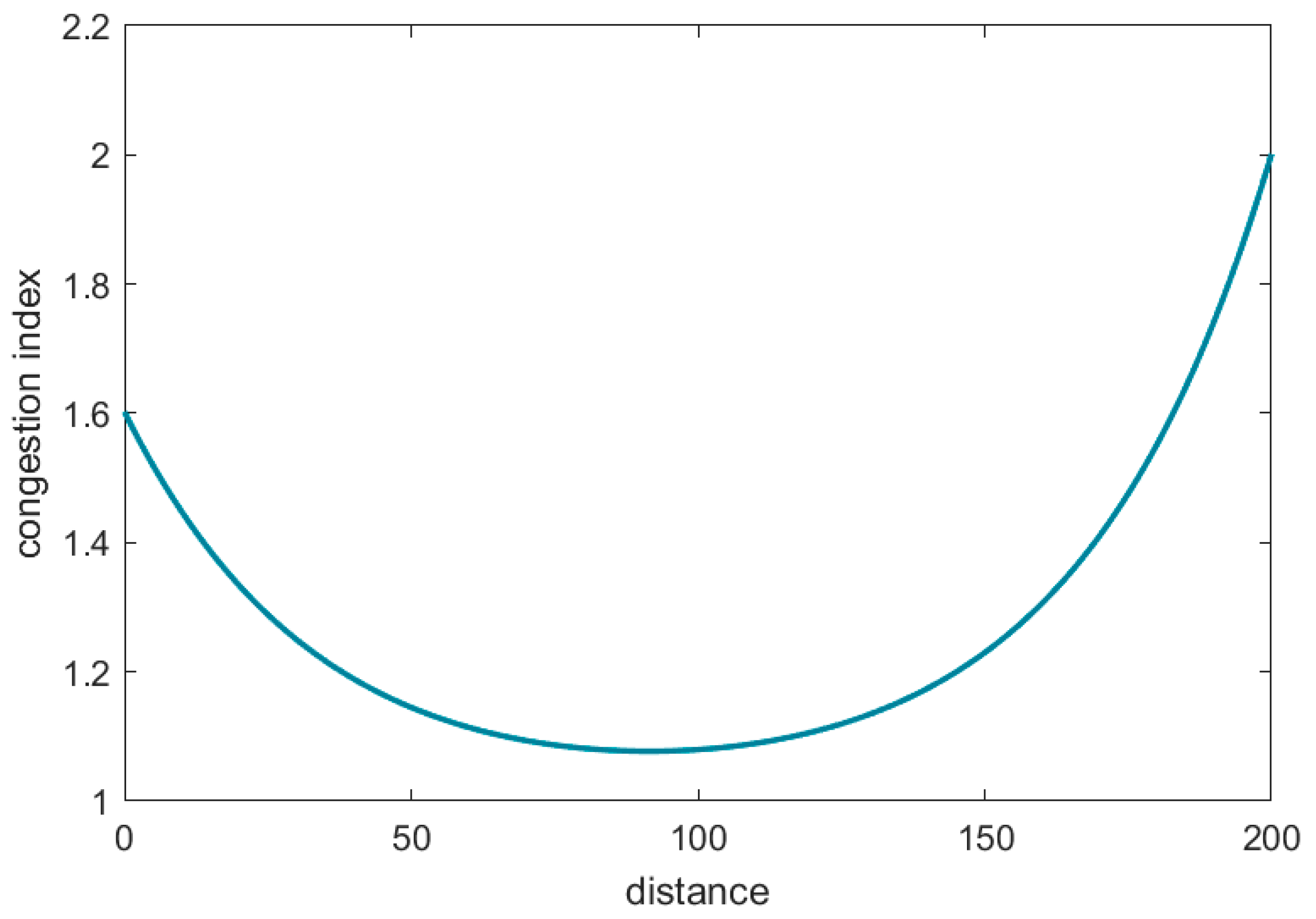
2.1. Road Congestion Index

The road congestion index is usually used to measure the congestion level [21], which is the ratio of the actual travel time to the unblocked travel time [22]. Considering that congestion tends to be more pronounced around transportation hubs, that is, the transfer centers, and the congestion within roads connecting two cities can be considered to be radiated by the congestion surrounding the transfer centers, this radiation attenuates with distance. The congestion index of the road network around each city’s transfer center is queried by Amap (v15.00.0.2031), and this attenuation can be described by an exponential function. Therefore, the congestion index at any point from location i to location j can be described as:

$${Cg}_{ij}^k\left(x\right)=\left({Cg}_i-{Cg}_0\right)e^{-\omega x}+\left({Cg}_j-{Cg}_0\right)e^{-\omega (S_{ij}^k-x)}+{Cg}_0$$

(1)

where ${Cg}_i$ and ${Cg}_j$ represent the congestion index of the road network surrounding the transfer centers in cities i and j, ${Cg}_0$ represents the unblocked congestion index, $\omega$ is the congestion attenuation coefficient, $S_{ij}^k$ refers to the distance from i to j under the mode k of transportation, and x represents any position within the road, the value is from 0 to $S_{ij}^k$. An example of the congestion index for the entire road is shown in Figure 1. By the integral operation, we can describe the average road congestion index ${Cg}_{ij}^k$ and the transportation time $t_s$:

$${Cg}_{ij}^k={\int }_0^{S_{ij}^k}{Cg}_{ij}^k\left(x\right)dx/S_{ij}^{k }$$

(2)

$$t_s={\sum }_{h\in H}{\sum }_{i,j\in V}{\sum }_{k\in K}{X}_{ij}^{hk}{S}_{ij}^k{Cg}_{ij}^k/V^k$$

(3)

where $V^k$ is the speed of transportation mode k. Since trains and ships are not affected by congestion, when railways or waterways are used, ${Cg}_{ij}^k$ = 1.

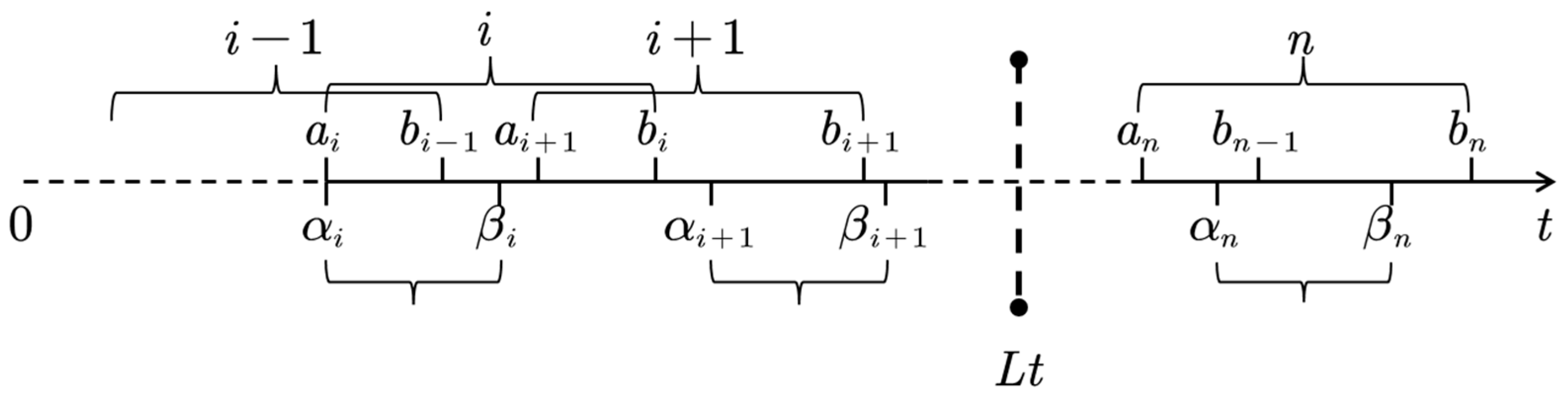
2.2. Hybrid Embedded Time Window

In the current research on transportation issues, the time windows of multimodal transportation almost only include soft or hard time windows for delivery, ignoring that although changing transportation modes can increase transportation flexibility [23], there will be a waiting time due to the loading and unloading of the cargo and the timetables of trains or ships. Aiming at this situation, a hybrid embedded time window is introduced in this paper.

The total delivery time window is a unilateral soft time window, in which cargo delivered later than the threshold time are subject to a certain penalty cost. The penalty cost is in the form of an inverse tangent function to describe the time penalty effect more flexibly and non-linearly, and to avoid transitional penalties by relying on the property of its decreasing rate of change. The setting is as follows:

$$p_1\left(t\right)=\left\{\begin{array}{cc}\hfill 0,& 0<t<Lt\hfill \\ \hfill {\displaystyle \frac{200}{\pi }}arctan(\lambda (t-Lt)),& t\ge Lt\hfill \end{array}\right.$$

(4)

where $\lambda$ represents the time penalty coefficient.

Considering that cargo arriving at the buffer area needs to queue for unloading and trans-shipment due to limited equipment, an arrangement time window is introduced to indicate the availability of loading and unloading equipment. Additionally, a staggered time window group is introduced to indicate the arrival and waiting of trains and ships considering their fixed schedules. Both the arranged and interleaved time windows are combined with the unilateral soft time of delivery and a hybrid embedded time window is obtained, as shown in Figure 2.

Cargo in the buffer area will be fined for the additional buffer burden caused by waiting. The unloading time window groups are defined as ${(a}_i, b_i)$, indicating that cargo arriving within this time frame, with sufficient remaining time to complete unloading, can be processed by the equipment. Otherwise, the cargo must wait until the next time window ${(a}_{i+1}, b_{i+1})$. The waiting time window groups for trains or ships are defined as $({\alpha }_i, {\beta }_i)$, within which cargo that completes unloading can be promptly loaded onto different modes of transportation and depart collectively at time ${\beta }_i$.

Firstly, focusing on the unloading time window, let $t_a$ represent the time the cargo arrives at the buffer area; $t_b^j (j=1, 2)$ represent the waiting time in the j-th time window, typically caused by arriving outside the time window or insufficient remaining time within the current window to complete unloading, leading to loading/unloading delays; $t_u$ denote the time required for unloading, which is related to the handling operations and the quantity of cargo; and $t_c^j$ represent the time of departure from the j-th time window. Thus, we have:

$$t_b^1=\left\{\begin{array}{ll}0,\hfill & t_a+t_u\le b_i\hfill \\ & a_{i+1}-t_a, t_a+t_u>b_i\hfill \end{array}\right.{ t}_c^1=\left\{\begin{array}{c}{t}_a+t_u, t_a+t_u\le b_i\\ a_{i+1}+t_u, t_a+t_u\le b_i\end{array}\right.$$

(5)

Then, the cargo waits to depart by train or ship. Focusing on the docking time window for trains or ships, we have:

$$t_b^2=\left\{\begin{array}{cc}0,& {\alpha }_i<t_c^1<{\beta }_i\hfill \\ & a_{i+1}-t_c, {\beta }_i<t_c^1<{\alpha }_{i+1}\end{array}\right. t_c^2=\left\{\begin{array}{c}{\beta }_i, {\alpha }_i<t_c^1<{\beta }_i\\ {\beta }_{i+1}, {\beta }_i<t_c^1<{\alpha }_{i+1}\end{array}\right.$$

(6)

Let $d^h$ represent the number of complete vehicles which are fully assembled and transported as cargo and let $p_w$ represent the waiting cost per unit of time per complete vehicles as cargo. Let $t_{ts}$ represent the total transit time, which is calculated as $t_c^2-t_a$, and the penalty cost for waiting in the buffer is calculated as:

$$p_2(t_w)=t_w{p}_w{d}^h$$

(7)

2.3. Model Construction

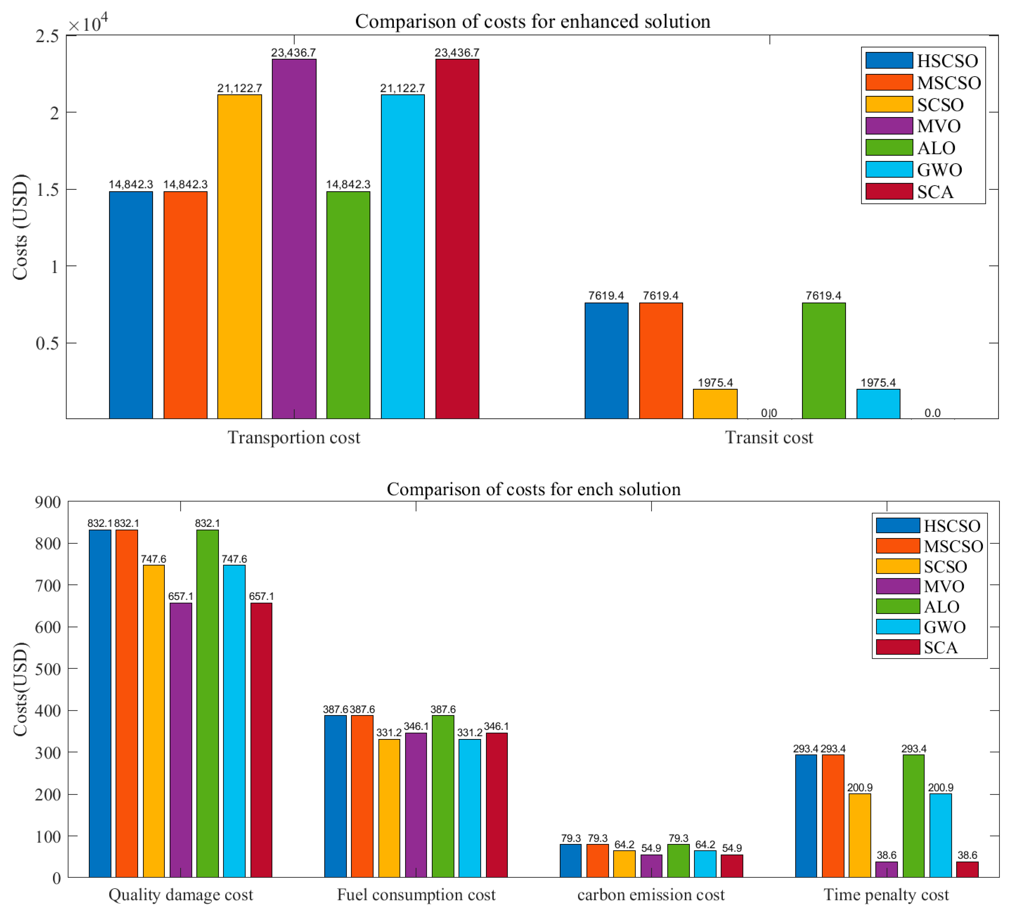
2.3.1. Transportation Cost

The cost of transporting a complete vehicle between two nodes is affected by the prices and transportation distances of different modes of transportation, excluding tolls, service fees, and other miscellaneous expenses, namely:

$$C_1={\sum }_{h\in H}{\sum }_{i,j\in V}{\sum }_{k\in K}{X}_{ij}^{hk}{S}_{ij}^{hk}{Er}_{ij}^k{d}^h$$

(8)

where H represents the set of transported vehicles as cargo; V indicates the set of nodes that can be passed through during transportation; K denotes the set of transportation modes that can be adopted; $S_{ij}^k$ refers to the distance from i to j under mode k of transportation; ${Er}^k$ indicates the distance rate from i to j under mode k of transportation; $d^h$ denotes the number of complete vehicles as cargo; and $X_{ij}^{hk}$ represents the transportation mode decision variable, which means:

$$X_{ij}^{hk}=\left\{\begin{array}{c}1, \mathrm{u}\mathrm{s}\mathrm{i}\mathrm{n}\mathrm{g} \mathrm{t}\mathrm{r}\mathrm{a}\mathrm{n}\mathrm{s}\mathrm{p}\mathrm{o}\mathrm{r}\mathrm{t} \mathrm{m}\mathrm{o}\mathrm{d}\mathrm{e} k \mathrm{f}\mathrm{r}\mathrm{o}\mathrm{m} i \mathrm{t}\mathrm{o} j\\ 0, \mathrm{e}\mathrm{l}\mathrm{s}\mathrm{e}\end{array}\right.$$

(9)

2.3.2. Transit Cost

The transit cost mainly covers the costs incurred by transfer, the loading and unloading of the complete vehicle when the mode of transportation is changed at the node, taking into account the number of complete vehicles and the cost of switching between different modes of transportation, namely:

$$C_2={\sum }_{h\in H}{\sum }_{i\in V}{\sum }_{p,q\in K}{Y}_{hi}^{pq}{Tr}_i^{pq}{d}^h+C_e$$

(10)

where ${Tr}_i^{pq}$ represents the transfer rate, given the change in mode of transportation from p to q at node i, $d^h$ indicates the number of transported complete vehicles as cargo, $C_e$ denotes the cost of short-distance transportation and other surcharges, and $Y_{hi}^{pq}$ refers to the transfer mode decision variable, which means:

$$Y_{hi}^{pq}=\left\{\begin{array}{c}1, \mathrm{c}\mathrm{h}\mathrm{a}\mathrm{n}\mathrm{g}\mathrm{i}\mathrm{n}\mathrm{g} \mathrm{t}\mathrm{r}\mathrm{a}\mathrm{n}\mathrm{s}\mathrm{p}\mathrm{o}\mathrm{r}\mathrm{t} \mathrm{m}\mathrm{o}\mathrm{d}\mathrm{e} \mathrm{f}\mathrm{r}\mathrm{o}\mathrm{m} p \mathrm{t}\mathrm{o} q \mathrm{a}\mathrm{t} i.\\ 0, \mathrm{e}\mathrm{l}\mathrm{s}\mathrm{e}\end{array}\right.$$

(11)

2.3.3. Quality Damage Cost

Consideration is given to the cost of quality damage of the vehicle during transportation, including adverse weather and traffic accidents, as well as possible damage caused during loading and unloading, namely [24]:

$$C_3={\sum }_{h\in H}{\sum }_{i,j\in V}{\sum }_{k\in K}{X}_{ij}^{hk}{p}^h{d}^h\left(1-e^{-Z_k{S}_{ij}^k}\right)+{\sum }_{h\in H}{\sum }_{i\in V}{\sum }_{p,q\in K}{Y}_{hi}^{pq}{p}^h{d}^h\left(1-e^{-Z_{pq}}\right)$$

(12)

where $p^h$ represents the unit price of cargo h, $d^h$ denotes the number of complete vehicles as cargo, $Z_k$ denotes the damage rate of cargo during transportation when mode k of transportation is selected, and $Z_{pq}$ refers to the damage rate of cargo when mode p of transportation is changed to q at the node.

2.3.4. Fuel Consumption Cost

The fuel consumption cost is calculated using the unit fuel price and fuel consumption under each mode of transportation. Let ${Gf}^k$ represent the unit fuel cost incurred under mode k of transportation, and $F_{ij}^{kh}$ is the fuel consumption of cargo h from i to j under mode k of transportation, namely:

$$C_4={\sum }_{h\in H}{\sum }_{i,j\in V}{\sum }_{k\in K}{{Gf}^{k}X}_{ij}^{hk}{F}_{ij}^{kh}$$

(13)

In the case of road transportation, due to the limitation of the carrying capacity, multiple lorries are often needed in one transportation task. The relationship between the fuel consumption and cargo volume cannot be simplified into a direct proportion. $S_{ij}^k$ represents the distance from i to j under mode k of transportation; Q is refers to the capacity of the lorry; $f_1$ and $f_2$ refer to the fuel consumption per unit of distance of the lorry when it is empty and fully loaded, respectively; [25] and $N_{min}^h$ indicates the minimum number of lorries required. $N_{min}^h=⌈{\displaystyle \frac{d^a}{Q}}⌉+⌈{\displaystyle \frac{d^b}{Q}}⌉$, where $d^a$ and $d^b$, respectively, represent the volume of two types of cargo that cannot be mixed, $d^a+d^b=d^h$, and fuel consumption is expressed as follows:

$$F_{ij}^{load}=\left[f_1{N}_{min}^h+d^h\left({f_2-f}_1\right)/Q\right]S_{ij}^k$$

(14)

In the case of railway or waterway transportation, most of the fuel is diesel and the energy consumption coefficient is 0.0025 kg/t·km and 0.0056 kg/t·km, respectively. ${\mu }^k$ represents the energy consumption coefficient under mode k of transportation. Thus,

$$F_{ij}^{r\&w}={{\mu }^k{d}^{h}S}_{ij}^k$$

(15)

2.3.5. Carbon Emission Cost

The carbon emission costs in vehicle logistics mainly cover the carbon emission costs incurred by the fuel consumed during the process of transportation and the transfer, loading, and unloading. The carbon emissions caused by the consumed fuel are calculated using fuel consumption and emission factors, which is the conversion method for energy consumption [26], namely:

$$C_5={\sum }_{h\in H}{\sum }_{i,j\in V}{\sum }_{k\in K}{\delta X}_{ij}^{hk}{F}_{ij}^{kh}D+{\sum }_{h\in H}{\sum }_{i\in V}{\sum }_{p,q\in K}{Y}_{hi}^{pq}{d}^h{\rho }^{pq}D$$

(16)

where $\delta$ represents the carbon emission coefficient of fuel, ${\rho }^{pq}$ indicates the carbon emission coefficient of transportation mode p to q, and D refers to the carbon tax price.

2.3.6. Time Penalty Cost

The time penalty cost is calculated based on the hybrid embedded time window mentioned above, including the late arrival cost of the vehicle failing to reach the demand point before the specified time, and the waiting cost of staying in the cache area, which increases the cache pressure, namely:

$$C_6=p_1\left(\sum t_s+\sum {(t}_d-t_a)\right)+p_2\left(\sum t_b\right)$$

(17)

where $t_s$ represents the transportation time excluding the transit time, ${(t}_d-t_a)$ represents the transit time from entering the buffer zone to completing the conversion of the transportation mode, and $t_b$ refers to the blocking time excluding loading or unloading in the buffer zone.

In summary, the optimization objective function and constraints are as follows:

$$minC=C_1+C_2+C_3+C_4+C_5+C_6$$

(18)

$$s.t.\left\{\begin{array}{c}{X}_{ij}^{hk}\left(X_{ij}^{hk}-1\right)=0, \forall (i,j)\in V,\forall h\in H,\forall k\in K\\ Y_{hi}^{pq}\left(Y_{hi}^{pq}-1\right)=0, \forall i\in V,\forall h\in H,\forall (p,q)\in K\\ X_{ij}^{hp}+X_{jl}^{hq}\ge 2Y_{hj}^{pq}, \forall (i,j)\in V,\forall h\in H,\forall (p,q)\in K\\ {\sum }_{k\in K}{X}_{ij}^{hk}=1\end{array}\right.$$

Among them, Equation (18) is the objective function formula used for minimizing the comprehensive total cost. The first constraint means that only one mode of transportation can be used between two nodes; the second constraint indicates that node i can only be changed into one mode of transportation; the third constraints indicates the uninterrupted transportation of the cargo; and the forth constraints indicates that the mode of transportation cannot be changed in transportation between two nodes.

2.4. Model Assumptions

(1)

The transportation volume cannot be divided. The same batch of vehicles can be transported through the only route. Also, only one mode of transportation can be selected between two nodes, and this mode can be changed only at the node.

(2)

If the transportation mode is not changed when passing through the transfer node, there is no transfer, with no carbon emission costs incurred.

(3)

The process of transportation is in an ideal state, the speed of transport is constant, and the impact of emergencies is negligible, such as extreme weather and traffic accidents.

(4)

Lorries, trains, and ships are single models in their respective categories, each with the same capacity and fuel consumption. The number of vehicles transported in a single trip is smaller than the capacity of railway or waterway transport.

(5)

The short-distance transportation at transfer points and terminal handovers are discounted.

(6)

The weight of the vehicles is constant and the unit price is known.

3. The Sand Cat Swarm Optimization Algorithm

3.1. Initialize Population

In a d dimensional optimization problem, a sand cat is a $1\times d$ array representing the solution to the problem, defined as $Sand Ca{t}_i=[x_1,x_2,\dots ,x_d];i\in \mathrm{p}\mathrm{o}\mathrm{p}\mathrm{u}\mathrm{l}\mathrm{a}\mathrm{t}\mathrm{i}\mathrm{o}\mathrm{n}(1,\mathrm{n})$. Each $x$ must be between the upper and lower bounds: $\forall x_i\in [\mathrm{l}\mathrm{o}\mathrm{w}\mathrm{e}\mathrm{r},\mathrm{u}\mathrm{p}\mathrm{p}\mathrm{e}\mathrm{r}]$. When the SCSO algorithm is used, it first creates an initialization matrix ${(N}_{pop}\times N_d)$ according to the problem size. The fitness cost of each sand cat is obtained by evaluating the defined fitness function. When an iteration is completed, the sand cat with the best cost so far in that iteration is selected. If no better solution is found in the next iteration, it is unnecessary to store it in memory.

3.2. Search for Prey

The SCSO algorithm benefits from the auditory capability of sand cats in low-frequency detection. Sand cats can perceive low frequencies below 2 kHz. In the algorithm, this sensitive range is defined as $r_G$. According to the working principle of the algorithm, this value will linearly decrease from 2 to 0 during the iterative process, gradually approaching the prey without missing or skipping. The $S_m$ simulates the auditory characteristics of the sand cat, with the assumption being 2. The mathematical model is defined as follows:

$$r_G=S_m-({\displaystyle \frac{S_m\times {iter}_c}{{iter}_{Max}}})$$

(19)

where ${iter}_c$ is the current iteration number and ${iter}_{Max}$ is the maximum iteration.

The main parameter controlling the transition is between the exploration phase and the development phase is R. Due to this adaptive strategy, the transition and possibility between the two phases will be more balanced. R is defined as follows:

$$R=2\times r_G\times rand(0,1)-r_G$$

(20)

To avoid falling into local optima, the sensitivity range of each sand cat is different, defined as:

$$r=R\times rand(0,1)$$

(21)

In the SCSO algorithm, the sand cat updates its position based on the optimal solution, its current position, and the sensitivity range, searching for other potential best prey positions. This search behavior can be defined as:

$$Pos(t+1)=r\times \left({Pos}_{bc}\right(t)-rand(0,1)\times {Pos}_c(t\left)\right)$$

(22)

where ${Pos}_{bc}$ is the optimal candidate position and ${\mathrm{P}\mathrm{o}\mathrm{s}}_{\mathrm{c}}$ is the current position.

3.3. Attack Prey

When a sand cat attacks its prey, it first uses the best position ${Pos}_b$ and the current position ${Pos}_c$ to generate a random position ${Pos}_{rnd}$. Assuming that the sensitive range of the sand cat is a circle, to avoid falling into the local optimum, the roulette method is used to randomly select an angle for each sand cat, as shown in Figure 3, so that the sand cat can approach the hunting position:

$${Pos}_{rnd}=\left|rand(0,1)\times {Pos}_b\left(t\right)-{Pos}_c\left(t\right)\right|$$

(23)

$$Pos(t+1)={Pos}_b\left(t\right)-r\times {Pos}_{rnd}\times cos\left(\theta \right)$$

(24)

3.4. Implementation of the SCSO Algorithm

The search and attack phase of the SCSO Algorithm are ensured by adaptive $r_G$ and $R$. These parameters allow SCSO to switch seamlessly between the two phases. When $\left|\mathrm{R}\right|>1$, the sand cats search for prey; when $\left|R\right|\le 1$, the sand cats attack prey. The pseudo-code of the SCSO algorithm is illustrated in Algorithm 1.

Algorithm 1 The framework of SCSO algorithm
1:	Initialize the algorithm-related parameters $S_m$, $r, {\mathrm{r}}_{\mathrm{g}}$, and R
2:	Initialize the maximum generations $G$
3:	Initialize the number of the population $NP$
4:	Initialize the population
5:	Calculate the fitness function based on the objective function
6:	While ($t \le t_{max}$)
7:	For each finder
8:	If $\left(\left|R\right|>1\right)$
9:	The finder conducts searching behavior based on Formal (19)
10:	Else
11:	Randomize the target of attack $\mathrm{P}\mathrm{o}{\mathrm{s}}_{\mathrm{r}}$
12:	The finder conducts attacking behavior based on Formal (19)
13:	end if
14:	end for
15:	t++
16:	end while

4. Hybrid Sand Cat Swarm Optimization Algorithm

The sand cat swarm optimization (SCSO) algorithm [17] is widely employed for real optimization problems due to its rapid convergence, ease of application, and robustness. However, the initial population of the standard SCSO algorithm is randomly generated, and no mutation mechanism is introduced, so its global search ability is relatively weak. In addition, the optimization direction is constantly changing in the process of search and attack, and the local search ability needs to be improved. In this section, we adopted Logistic–Tent chaotic mapping to optimize the initial population and introduced an adaptive lens opposition-based learning strategy to enhance the global search capability. Additionally, drawing inspiration from the swarm intelligence scheme, an inertia–momentum strategy and an elite crossover pool are introduced to improve the search efficiency and convergence ability.

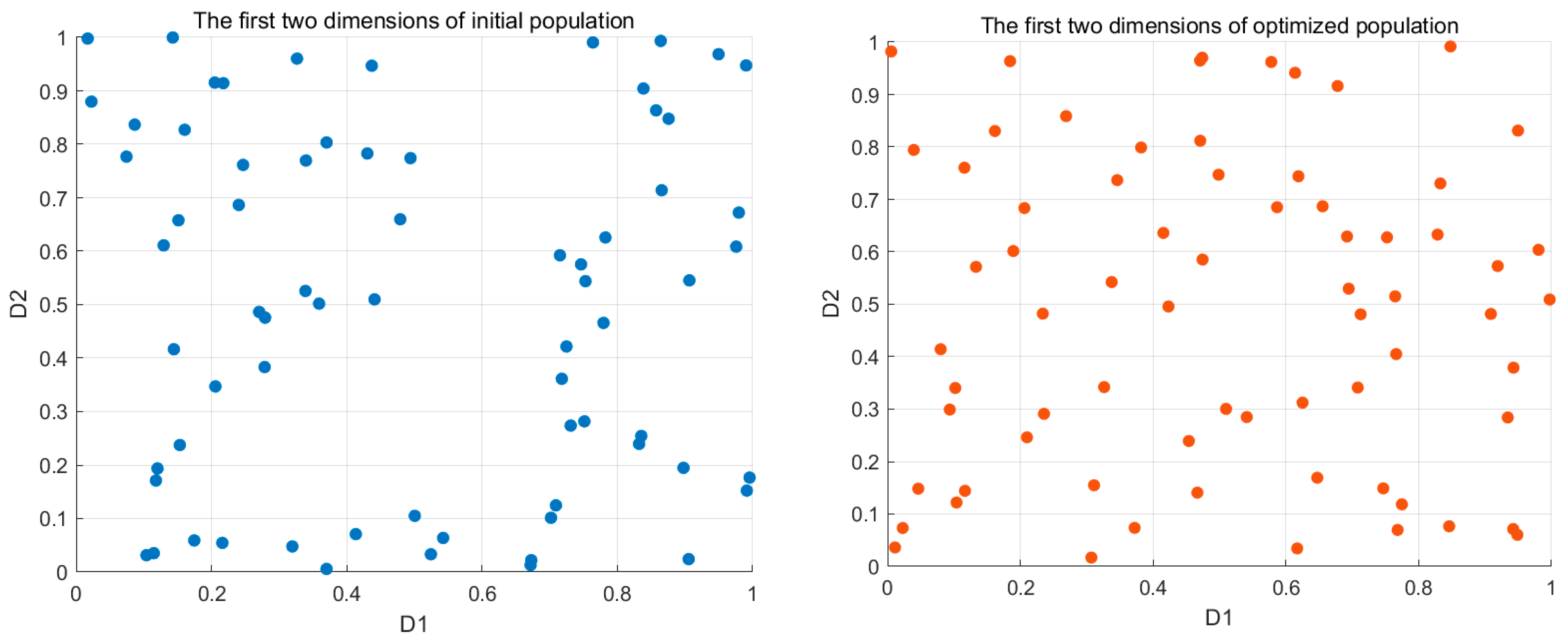
4.1. Logistic–Tent Chaotic Mapping Initialization

In order to improve the efficiency of sand cats conducting a search in the early stage, it is proposed in this paper to generate simulated positions of sand cats through Logistic–Tent chaotic mapping. The randomness and nonlinearity of this mapping can make the initial sand cat population more diverse and random and help the algorithm to explore more widely in the search space and avoid falling into the local optimal solution.

Logistic–Tent chaotic mapping integrates the Logistic and the Tent mapping, which have limited folding times in the iteration region and the existence of rational fixed points, and combines the complex chaotic dynamics of the Logistic mapping and the faster iteration speed and more autocorrelation of the Tent mapping [27]. Its mathematical formula is defined as follows:

$$X_{i+1}=\left\{\begin{array}{c}\left(r{X}_i\right(1-X_i)+(4-r)X_i/2)mod1,X_i<0.5\\ \left(r{X}_i\right(1-X_i)+(4-r\left){(1-X}_i\right)/2)mod1,X_i\ge 0.5\end{array}\right. r\in (0,4)$$

(25)

Figure 4 shows a comparison between the initial and optimized population in the first two and three dimensions, where blue and orange dots represent the original and optimized populations respectively. It can be clearly seen that Logistic–Tent chaotic mapping is used to determine an initial population that is evenly distributed within the space of search. This way of initialization is effective in reducing the probability of local convergence throughout the optimization process.

4.2. Introduction of Momentum–Bellicose Strategy in Search and Attack

When $\left|R\right|>1$, the sand cat relies on the release of low-frequency noise for the prey search. But in the early stage of optimization, the exploration of the search space by the sand cat swarm remains at a preliminary level, the quality of prey is poor and the optimal position of the prey changes frequently. Therefore, if the sand cat relies solely on the location of the optimal prey for search, it can lead to the inconsistent directions of searches and a waste of computing power. In order to enhance the performance of the sand cat swarm in conducting searches at the early stage of optimization, this algorithm introduces a momentum strategy as it allows the sand cat to adjust the search angle progressively under the action of momentum even if the direction of search changes suddenly. Thus, the range of search is widened and the efficiency of search is improved.

$$\overrightarrow{Po{s}_c}\left(t+1\right)=\overrightarrow{r_1}\left(\overrightarrow{Po{s}_b}\left(t\right)-rand\left(0,1\right)\overrightarrow{Po{s}_c}\left(t\right)\right)+c_{1}rand\left(0,1\right)∆\overrightarrow{Po{s}_c}\left(t\right)$$

(26)

$$\overrightarrow{r_1}=\overrightarrow{r_G}rand(0,1)$$

(27)

$$\overrightarrow{r_G}=s_M-{\displaystyle \frac{s_{M}t}{T}}$$

(28)

where $\overrightarrow{Po{s}_c}\left(t+1\right)$ represents the updated position of the sand cat; $\overrightarrow{Po{s}_b}\left(t\right)$ indicates the optimal position of the sand cat; $s_M$ denotes the hearing characteristic parameter of the sand cat; $\mathrm{t}$ is referred to as the current number of iterations; $T$ stands for the maximum number of iterations; $∆\overrightarrow{Po{s}_c}\left(t\right)$ denotes the cumulative momentum of the sand cat; and $c_1$ represents the momentum factor.

When $\left|R\right|\le 1$, the sand cat attacks the prey. In the middle and late stages of the algorithm, the aggressive behavior of the sand cat is performed mainly in the stage of a local search. In order to improve the outcome of a local search by the algorithm, a bellicose factor based on random prey selection is introduced in this paper. This factor prompts the sand cat to move closer to the current optimal position of the sand cat at a certain ratio, thus improving the performance of the algorithm in convergence at the middle and later stages.

$$\overrightarrow{Po{s}_r}\left(t+1\right)=\left|rand\left(0,1\right)\times \overrightarrow{Po{s}_b}\left(t\right)-\overrightarrow{Po{s}_c}\left(t\right)\right|$$

(29)

$$\overrightarrow{Po{s}_c}\left(t+1\right)=\overrightarrow{Po{s}_b}\left(t\right)-\overrightarrow{r_1}\times \overrightarrow{Po{s}_r}\left(t\right)\mathit{cos}\left(\theta \right)+c_2 rand\left(0,1\right)\left(\overrightarrow{Po{s}_b}\left(t\right)-\overrightarrow{Po{s}_c}\left(t\right)\right)$$

(30)

where $\overrightarrow{Po{s}_r}\left(t+1\right)$ represents the random direction chosen by the sand cats when attacking; $\theta$ indicates the random angle; and $c_2$ denotes the bellicose factor.

4.3. Elite Crossover Pool

The elite crossover pool is inspired by the elite strategy [28], for which the idea is to directly share information with some poor performing sand cats from the best prey explored in the search space in order to update the sand cats that have deteriorated under the influence of randomness and enhance the convergence ability of the algorithm in the middle and late stages. After each generation of updates, the positions of the two best performing sand cats and their means are selected as the optimal solution set, and the 10% of individuals with the worst performing sand cats are selected as the crossover objects, which have an equal probability of selecting one of the optimal solutions for crossover, that is:

$$\overrightarrow{Po{s}_{new}}=\overrightarrow{Po{s}_c}\left(t\right)+0.5rand\left(0,1\right)\times \left(\overrightarrow{Po{s}_b}\left(t\right)-\overrightarrow{Po{s}_c}\left(t\right)\right)$$

(31)

Most inferior solutions will be greatly improved through the elite crossover pool, and the local search ability of the algorithm will be enhanced. To cope with the situation of worsening after an update, the Metropolis acceptance criterion is introduced. For each individual after the update and crossover, whether to accept the restoration is evaluated. If the probability does not meet the acceptance condition, the evolution of the sand cat in this generation is canceled. The probability p of acceptance is:

$$p=\left\{\begin{array}{c}1, if y_{new}<y_{old} \\ exp(-\left(y_{new}-y_{old}\right)/t_{iter}), if y_{new}\ge y_{old} \end{array}\right.$$

(32)

where $y_{old}$ and $y_{new}$ are the values before and after the update of the sand cat, respectively, and $t_{iter}$ represents the parameter that decreases with the number of outer loops.

4.4. Adaptive Lens Opposition-Based Learning Strategy for Mutation

The traditional SCSO algorithm does not involve mutation and the search process depends largely on the search range obtained during initialization. Therefore, the adaptive lens opposition-based learning strategy [29] is adopted instead of a general mutation in this paper, which can generate a reverse position for sand cat individuals through a hypothetical lens in the middle of the search space. The individual continues to explore in this reverse position, thereby expanding the search range and enhancing the global performance of the algorithm. According to the principle of lens imaging, the formula is:

$$\overrightarrow{Po{s}_{new}}={\displaystyle \frac{ul+bl}{2}}+{\displaystyle \frac{ul+bl}{2k}}+{\displaystyle \frac{\overrightarrow{Po{s}_c}}{k}}$$

(33)

where ul and bl represent the upper and lower limits of the solution space and k represents the focal length of the lens. A bigger k generates a smaller range of reverse solutions. Combined with the need for taking a larger disturbance amplitude for the population with poor fitness to increase the global search ability of the algorithm, an adaptive k is introduced:

$$k={\displaystyle \frac{y_{max}\left(X\right)-y\left(X\right)}{{\left(y_{max}\left(X\right)-y_{min}\left(X\right)\right)}^2}}$$

(34)

where $y_{max}\left(X\right)$ and $y_{min}\left(X\right)$ represent the current iteration and the maximum and minimum fitness values in the population.

The pseudo-code of the HSCSO algorithm is illustrated in Algorithm 2.

Algorithm 2 The framework of HSCSO algorithm
1:	Initialize the algorithm-related parameters $S_m$$, r,{\mathrm{r}}_{\mathrm{g}}$, and R
2:	Initialize the maximum generations $G$
3:	Initialize the number of the population $NP$
4:	Initialize population using Logistic–Tent chaotic mapping by Formula (18)
5:	Calculate the fitness function based on the objective function
6:	While ($t \le t_{max}$)
7:	For each finder
8:	If $\left(\left|R\right|>1\right)$
9:	The finder conducts searching behavior
10:	Update the finder’s position with the momentum strategy using Formal (19)
11:	Else
12:	The finder conducts attacking behavior
13:	Randomize the target of attack $\mathrm{P}\mathrm{o}{\mathrm{s}}_{\mathrm{r}}$
14:	Update the finder’s position with the bellicose factor using Formal (23)
15:	end if
16:	Add the two best finder positions and their means to the elite crossover pool
17:	For 10% worst finder
18:	Randomly crossover with a solution from the elite crossover pool using Formal (24)
19:	end for
20:	Conduct the adaptive lens opposition-based learning according to Formula (26)
21:	t++
22:	end while

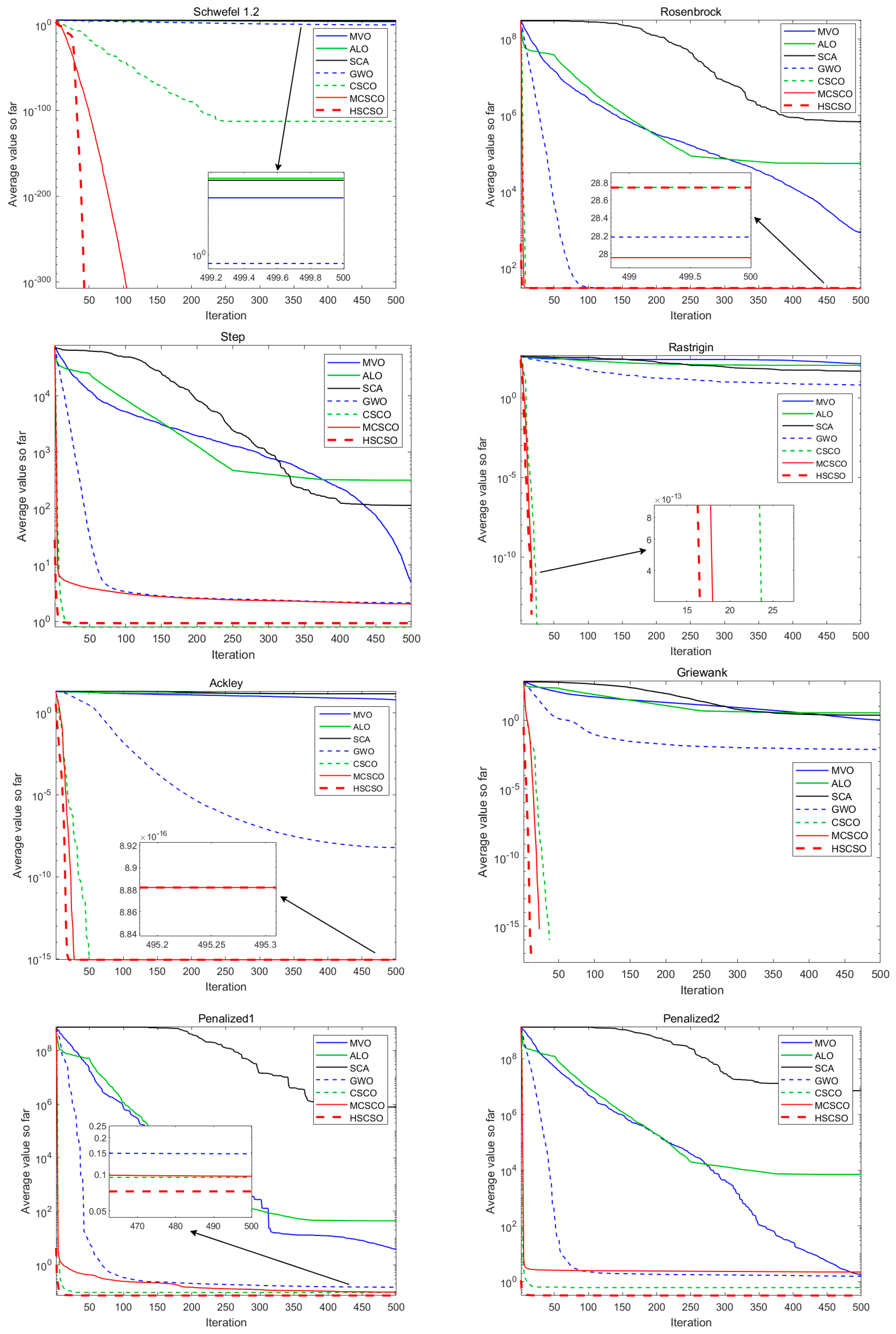
5. Experiment for Benchmark Functions

The CEC2014 benchmark function is used for comparing the performance of different algorithms on a unified standard in this section and the ten typical benchmark functions listed in

Table 1. Ten benchmark functions.

Name	Definition	Domain	Minimum
Sphere	${\mathrm{F}}_1\left(\mathrm{x}\right)=\sum _{\mathrm{i}=1}^{\mathrm{n}}{\mathrm{x}}_{\mathrm{i}}^2$	[−100, 100]	0
Schwefel 2.22	${\mathrm{F}}_2\left(\mathrm{x}\right)=\sum _{\mathrm{i}=1}^{\mathrm{n}}\left|{\mathrm{x}}_{\mathrm{i}}\right|+\prod _{\mathrm{i}=1}^{\mathrm{n}}\left|{\mathrm{x}}_{\mathrm{i}}\right|$	[−10, 10]	0
Schwefel 1.2	${\mathrm{F}}_3\left(\mathrm{x}\right)=\sum _{\mathrm{i}=1}^{\mathrm{n}}{\left(\sum _{\mathrm{j}-1}^{\mathrm{i}}{\mathrm{x}}_{\mathrm{j}}\right)}^2$	[−100, 100]	0
Rosenbrock	${\mathrm{F}}_4\left(\mathrm{x}\right)=\sum _{\mathrm{i}=1}^{\mathrm{n}-1}\left[100{\left({\mathrm{x}}_{\mathrm{i}+1}-{\mathrm{x}}_{\mathrm{i}}^2\right)}^2+{\left({\mathrm{x}}_{\mathrm{i}}-1\right)}^2\right]$	[−30, 30]	0
Step	${\mathrm{F}}_5\left(\mathrm{x}\right)=\sum _{\mathrm{i}=1}^{\mathrm{n}}{\left(\left[{\mathrm{x}}_{\mathrm{i}}+0.5\right]\right)}^2$	[−100, 100]	0
Rastrigin	${\mathrm{F}}_6\left(\mathrm{x}\right)=\sum _{\mathrm{i}=1}^{\mathrm{n}}\left[{\mathrm{x}}_{\mathrm{i}}^2-10\mathrm{c}\mathrm{o}\mathrm{s}\left(2\mathsf{\pi }{\mathrm{x}}_{\mathrm{i}}\right)+10\right]$	[−5.12, 5.12]	0
Ackley	${\mathrm{F}}_7\left(\mathrm{x}\right)=-20\mathrm{e}\mathrm{x}\mathrm{p}\left(-0.2\sqrt{{\displaystyle \frac{1}{\mathrm{n}}}\sum _{\mathrm{i}=1}^{\mathrm{n}}{\mathrm{x}}_{\mathrm{i}}^2}\right)-\mathrm{e}\mathrm{x}\mathrm{p}\left({\displaystyle \frac{1}{\mathrm{n}}}\sum _{\mathrm{i}=1}^{\mathrm{n}}\mathrm{c}\mathrm{o}\mathrm{s}\left(2\mathsf{\pi }{\mathrm{x}}_{\mathrm{i}}\right)\right)+20+\mathrm{e}$	[−32, 32]	0
Griewank	${\mathrm{F}}_8\left(\mathrm{x}\right)={\displaystyle \frac{1}{4000}}\sum _{\mathrm{i}=1}^{\mathrm{n}}{\mathrm{x}}_{\mathrm{i}}^2-\prod _{\mathrm{i}=1}^{\mathrm{n}}\mathrm{c}\mathrm{o}\mathrm{s}\left({\displaystyle \frac{{\mathrm{x}}_{\mathrm{i}}}{\sqrt{\mathrm{i}}}}\right)+1$	[−600, 600]	0
Penalized1	$\begin{array}{c}{\mathrm{F}}_9\left(\mathrm{x}\right)={\displaystyle \frac{\mathsf{\pi }}{\mathrm{n}}}\left\{10\mathrm{s}\mathrm{i}\mathrm{n}\left(\mathsf{\pi }{\mathrm{y}}_1\right)+\sum _{\mathrm{i}=1}^{\mathrm{n}-1}{\left({\mathrm{y}}_{\mathrm{i}}-1\right)}^2\left[1+10{\mathrm{s}\mathrm{i}\mathrm{n}}^2\left(\mathsf{\pi }{\mathrm{y}}_{\mathrm{i}+1}\right)\right]+{\left({\mathrm{y}}_{\mathrm{n}}-1\right)}^2\right\}+\\ \sum _{\mathrm{i}=1}^{\mathrm{n}}\mathrm{u}\left({\mathrm{x}}_{\mathrm{i}},10,100,4\right),{\mathrm{y}}_{\mathrm{i}}=1+{\displaystyle \frac{{\mathrm{x}}_{\mathrm{i}}+1}{4}}\end{array}$	[−50, 50]	0
Penalized2	$\begin{array}{c}{\mathrm{F}}_{10}\left(\mathrm{x}\right)=0.1\{{\mathrm{s}\mathrm{i}\mathrm{n}}^2\left(3\mathsf{\pi }{\mathrm{x}}_1\right)+\sum _{\mathrm{i}=1}^{\mathrm{n}}{\left({\mathrm{x}}_{\mathrm{i}}-1\right)}^2\left[1+{\mathrm{s}\mathrm{i}\mathrm{n}}^2\left(3\mathsf{\pi }{\mathrm{x}}_{\mathrm{i}}+1\right)\right]+\\ {\left({\mathrm{x}}_{\mathrm{n}}-1\right)}^2\left[1+{\mathrm{s}\mathrm{i}\mathrm{n}}^2\left(2\mathsf{\pi }\mathrm{n}\right)\right]\}+\sum _{\mathrm{i}=1}^{\mathrm{n}}\mathrm{u}\left({\mathrm{x}}_{\mathrm{i}},5,100,4\right)\end{array}$	[−50, 50]	0

were used to evaluate the proposed HSCSO algorithm search performance. Among of these benchmark functions, the first five benchmark functions are uni-model test functions and the rest are multi-model. In order to prove the effectiveness of the HSCSO algorithm, five commonly used heuristic algorithms and a modified sand cat warm algorithm were tested for comparison in dimensions of 30 and 100, namely the Multi-Verse Optimizer (MVO) [30], Ant Lion Optimizer (ALO) [31], Sine Cosine Algorithm (SCA) [32], Grey Wolf Optimizer (GWO) [33], Sand Cat Swarm Optimization (SCSO) [17], and Modified Sand Cat Swarm Optimization (MSCSO) [20]. The corresponding parameter of the tested algorithms are given in

Table 2. Parameter setting for MVO, ALO, SCA, SCSO, MSCSO, and HSCSO.

MVO	ALO	SCA	SCSO	MSCSO	HSCSO
$G=500$	$G=500$	$G=500$	$G=500$	$G=500$	$G=500$
$NP=30$	$NP=30$	$NP=30$	$NP=30$	$NP=30$	$NP=30$
$WEP=0.2+{\displaystyle \frac{{0.8\times iter}_c}{{iter}_{Max}}}$		$a=2$	$Sm=2$	$Sm=2$	$Sm=2$
				$\sigma =0.35$	$c_1=0.5$
$TDR=1-{\left({\displaystyle \frac{{iter}_c}{{iter}_{Max}}}\right)}^{\frac{1}{6}}$				$\beta =0.2$	$c_2=0.3$

, where G represents the maximum number of iterations, NP represents the population size, WEP represents the wormhole existence probability, TDR represents the travelling distance, $a$ is the parameter that controls the amplitude of the sine and cosine functions, Sm represents the maximum sensitivity of the sand cats, $\sigma$ is the scale factor of the Levy flight step, $\beta$ is the Levy Exponent, and $c_1$ and $c_2$ are the momentum factor and the bellicose factor of this paper.

During the testing process, the iteration will end when the inequality $\left|v_t-V\right|\le \epsilon ={10}^{-10}$ is met, where $v_t$ is given the definition of the best value, $V$ represents the actual optimal value, and $\epsilon$ is a symbol used for the convergence precision setting. Meanwhile, three indices (namely min, mean, and std) are introduced which, respectively, represent the exploration ability, the convergence accuracy, and the robustness. To ensure the accuracy of the test results, we tested each algorithm 500 times and took the mean as the result. And, the final testing results are listed in

Table 3. Experimental results of benchmark functions.

F	dim	Metric	MVO	ALO	SCA	GWO	CSCO	MSCSO	HSCSO
${\mathrm{F}}_1$	30	min	2.6327	4.1823	8.0045 × 103	1.0344 × 10−17	2.2536 × 10−248	0	0
		mean	5.6327	258.3733	136.4308	1.3223 × 10−15	1.8527 × 10−183	0	0
		std	1.9329	294.5664	230.9609	2.0616 × 10−15	0	0	0
	100	min	460.4557	1.7996 × 104	893.2494	3.5353 × 10−8	8.1391 × 10−252	0	0
		mean	797.0433	3.8002 × 104	1.6369 × 104	6.3857 × 10−7	2.4626 × 10−186	0	0
		std	178.2052	1.0709 × 104	1.1242 × 104	8.0299 × 10−7	0	0	0
${\mathrm{F}}_2$	30	min	0.8037	12.2256	5.4967 × 10−4	3.5132 × 10−11	7.0641 × 10−128	0	0
		mean	21.5927	87.1768	0.1127	5.3524 × 10−10	2.6198 × 10−101	0	0
		std	35.4733	46.8098	0.18727	4.1349 × 10−10	2.6112 × 10−100	0	0
	100	min	2.1626 × 104	99.8106	0.5031	2.2138 × 10−5	9.3442 × 10−133	0	0
		mean	9.8551 × 1033	1.0053 × 1039	11.8113	7.0761 × 10−5	7.7748 × 10−101	0	0
		std	9.8550 × 1034	1.005 × 1040	9.0156	2.8239 × 10−5	5.9144 × 10−100	0	0
${\mathrm{F}}_3$	30	min	505.6024	6.5421 × 103	2.9688 × 103	1.1846 × 10−4	4.9008 × 10−218	0	0
		mean	1.6749 × 103	2.1478 × 104	1.6678 × 104	0.31494	1.4011 × 10−113	0	0
		std	627.0235	7.1650 × 103	9.2015 × 103	0.70297	1.3405 × 10−112	0	0
	100	min	8.0640 × 104	1.2447 × 105	1.4818 × 105	486.0576	1.544 × 10−217	0	0
		mean	1.0594 × 105	2.5221 × 105	3.1412 × 105	5.8055 × 103	2.2715 × 10−101	0	0
		std	1.2983 × 104	8.6313 × 104	1.0087 × 104	4.2713 × 103	2.2592 × 10−100	0	0
${\mathrm{F}}_4$	30	min	63.4226	702.8128	276.6508	26.4809	28.7114	25.4941	28.7128
		mean	823.1095	5.3803 × 104	6.6770 × 105	28.1834	28.7411	27.956	28.7388
		std	868.9818	7.2946 × 104	8.0540 × 105	0.6845	0.0201	1.1103	0.0191
	100	min	3.5548 × 104	4.9803 × 106	5.2962 × 107	97.5900	98.0808	98.0642	97.0305
		mean	7.6548 × 104	2.5937 × 107	1.5968 × 108	98.4024	98.1361	98.2444	98.1313
		std	3.9204 × 104	1.9097 × 107	5.0095 × 107	0.3076	0.0588	0.4850	0.0308
${\mathrm{F}}_5$	30	min	1.4699	3.1114	5.2411	1.0104	0.066901	0.75081	0.40856
		mean	5.1007	319.1395	113.9063	2.1401	0.79039	2.0531	0.93118
		std	1.9181	394.3906	188.4741	0.67296	0.42361	0.64171	0.41159
	100	min	472.9413	2.6769 × 104	956.6184	13.0826	0.35754	10.2747	1.4734
		mean	791.0462	3.9654 × 104	1.4741 × 104	14.7925	2.9234	12.7907	3.6416
		std	151.679	1.1052 × 104	1.0678 × 104	1.0674	1.9161	1.6529	1.6461
${\mathrm{F}}_6$	30	min	88.8812	69.1000	2.6361	1.1369 × 10−12	0	0	0
		mean	143.2612	112.1747	48.2967	6.4814	0	0	0
		std	48.8568	35.4216	34.116	5.348	0	0	0
	100	min	796.119	502.3162	14.6396	1.2694	0	0	0
		mean	867.7466	611.9887	287.2088	17.2046	0	0	0
		std	63.5966	54.2964	183.9506	8.7552	0	0	0
${\mathrm{F}}_7$	30	min	2.2158	12.7360	0.0779	1.9888 × 10−9	8.8818 × 10−16	8.8818 × 10−16	8.8818 × 10−16
		mean	6.2317	14.3402	14.5179	6.1417 × 10−9	8.8818 × 10−16	8.8818 × 10−16	8.8818 × 10−16
		std	7.1265	0.97594	9.2236	2.8557 × 10−9	0	0	0
	100	min	7.7321	15.5835	11.0415	2.8547 × 10−5	8.8818 × 10−16	8.8818 × 10−16	8.8818 × 10−16
		mean	16.9565	17.3066	19.6645	6.3974 × 10−5	8.8818 × 10−16	8.8818 × 10−16	8.8818 × 10−16
		std	5.364	0.83899	2.6609	2.8386 × 10−5	0	0	0
${\mathrm{F}}_8$	30	min	0.9849	0.6732	0.2687	6.6613 × 10−16	0	0	0
		mean	1.0465	3.4857	2.3300	7.4984 × 10−3	0	0	0
		std	0.0185	3.2639	2.3699	0.0139	0	0	0
	100	min	5.1622	183.2745	21.3508	9.4346 × 10−8	0	0	0
		mean	7.8152	319.6928	141.5934	8.1156 × 10−3	0	0	0
		std	1.4993	90.3641	73.8455	0.019983	0	0	0
${\mathrm{F}}_9$	30	min	1.0553	17.0249	2.0016	0.0649	5.4982 × 103	0.0331	0.0105
		mean	3.8506	44.3055	7.8375 × 103	0.1473	0.0940	0.0961	0.0720
		std	2.0859	37.0166	1.8027 × 106	0.0508	0.0883	0.0526	0.0376
	100	min	40.7512	2.3486 × 106	2.1018 × 108	0.4242	5.3339 × 10−3	0.2921	0.0354
		mean	81.8626	7.2860 × 106	5.0499 × 108	0.5669	0.0742	0.3401	0.0669
		std	81.212	5.8398 × 106	2.6286 × 108	0.1115	0.0822	0.0475	0.0468
${\mathrm{F}}_{10}$	30	min	0.2221	44.8919	6.0175	0.9367	0.1947	0.7742	0.1554
		mean	1.6994	7.0403 × 103	7.2616 × 106	1.5452	0.5996	2.1864	0.3125
		std	3.4993	1.8794 × 104	2.0141 × 107	0.3257	0.2740	0.5419	0.1160
	100	min	471.4806	1.1867 × 107	2.1041 × 108	7.4330	0.8835	8.8439	0.4735
		mean	4.1520 × 103	3.6382 × 107	7.8370 × 108	8.2103	1.6202	9.7341	1.0788
		std	3.6812 × 103	1.8635 × 107	3.6168 × 108	0.4953	0.6911	0.1228	0.2606

. These algorithms’ convergence trend of the test function f1 ~ f10 are also shown in Figure 5. Since the convergence trend of different algorithms in the case of 100 dimensions is similar to that of images in 30 dimensions, this paper only exhibits the figures in a 30-dimension condition.

As can be seen from Figure 5 and Table 3, compared with other algorithms, the HSCSO algorithm has a very superior convergence accuracy without significantly affecting the convergence speed. And, the HSCSO algorithm has a lower standard deviation than other algorithms, which shows that HSCSO converges more stably and has good robustness when facing high-dimensional complex problems. For single-model test functions, F1–F5, SCSO, MSCSO, and HSCSO all obtain the optimal solution of F1–F3 in 30 dimensions, and HSCSO takes the least number of iterations. In F4 and F5, where the optimal solution is not found, HSCSO also takes into account the convergence accuracy and speed. At the same time, these algorithms are applied to multi-model test functions F6~F10. For test functions F6~F8, the SCSO, MSCSO, and HSCSO algorithms also obtain good solutions in the finite iteration of 30 dimensions, and the convergence speed of HSCSO is particularly outstanding. More importantly, for the test functions F9 and F10, although none of the algorithms can obtain the optimal value of the function, HSCSO converges faster to an even significantly lower value, showing its superiority. In general, the ability of the HSCSO algorithm in convergence accuracy and speed is effectively verified by testing the benchmark functions of 10 different dimensions and comparing the test results with other algorithms.

6. Simulation Experimental for Multimodal Vehicle Logistics

6.1. Experimental Parameters

Taking the end-to-end vehicle logistics of Company A in east China as an example, it is assumed that the vehicle logistics center located in the City of Shenyang provides distribution services for four stores in various cities in east China by combining roads, railways, and waterways. Twenty-seven city nodes with transit functions are selected as research objects in this paper. The distance of the roads, railways, and waterways between cities, as well as the real-time congestion index of the road network around the transport center, are collected by Amap (v15.00.0.2031).

Assume that 50 complete vehicles of two brands that cannot be mixed together are transported from Shenyang to Jiaxing. In road transportation, the empty-load and full-load fuel consumption of the lorry are 0.07783 L/km and 0.34051 L/km, respectively. For railway and waterway transportation, fuel consumption is proportional to the number of transport vehicles and the distance, where the fuel consumption coefficient ${\mu }^k$ is 0.0046 L/(vehicle·km) and 0.0058 L/(vehicle·km), respectively. The fuel carbon emission coefficient $\delta$, which represents the amount of carbon emissions produced by a unit of fuel, is 3.7932 kg/L, the unit fuel price ${\mathrm{G}\mathrm{f}}^{\mathrm{k}}$ is 0.64 USD/L, and the carbon tax price D is 0.014 USD/kg. Assume that the transport starts at 8:00 am and the time window is open at the same time. The unloading time window is set every 3 h from 8:00 am and is open for 3 h each. Train or ship departures are scheduled every 2 h from 8:00 am, with each waiting period lasting 1 h. Taking into account the decrease in departures at night, the departures are scheduled every 3 h from 20:00 pm to 8:00 am. The threshold delivery time $\mathrm{L}\mathrm{t}$ is 18 h, the time penalty coefficient $\lambda$ is 0.01, and the waiting penalty in buffer area ${\mathrm{p}}_{\mathrm{w}}$ is 0.07 USD/(vehicle·h). The parameters for different transport modes are shown in

Table 4. Transportation parameters for different modes.

Mode	Speed	Damage Rate	Cost
			0–500 km	Over 500 km
Road	80 km/h	4.0 × 10−7	0.141 USD/km	0.127 USD/km
Railway	100 km/h	2.0 × 10−7	0.113 USD/km	0.099 USD/km
Waterway	30 km/h	3.0 × 10−7	0.085 USD/km	0.071 USD/km

.

The transformation of the transport modes at the transit nodes will inevitably lead to increased transit costs, transfer times, and carbon emissions, as shown in

Table 5. Transit parameters.

Modes	Cost	Carbon Emissions	Damage Rate
Road ↔ Railway	19.75 USD/vehicle	1.2 kg/vehicle	2.0 × 10−5
Road ↔ Waterway	33.86 USD/vehicle	2.4 kg/vehicle	3.5 × 10−5
Railway ↔ Waterway	42.32 USD/vehicle	4.5 kg/vehicle	1.5 × 10−5

.

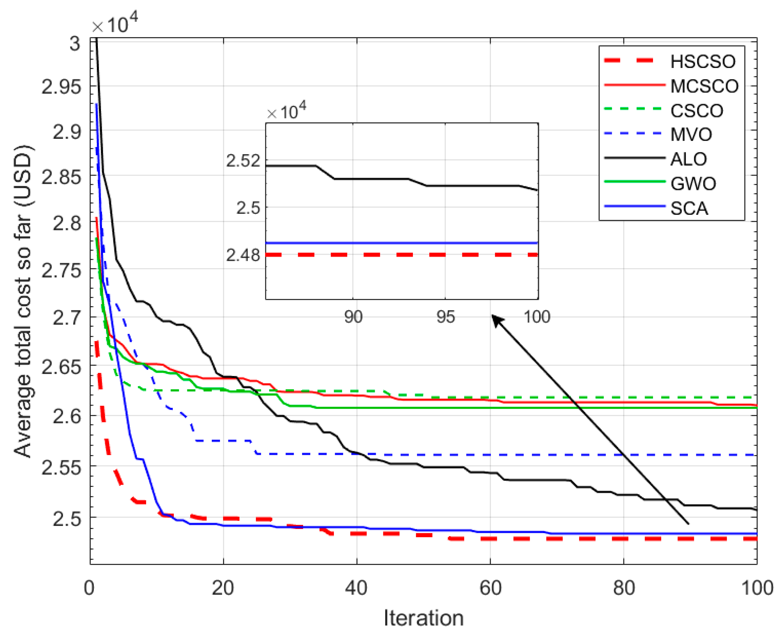
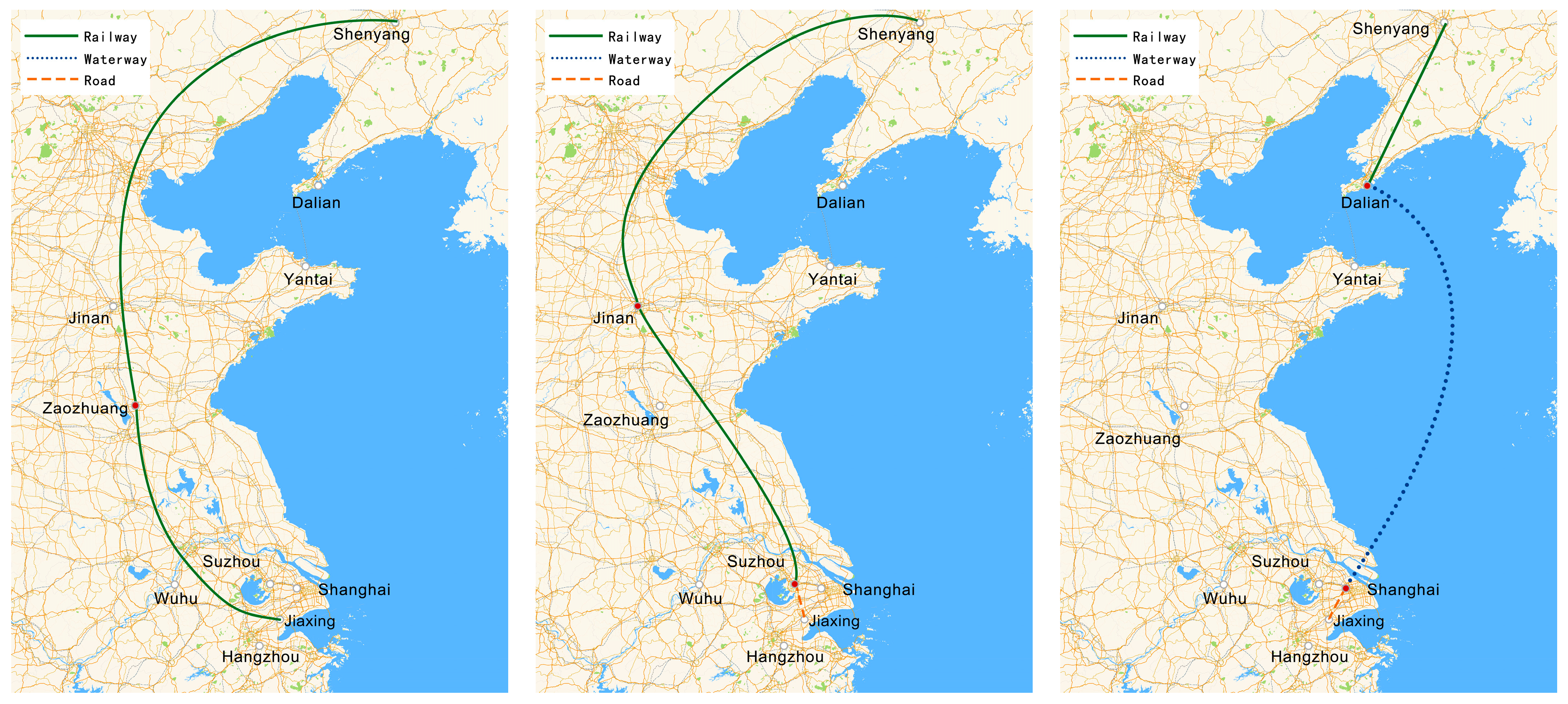
6.2. Analysis of Experimental Results

W substituted the relevant parameters into the model constructed in Chapter 2. Then, we used the MVO [30], ALO [31], SCA [32], GWO [33], SCSO [17], MSCSO [20], and HSCSO algorithms to solve the model separately. The parameter settings of all of the algorithms are the same as those in Table 2, which refers to the CEC2015 benchmark suite. In the modeling of the SCSO algorithm, the problem dimension is explicitly defined as twice the number of cities, representing different city nodes and transportation modes. Each algorithm was repeated 500 times, and the iterative results in this example are illustrated in Figure 6, where the vertical axis represents the average value of the total cost. The optimal delivery routes and lowest costs obtained are shown in Figure 6 and

Table 6. Detailed experimental results.

Algorithm	Path	Modes	Min Cost (USD)	Mean Cost (USD)	Std Cost (USD)
HSCSO	Shenyang–Dalian –Shanghai–Jiaxing	Railway–Waterway –Road	24,054.0	24,797.9	650.8
MSCSO	Shenyang–Dalian –Shanghai–Jiaxing	Railway–Waterway –Road	24,054.0	26,097.6	1610.2
SCSO	Shenyang–Jinan –Suzhou–Jiaxing	Railway–Railway –Road	24,441.9	26,179.6	1495.3
MVO	Shenyang–Zaozhuang –Jiaxing	Railway–Railway	24,533.5	25,895.0	1467.2
ALO	Shenyang–Dalian –Shanghai–Jiaxing	Railway–Waterway –Road	24,054.0	25,069.4	731.3
GWO	Shenyang–Jinan –Suzhou–Jiaxing	Railway–Railway –Road	24,441.9	26,562.4	1507.1
SCA	Shenyang–Zaozhuang –Jiaxing	Railway–Railway	24,533.5	24,846.6	908.2

.

As the test results show, all the algorithms (HSCSO, MSCSO, SCSO, MVO, ALO, GWO, and SCA) obtained the feasible transportation path. Among them, HSCSO, MSCSO, and ALO all found the optimal transportation path with a minimum total cost of 24,054.0 USD. However, the average solution value of HSCSO in each experiment was superior to that of the other algorithms, indicating that HSCSO has a stronger global search capability and consistently finds solutions close to the optimum in different experiments. Moreover, the significantly lower standard deviation of HSCSO suggests that it has good robustness. From the convergence condition, we can see that the initial solution cost of HSCSO is already minimized, benefiting from the optimization of the initial population through Logistic–Tent chaotic mapping. And among the seven algorithms, HSCSO takes more iterations to reach convergence than SCSO, MVO, and GWO. This is mainly because the lens opposition-based learning strategy is introduced in the proposed algorithm during the iteration process, which increases the richness of the population. In addition, the introduction of bellicosity factors and elite cross-pools also accelerates the convergence of the algorithm to a certain extent, alleviating the problem of being difficult to converge. For offline path planning problems, in order to obtain a better result, a longer algorithm running time is acceptable. In general, HSCSO balances the requirements of the convergence accuracy and convergence speed, and has effectiveness and superiority in reducing costs through multimodal transport route planning. The detailed comparison of the costs of each algorithm solution is shown in Figure 7. The optimal path diagrams solved by MVO, SCSO, and HSCSO are shown in Figure 8.

From the comparison, it can be observed that the result of HSCSO makes full use of different modes of transportation and increases the transit cost, but greatly reduces the transportation cost. Equally important, the route planning results of HSCSO effectively suppressed fuel consumption and carbon emissions. While multiple cases of mode-switching in transportation inevitably generates carbon emissions, HSCSO achieved a balance between cost reduction and emission reduction, which is highly consistent with the needs of green logistics. However, its time penalty cost is not the lowest because changing the mode of transportation, which can increase transportation flexibility, can also generate a transit time and waiting time caused by water and railway timetables, but its time penalty is acceptable relative to the reduction in transportation costs. Therefore, it is necessary to introduce a time penalty cost containing a hybrid embedded time window in vehicle multimodal transport.

7. Conclusions

In order to solve the difficulty of balancing different costs and transport times of multimodal transportation and adapt to the needs of green logistics, this paper proposes a green vehicle comprehensive multimodal transportation model, which considers transportation, transit, quality damage, fuel consumption, carbon emission, and time penalty costs with the introduction of the road congestion index and a hybrid embedded time window, and can well-describe the scenario of green multimodal transport. Then, a new improved sand cat optimization algorithm HSCSO is proposed to solve the model. The following conclusions can be drawn about the algorithm: First, to address the drawbacks of the completely randomly generated initial sand cat population, the Logistic–Tent chaotic map is used to optimize the initial positions of the sand cats, thereby broadening the initial search space. Second, to further enhance the convergence ability of the algorithm, so as to balance the convergence speed and convergence accuracy of the algorithm, the momentum–bellicose strategy and elite crossover pool are introduced to enhance the algorithm’s early search ability and mid-to-late convergence ability. Third, for the problem that the SCSO algorithm falls into local extreme values, the adaptive lens opposition-based learning strategy is introduced, so that the algorithm can jump out of the local extreme value multiple times. Next, 10 benchmark functions were tested in 30 dimensions and 100 dimensions, respectively, proving that the HSCSO algorithm has a good optimization effect and convergence accuracy. Finally, the effectiveness of the proposed model and algorithm in planning the path with the lowest cost is verified by practical multimodal vehicle transportation. In addition, because of its efficient search performance, the algorithm can be applied to system optimization in some engineering fields, such as aircraft trajectory optimization, urban traffic signal control, and power system scheduling.

References

1. Beškovnik, B.; Twrdy, E. Green logistics strategy for South East Europe: To improve intermodality and establish green transport corridors. Transport 2012, 27, 25–33. [Google Scholar] [CrossRef]
2. Karam, A.; Jensen, A.J.K.; Hussein, M. Analysis of the barriers to multimodal freight transport and their mitigation strategies. Eur. Transp. Res. Rev. 2023, 15, 43. [Google Scholar] [CrossRef]
3. Laurent, A.B.; Vallerand, S.; van der Meer, Y.; D’Amours, S. CarbonRoadMap: A multicriteria decision tool for multimodal transportation. Int. J. Sustain. Transp. 2020, 14, 205–214. [Google Scholar] [CrossRef]
4. Liu, S. Multimodal transportation route optimization of cold chain container in time-varying network considering carbon emissions. Sustainability 2023, 15, 4435. [Google Scholar] [CrossRef]
5. Bazaluk, O.; Kotenko, S.; Nitsenko, V. Entropy as an objective function of optimization multimodal transportations. Entropy 2021, 23, 946. [Google Scholar] [CrossRef]
6. Hu, Z.A.; Cai, J.; Luo, H. Optimization of multimodal transportation routes under mixed uncertainties. J. Beijing Jiaotong Univ. 2023, 47, 32–40. [Google Scholar]
7. Dorigo, M.; Caro, G.D. Ant colony optimization: A new meta-heuristic. In Proceedings of the 1999 Congress on Evolutionary Computation (CEC99), Washington, DC, USA, 6–9 July 1999; pp. 1470–1477. [Google Scholar]
8. Kennedy, J.; Eberhart, R. Particle swarm optimization. In Proceedings of the ICNN’95-International Conference on Neural Networks, Perth, WA, Australia, 27 November–1 December 1995; pp. 1942–1948. [Google Scholar]
9. Bertsimas, D.; Tsitsiklis, J. Simulated annealing. Stat. Sci. 1993, 8, 10–15. [Google Scholar]
10. Holland, J.H. Genetic algorithms. Sci. Am. 1992, 267, 66–73. [Google Scholar] [CrossRef]
11. Gendreau, M.; Potvin, J.Y. Tabu search. In Search Methodologies: Introductory Tutorials in Optimization and Decision Support Techniques; Springer: Berlin/Heidelberg, Germany, 2005; pp. 165–186. [Google Scholar]
12. Piao, C.; Hu, H.; Zhang, Y. Logistics distribution vehicle path planning research. In Proceedings of the 2020 IEEE International Conference on Artificial Intelligence and Information Systems (ICAIIS), Dalian, China, 20–22 March 2020; pp. 396–399. [Google Scholar]
13. Leng, K.; Li, S. Distribution path optimization for intelligent logistics vehicles of urban rail transportation using VRP optimization model. IEEE Trans. Intell. Transp. Syst. 2021, 23, 1661–1669. [Google Scholar] [CrossRef]
14. SteadieSeifi, M.; Dellaert, N.; Van Woensel, T. Multi-modal transport of perishable products with demand uncertainty and empty repositioning: A scenario-based rolling horizon framework. EURO J. Transp. Logist. 2021, 10, 100044. [Google Scholar] [CrossRef]
15. Kiani, F.; Seyyedabbasi, A.; Aliyev, R.; Shah, M.A.; Gulle, M.U. 3D path planning method for multi-UAVs inspired by grey wolf algorithms. J. Internet Technol. 2021, 22, 743–755. [Google Scholar] [CrossRef]
16. Seyyedabbasi, A.; Kiani, F. Sand Cat swarm optimization: A nature-inspired algorithm to solve global optimization problems. Eng. Comput. 2023, 39, 2627–2651. [Google Scholar] [CrossRef]
17. Adegboye, O.R.; Feda, A.K.; Ojekemi, O.R.; Agyekum, E.B.; Khan, B.; Kamel, S. DGS-SCSO: Enhancing Sand Cat Swarm Optimization with Dynamic Pinhole Imaging and Golden Sine Algorithm for improved numerical optimization performance. Sci. Rep. 2024, 14, 1491. [Google Scholar] [CrossRef]
18. Kiani, F.; Nematzadeh, S.; Anka, F.A.; Findikli, M.A. Chaotic sand cat swarm optimization. Mathematics 2023, 11, 2340. [Google Scholar] [CrossRef]
19. Lou, T.; Yue, Z.; Chen, Z.; Qi, R.; Li, G. A hybrid multi-strategy SCSO algorithm for robot path planning. Res. Sq. 2024; preprint. [Google Scholar] [CrossRef]
20. Wu, D.; Rao, H.; Wen, C.; Jia, H.; Liu, Q.; Abualigah, L. Modified sand cat swarm optimization algorithm for solving constrained engineering optimization problems. Mathematics 2022, 10, 4350. [Google Scholar] [CrossRef]
21. Erdelić, T.; Carić, T.; Erdelić, M.; Tišljarić, L.; Turković, A.; Jelušić, N. Estimating congestion zones and travel time indexes based on the floating car data. Comput. Environ. Urban Syst. 2021, 87, 101604. [Google Scholar] [CrossRef]
22. He, F.; Yan, X.; Liu, Y.; Ma, L. A traffic congestion assessment method for urban road networks based on speed performance index. Procedia Eng. 2016, 137, 425–433. [Google Scholar] [CrossRef]
23. Liu, X.; Chen, Y.L.; Por, L.Y.; Ku, C.S. A systematic literature review of vehicle routing problems with time windows. Sustainability 2023, 15, 12004. [Google Scholar] [CrossRef]
24. Budiyanto, M.A.; Fernanda, H. Risk assessment of work accident in container terminals using the fault tree analysis method. J. Mar. Sci. Eng. 2020, 8, 466. [Google Scholar] [CrossRef]
25. Yin, N. Multiobjective optimization for vehicle routing optimization problem in low-carbon intelligent transportation. IEEE Trans. Intell. Transp. Syst. 2022, 24, 13161–13170. [Google Scholar] [CrossRef]
26. Demir, E.; Hrušovský, M.; Jammernegg, W.; Van Woensel, T. Green intermodal freight transportation: Bi-objective modelling and analysis. Int. J. Prod. Res. 2019, 57, 6162–6180. [Google Scholar] [CrossRef]
27. Zhu, C.; Li, S.; Lu, Q. Pseudo-random number sequence generator based on chaotic logistic-tent system. In Proceedings of the 2019 IEEE 2nd International Conference on Automation, Electronics and Electrical Engineering (AUTEEE), Shenyang, China, 22–24 November 2019; pp. 547–551. [Google Scholar]
28. Zhang, H.; Liu, F.; Zhou, Y.; Zhang, Z. A hybrid method integrating an elite genetic algorithm with tabu search for the quadratic assignment problem. Inf. Sci. 2020, 539, 347–374. [Google Scholar] [CrossRef]
29. Yu, F.; Guan, J.; Wu, H.; Chen, Y.; Xia, X. Lens imaging opposition-based learning for differential evolution with cauchy perturbation. Appl. Soft Comput. 2024, 152, 111211. [Google Scholar] [CrossRef]
30. Mirjalili, S.; Jangir, P.; Mirjalili, S.Z.; Saremi, S.; Trivedi, I.N. Optimization of problems with multiple objectives using the multi-verse optimization algorithm. Knowl. Based Syst. 2017, 134, 50–71. [Google Scholar] [CrossRef]
31. Mirjalili, S. The ant lion optimizer. Adv. Eng. Softw. 2015, 83, 80–98. [Google Scholar] [CrossRef]
32. Rizk-Allah, R.M.; Hassanien, A.E. A comprehensive survey on the sine–cosine optimization algorithm. Artif. Intell. Rev. 2023, 56, 4801–4858. [Google Scholar] [CrossRef]
33. Mirjalili, S.; Mirjalili, S.M.; Lewis, A. Grey wolf optimizer. Adv. Eng. Softw. 2014, 69, 46–61. [Google Scholar] [CrossRef]
Figure 1. The congestion index for the entire road ( C g i = 1.6, C g j = 2.0, S i j k = 200, ω = 0.03).
Applsci 14 08024 g001
Figure 2. Schematic diagram of the hybrid embedded time window.
Applsci 14 08024 g002
Figure 3. The position of the sand cat group in t-th iteration.
Applsci 14 08024 g003
Figure 4. Comparison between the initial and optimized population.
Applsci 14 08024 g004
Figure 5. Convergence curves for ten benchmark functions.
Applsci 14 08024 g005aApplsci 14 08024 g005b
Figure 6. The best results of HSCSO, MSCSO, CSCO, MVO, ALO, GWO, and SCA.
Applsci 14 08024 g006
Figure 7. Comparison of costs for each solution.
Applsci 14 08024 g007
Figure 8. Path planning result of MVO, SCSO, and HSCSO.
Applsci 14 08024 g008