Forecasting Cost Risks of Corn and Soybean Crops through Monte Carlo Simulation

Featured Application

Monte Carlo Simulations can be used to forecast cost risks in agribusinesses, supporting better decision-making. Such risks should be minimized to optimize production costs, namely, materials, labor, and overhead costs, which can vary significantly and differently due to different cost behaviors. Forecasting costs using Monte Carlo simulations can provide a clear view of the expected cost range for the subsequent periods, enabling farmers to make better strategic planning and resource allocation decisions.

Abstract

Considering that investing in the production of corn and soybeans is conditioned by production costs and several risks, the objective of this research work was to develop a simulation model for the prediction of the production costs of these commodities, considering the variability and correlation of key variables. The descriptive analysis of the data focused on measures such as mean, standard deviation, and coefficient of variation. To evaluate the relationship between commodity and input prices, Spearman’s demonstration coefficient and the coefficient of determination (R²) were used. A Monte Carlo simulation (MCS) was used to evaluate the variation in production costs and net revenues. The Predictor tool was used to make predictions based on historical data and time series models. This study was made for the period between 2018 and 2022 based on data provided by fifty companies from the state of São Paulo, Brazil. The results showed that the production cost/ha of corn faces a high-cost risk, particularly when production and market conditions are characterized by high levels of volatility, uncertainty, complexity, and ambiguity. The model proposed forecasts prices more accurately, as it considers the variation in the costs of inputs that most significantly influence the costs of corn and soybean crops.

1. Introduction

Worldwide, corn and soybeans stand out among the main commodities of agribusiness. For example, in Brazil, over the last decade, they have been the most produced and exported agricultural commodities, contributing to the Brazilian trade surplus with export revenues exceeding USD 53.889 billion in 2021 [1]. The competitiveness of these crops in international markets is correlated to long-term production and transportation costs, as well as export policies and fluctuations in exchange rates, among other aspects [2,3]. In early 2022, for instance, the prices of corn and soybean crops increased due to higher global demand [3], rising fertilizer costs [4,5], and the drought in South America caused by the La Niña phenomenon. The war in Ukraine also contributed to the increase in production costs for all commodities [5].

Although Meade et al. [2] have extensively researched production costs and competitiveness of soybean and corn exports in the main producing countries, such as Argentina, Brazil, and the United States, there is a lack of application of predictive models that integrate the variability of inputs and production costs and the market volatility. The use of a Monte Carlo Simulation may offer a more robust and dynamic analysis of fluctuations in production costs, thus addressing a gap present in current research.

According to several predictions, the high prices of soybeans and corn were expected to continue to become higher during several periods [6]. Given such a scenario of increased costs, forecasts of production costs are particularly important for decision-makers in agribusiness [7,8,9]. According to Pitrova et al. [10] and Amorim et al. [11], computational simulation has proven to be an appropriate support tool for decision-making in this context. Meade et al. [2] highlighted the costs related to logistics, land, and storage, while Oliveira et al. [5] considered also the costs of fertilizers, seeds, fuel, and pesticides, among others.

Oliveira et al. [5] recognized the importance of inputs such as fertilizers and seeds in computing an accurate production cost of agricultural products. However, they have not comprehensively explored the complex interactions between these factors and their impact on cost predictability under different economic scenarios. There, is, indeed, a gap in terms of studies that offer an integrated approach that, in addition to identifying these interactions, can quantify them using probabilistic simulation models.

Furthermore, the analysis of the relationship among these variables is fundamental to understanding and improving the performance of agribusinesses, namely, providing predictions for short-, medium-, and long-term decision-making [5,11]. The literature offers a significant number of studies in different countries focused on the production costs of corn and soybeans [2,12,13,14], as well as others about economic feasibility and risk analysis through case studies [15,16] and some on the analysis of soybean and corn prices [17,18]. Krah [17] studied corn price variability and its implications for changes in land use and forest loss in Ghana, highlighting economic factors crucial to agricultural sustainability. However, there is still a lack of research that connects these price variabilities to predictive cost models in the main producers, such as Brazil.

Several researchers have explored the competitiveness of the main soybean and corn producers in the international market, highlighting factors such as government policies, production costs, economic challenges, production systems, and the importance of improving agricultural infrastructure. Although they provide relevant information about current conditions and comparisons between countries, little work exists on guidelines that can directly assist producers in making strategic decisions, which limits the practical application of research for agricultural planning. Thus, there is a gap and a need for models focused on the expected costs and their trends for the near future. Therefore, it is important to identify the inputs that significantly influence the price and cost variations of corn and soybean crops.

This study focused on data obtained from companies in the state of São Paulo due to the significant presence of both crops in this region. The variation and correlation among inputs, prices, and production costs of corn and soybeans were analyzed, as well as how these factors impact predictions for the next harvests.

Simulation and mathematical models have been used to optimize soybean production and business processes, price predictability, and other factors. Indeed, simulation applications in agribusiness have shown that models based on intelligent systems can be highly suitable for a wide range of applications in various fields [19,20]. Unlike equations structured in linear, quadratic, or other predetermined formats, these models offer significantly greater adaptability to response data. They surpass the limitations of traditional statistical models, for instance. Using a Monte Carlo Simulation (MCS), several possible scenarios of production costs can be considered, including uncertainty and variability in the prices of selected key variables. By integrating the cost trend analysis with an MCS, it can be possible to understand and predict how fluctuations in input and labor markets influence the final production cost of corn and soybeans.

Rather than providing static estimates, a Monte Carlo Simulation accounts for the uncertainties surrounding each variable, conducting multiple simulations to derive a probabilistic distribution of potential outcomes, thereby taking into consideration market volatility and uncertainties [5,21,22]. It is worth noting that this methodology is still relatively underexplored in the context of agricultural products. However, it is of crucial importance because it enhances the accuracy of estimates.

The model proposed in this paper supports decision-making by enabling better economic and financial planning and strategic decision-making. For instance, it helps select the best crops to plant and facilitates negotiations and contracts involving the purchase of inputs and labor. Furthermore, it reduces the risk of financial losses and allows for the adoption of strategies that may contribute to a higher competitiveness in the production and export of these crops.

The production of corn and soybeans has been growing significantly in recent years asking for a better understanding of its price dynamics. In an industry highly dependent on fluctuations in input prices and market volatility, the ability to accurately predict costs is essential to ensure economic sustainability. Indeed, forecasting cost risks and their causes support better decision-making in agribusinesses.

2. Materials and Methods

Monte Carlo (MC) simulations were made to evaluate the variability and correlation of production costs considering data provided by fifty companies in the state of São Paulo, Brazil. An MC simulation is particularly suitable for this type of analysis, as it models the uncertainty and variability of the main variables involved, generating different cost scenarios, and enabling a better understanding of the risks, rather than relying on single estimates, or simple averages. Furthermore, Spearman correlation coefficients and ARIMA models were used to validate and refine the predictions, ensuring greater precision in the results obtained. The analysis considered data between 2018 and 2022, allowing a detailed analysis of cost risks over time.

2.1. Case Study

The cultivation of corn in São Paulo plays an important role in the state’s economy. In 2022, the estimated corn production in São Paulo was 4.8 million tons [23]. The contribution of corn cultivation to the state’s agriculture increased from 3.9% in 2017 to 6.1% in 2021 [24] and Brazilian exports experienced significant growth, leading to important changes in the domestic market. In 2022, the state of São Paulo contributed to the international shipment of 978,268.18 tons, which represents 2.3% of Brazilian corn exports [25]. São Paulo combines good conditions for crop production, modern logistics facilities, and access to internal and external markets, contributing to shorter, thus, more competitive and sustainable supply chains, and the valorization of local production for conditions of modern agribusinesses [26].

The cultivation of soybeans in the state of São Paulo is relatively more recent but has experienced significant growth since the 1990s. The planted area of soybeans in the state increased from approximately 580,000 hectares in the 2001/2002 crop season to 1263.6 thousand hectares in the 2021/2022 period [27]. Soybeans now represent the second largest crop in the state’s agriculture, accounting for 12.1% of the total cultivated area, second only to sugarcane, which remains the primary crop with a share of 48.3% [28]. In 2022, São Paulo exported 5,059,820.089 tons of soybeans, which represents 6.4% of the total export of this commodity [25]. The main destinations for these exports were China, Iran, Thailand, and Spain [27].

2.2. Data Collection

The data were obtained from a database provided by the Institute of Agricultural Economics-IEA [29], using the questionnaire on Average Prices Paid by Agriculture in the state of São Paulo. This questionnaire collects the selling prices of inputs used by farmers, using data from retailers located in the state of São Paulo, on a monthly basis.

IEA adopts a random sample that includes retailers, cooperatives, and manufacturers, who are invited to provide information on selling prices. Data collection is carried out through questionnaires sent by email, on-site visits, and telephone interviews. Additionally, some research is performed on the websites of governmental agencies, such as the National Agency of Petroleum, Natural Gas, and Biofuels, and the National Association of Transportation and Logistics. For the present study, the sample includes data obtained from 50 companies in the state of São Paulo, and the data collection was developed from January 2018 to December 2022 (n = 60).

The data include the prices in USD for diesel fuel, Trifloxystrobin Tebuconazole fungicide, Glyphosate herbicide, Thiamethoxam Lambda-Cyhalothrin insecticide, Dolomitic limestone corrective, NPK 05-25-25 fertilizer, Potassium chloride fertilizer, USD exchange rate, Soybean price per bag, Corn price per bag, Soybean seed, Corn seed, Tractor operator labor, Daily labor, and Urea fertilizer. Given the wide variety of fertilizers available in the market, we only included the main fertilizers used in the cultivation of corn and soybeans.

2.3. Descriptive Analysis

The descriptive analysis was focused on the minimum and maximum values, arithmetic mean, total range, variance, standard deviation, coefficient of variation (low < 10%, medium between 10 and 20%, high between 20 and 30%, and very high > 30%), skewness (symmetric variation = 0; >0 positive <0 negative), and kurtosis (leptokurtic: K < 0.263; mesokurtic: K = 0.263; and platykurtic: K > 0.263).

2.4. Spearman Correlation Coefficient (r) and Coefficient of Determination (R²)

The Spearman correlation coefficient (r) was used to measure the existence and degree of correlation between the price (in USD) of corn or soybean per bag (independent variable) and the price (in USD) of the other dependent variables used in this study, collected monthly. Spearman’s rank correlation (ρ) is an interdependence technique used when no variable or group of variables is treated as dependent or independent [30]. Spearman employs a correlation estimate based on ranking, meaning that variables are categorized in consecutive order according to the observed values.

The result of this analysis is presented as a dimensionless index, with values ranging from −1.0 to 1.0, reflecting the strength of a linear relationship between two sets of data. If the value of r is equal to 1, there is a perfect positive correlation between the two. If the value of r is equal to −1, there is a perfect negative correlation [28,31].

The coefficient of determination (R²) is the square of the Spearman correlation coefficient and is a measure of the quality of the model fit. It describes the proportion of variability in one variable that is explained by the variability in the other variable. The value of R² can range from 0 to 1, and, since it is difficult to find a perfect correlation in practice, higher values are associated with lower error variance. In this study, R² values ≥ 0.7 were considered to indicate a strong correlation in the interpretation of the correlation data [28].

2.5. Monte Carlo Simulation

The main production costs per bag of soybean and corn were investigated in relation to all the variables through cumulative frequency analysis using the Crystall Ball software version 11.1.2.1.0 [32]. To analyze the probability of cost variation and gross net revenue, a Monte Carlo simulation (MCS) was used through a stochastic approach [5,15,21,33]. The average result of the MCS for each variable was obtained using Equation (1).

$${\mathrm{a}}_{\mathrm{m}}={\displaystyle \frac{1}{\mathrm{n}}}\sum _{\mathrm{i}=1}^{\mathrm{n}}{\mathrm{x}}_{\mathrm{i}}$$

(1)

where a_m is the average result of the MCS for the variable, x represents the individual result of each simulated iteration, and n is the number of simulations (iterations).

a_m is the normalization factor, indicating that the sum of the results is divided by the number of simulations carried out.

1/r is the estimated value or the average of the simulated results. It can represent an estimate of the expected value of a variable or the average result of several simulations.

N is the total number of simulations, the average can be given dividing by N.

x_i: represents the values obtained in different simulations or samples.

Dividing by the total number of simulations (or the normalization factor, if r) gives the average of the simulated results, which is an estimate of the expected value of the model or system. The formula is used to estimate the mean or expected value of a random variable that is the result of the simulation.

In this research, 50,000 iterations were made, which is the maximum number of iterations provided by the software and it is a significant number for this specific problem. Similar approaches were used in several studies, e.g., [5,21]. To forecast future events, the Predictor tool version 11.1.2.1.0 was used, which is a stochastic simulation tool available from the software. It was used to make predictions based on time series data by analyzing historical data from which it was possible to identify trends and seasonal patterns. These insights were then used to forecast the most probable outcomes.

The scenarios were forecasted using the software for a period of 24 months, based on data from 2018 to 2022. The MCS uses quantitative methods based on time series for forecasting [32], namely, Simple Exponential Smoothing (SES), Autoregressive Integrated Moving Average (ARIMA), Damped Trend Non-Seasonal (DTN-S), Double Moving Average (DMA), Non-Seasonal Smoothed Trend (TANS), and Double Exponential Smoothing (DES). The distribution used by the predictor was the triangular distribution. This model was employed due to the low dispersion of the values presented in the descriptive analysis of the MCS.

Each method has its strengths and is chosen based on the characteristics of the time series data (e.g., trend, seasonality, stationarity).

2.5.1. Simple Exponential Smoothing (SES)

SES is used for time series forecasting when the data show no trend or seasonal patterns. It smooths the data using a weighted average of past observations. More recent observations are given more weight—Equation (2).

$${\widehat{\mathrm{y}}}_{\mathrm{t}+1}={\mathsf{\alpha }\mathrm{y}}_{\mathrm{t}}+\left(1-\mathsf{\alpha }\right)\widehat{\mathrm{y}}$$

(2)

where Equation (2) is the forecast for the next period, y_t is the actual value at time t, and α (with 0 < α < 1) is the smoothing parameter.

2.5.2. Autoregressive Integrated Moving Average (ARIMA)

ARIMA is used for forecasting time series data that may have a trend but no seasonal component. It combines autoregressive (AR) terms, differencing (I) to make the series stationary, and moving average (MA) terms to model the time series—Equation (3).

$$\mathrm{\varphi }\left(\mathrm{B}\right){\left(1-\mathrm{B}\right)}^{\mathrm{d}}{\mathrm{y}}_{\mathrm{t}}=\mathsf{\theta }\left(\mathrm{B}\right){\in }^{\mathrm{t}}$$

(3)

where Φ(B) are polynomial operators for the AR and MA components, respectively, d is the differencing order, and ϵ^t is the white noise error term.

2.5.3. Damped Trend Non-Seasonal (DTN-S)

DTN-S is used for time series data with a trend but no seasonal pattern, where the trend is expected to diminish over time. It extends the Holt’s linear trend model by introducing a damping parameter to reduce the influence of the trend over time—Equation (4).

$${\widehat{\mathrm{y}}}_{\mathrm{t}+\mathbf{k}}={\mathrm{l}}_{\mathrm{t}}+\mathrm{\varphi }\mathrm{t}·{\mathrm{b}}_{\mathrm{t}}$$

(4)

where l_t is the level, b_t is the trend, ϕ is the damping parameter, and t is the time period.

2.5.4. Double Moving Average (DMA)

DMA is used to smooth out time series data by averaging data points over a specified period, and then applying another moving average to the result. It involves applying a simple moving average twice, first to the raw data and then to the smoothed data—Equations (5) and (6).

$${\mathrm{S}\mathrm{M}\mathrm{A}}_1\left(\mathrm{t}\right)={\displaystyle \frac{1}{\mathrm{m}}}\sum _{\mathrm{i}=\mathrm{t}-\mathrm{m}+1}^{\mathrm{t}}{\mathrm{y}}_{\mathrm{i}}$$

(5)

$${\mathrm{S}\mathrm{M}\mathrm{A}}_2\left(\mathrm{t}\right)={\displaystyle \frac{1}{\mathrm{m}}}\sum _{\mathrm{i}=\mathrm{t}-\mathrm{m}+1}^{\mathrm{t}}{\mathrm{S}\mathrm{M}\mathrm{A}}_1(\mathrm{i})$$

(6)

where ${\mathrm{S}\mathrm{M}\mathrm{A}}_1$(t) is the first moving average, ${\mathrm{S}\mathrm{M}\mathrm{A}}_2$(t) is the second moving average, and m is the period length.

2.5.5. Non-Seasonal Smoothed Trend (TANS)

TANS is used for time series data with a smoothed trend but no seasonal component. It involves smoothing the time series to account for trends while ignoring seasonality. This can vary, but typically involves smoothing techniques that adjust for trend while ignoring seasonal fluctuations, such as a moving average or smoothing spline.

2.5.6. Double Exponential Smoothing (DES)

DES is used for time series data with a trend but no seasonality. It extends SES by adding a component to model the trend in the data. It provides forecasts by combining the level and trend components—Equations (7)–(9).

$${\widehat{\mathrm{y}}}_{\mathrm{t}+1}={\mathrm{l}}_{\mathrm{t}}+{\mathrm{b}}_{\mathrm{t}}$$

(7)

$${\mathrm{l}}_{\mathrm{t}}={\mathsf{\alpha }\mathrm{y}}_{\mathrm{t}}+\left(1-\mathsf{\alpha }\right)({\mathrm{l}}_{\mathrm{t}-1}+{\mathrm{b}}_{\mathrm{t}-1})$$

(8)

$${\mathrm{b}}_{\mathrm{t}}=\mathrm{B}\left({\mathrm{l}}_{\mathrm{t}}-{\mathrm{l}}_{\mathrm{t}-1}\right)+\left(1-\mathsf{\beta }\right){\mathrm{b}}_{\mathrm{t}-1}$$

(9)

where α is the smoothing parameter for the level, β is the smoothing parameter for the trend, l_t is the level at time t, and b_t is the trend at time t.

3. Analysis and Discussion of Results

3.1. Descriptive Analysis

The results of the descriptive analysis (

Table 1. Descriptive measures referring to variables related to the cost of production of corn and soybeans (USD) from January 2018 to December 2022.

	DOIL	FUTT	HEGL	INTL	DLLC	NPKF	DLR	SOY	COR	SOYS	CORS	TRAC	DAI	PCF	URF
n	60	60	60	60	60	60	60	60	60	60	60	60	60	60	60
MIN	0.57	16.95	18.91	29.59	14.8	278.4	3.18	12.61	5.66	0.57	2.33	302.26	13.25	352.38	339.04
MAX	1.41	22.66	92.02	48.68	40.98	1205.24	5.67	36.51	18.53	2.29	4.31	387.01	18.9	1256.63	1201.48
RANGE	0.84	5.71	73.11	19.09	26.18	926.84	2.49	23.9	12.87	1.72	1.98	84.75	5.65	904.25	862.43
MEAN	0.80	19.28	36.22	38.17	25.28	576.043	4.66	22.57	11.27	1.332	3.299	2.83	15.37	602.53	580.38
VAR	0.0586	3.1021	625.35	24.85	64.30	104,435	0.5986	72.132	20.392	0.3075	0.114	706.85	2.81	113,307.91	85,958.13
SD	0.24	1.7613	25.0071	4.9851	8.0191	323.1645	0.77	8.4931	4.5157	0.55	0.33	26.58	1.67	336.61	293.18
CV	30.1%	9.1%	69.0%	13.1%	31.7%	56.1%	16.6%	37.6%	40.0%	41.6%	10.2%	7.8%	10.9%	55.8%	50.5%
SKEW (g1)	1.2158	0.5324	1.3291	0.3488	0.73	0.947	−0.265	0.2153	0.2287	0.4712	−0.2119	0.2294	0.6285	1.0545	1.0692
KURT (g2)	0.0765	−1.2306	0.026	−0.7111	−0.7596	−0.8431	−1.443	−1.7728	−1.693	−1.4971	1.1549	−1.2933	−0.8398	−0.7136	−0.5489

n: sample size (monthly data collected from 2018 to 2022); MIN: minimum; MAX: maximum; RANGE: total range; MEAN: arithmetic mean; VAR: variance; SD: standard deviation; CV: coefficient of variation; SKEW: skewness; KURT: kurtosis; DOIL: diesel oil (L); FUTT: fungicide trifloxystrobin tebuconazole (L); HEGL: herbicide glyphosate (L); INTL: insecticide thiamethoxam lambda-cyhalothrin (L); DLLC: dolomitic limestone corrective (ton); NPKF: NPK 05-25-25 fertilizer (ton); DLR: dollar exchange rate; SOY: soybean bag (kg); COR: corn bag (kg); SOYS: soybean seed (kg); CORS: corn seed (kg); TRAC: tractor driver hours (h); DAI: daily worker hours (h); PCF: potassium chloride fertilizer (kg); URF: urea fertilizer (kg).

) revealed a significant variability in the total range of all the variables chosen for this study.

This fact can be explained by the increase in prices of inputs used in the production of corn and soybeans from 2018 to 2022. The 59% appreciation of the dollar is related to the rise in prices of fertilizers, soil amendments, and agricultural pesticides during the studied period [34,35,36,37,38], as the dollar is the currency used in international transactions, including the trade of agricultural inputs imported by farmers.

In addition to these factors, uncertainties caused by the COVID-19 pandemic have led to imbalances between supply and demand of inputs in the global market, which have influenced significant fluctuations in prices of fertilizers, herbicides, fuel, and other inputs analyzed in this study [39]. The uncertainties stemming from the pandemic have affected all sectors of agribusiness, from production to distribution and marketing, resulting in negative economic impacts across all segments, particularly in input costs [4,40].

In contrast, the increase in the value of the dollar also stimulated the exports of corn and soybeans, thereby pushing the domestic supply and further raising prices. Given such a scenario, it is crucial for the agricultural sector to be aware and anticipate exchange rate fluctuations and seek alternatives to mitigate the impact of changes in the dollar exchange rate on production costs.

The lowest variances and standard deviations were found for the prices of diesel fuel, dollar exchange rate, soybean seed, and corn seed. This indicates that the values of these inputs and the exchange rate did not deviate significantly from the mean during the study period, indicating lower cost risks here.

Indeed, the coefficient of variation results indicated that the prices of the following variables: diesel fuel, glyphosate herbicide, dolomitic limestone corrective, NPK 05-25-25 fertilizer, corn bushel, soybean bushel, soybean seed, potassium chloride fertilizer, and urea fertilizer exhibited a high dispersion. On the other hand, the prices of tiamethoxam lambda-cyhalothrin insecticide, dollar exchange rate, corn seed, and casual labor had a moderate dispersion, while the prices of trifloxystrobin tebuconazole fungicide and tractor operator labor were classified as having low dispersion.

The highest coefficient of variation was found for the glyphosate herbicide. The literature suggests that in addition to the external factors, internal factors such as market demand, production costs, distribution, and sales of each company, as well as government intervention (such as taxation on imported products), influence the costs and consequently the price formation of this herbicide [41].

The lowest coefficient of variation was found in the price of “tractor driver”. Although it showed low dispersion over the study period, costs related to tractor drivers’ such as wages have shown great relevance in the total production costs of corn and soybeans [42,43].

A descriptive analysis of the variables used in this study was made using data collected on their prices (in USD).

No variable exhibited symmetry in the analyzed prices during the period from 2018 to 2022. Positive skewness distributions were found for diesel oil, fungicide trifloxystrobin tebuconazole, herbicide glyphosate, insecticide thiamethoxam lambda-cyhalothrin, dolomitic limestone corrective, fertilizer NPK 05-25-25, soybean bag price, corn bag price, soybean seed, tractor operator labor, daily laborer labor, potassium chloride fertilizer, and urea fertilizer. This means that the prices of these inputs remained above the average for a significant part of the analyzed period, which can be explained by the factors discussed previously. The US dollar and corn seed were the only variables in which prices exhibited negative skewness distributions, meaning that they remained below the average for a significant part of the analyzed period. Despite reaching high values at times, the dollar remained below the average in recent years due to a combination of factors, including a decline in the performance of the US economy, which has not remained as strong due to global instabilities and political tensions [44]. Regarding corn seed, its price in São Paulo is influenced by the price in Sorriso-MT and in Paraguay, as they are, respectively, the main national production areas and the origin of most of the corn imported by Brazil [45].

For the analysis of kurtosis, it was evident that the prices of corn seed exhibited a platykurtic distribution, meaning that the values were more concentrated around the mean. The price of corn seed in São Paulo increased by 120% from 2018 (USD 1827.1) to 2022 (USD 4028.54). This significant variability can be explained by changes in the commodities market and currency fluctuations that affect corn costs [46,47,48].

Regarding the price of the herbicide glyphosate and the price of diesel fuel, the mesokurtic distribution found for these inputs (moderate concentration of values around the mean) may be related to economic and environmental factors related to the production, supply, and demand of these products [41,49]. The remaining variables exhibited a leptokurtic distribution (relatively low concentration of values around the mean). The leptokurtic distribution in the prices of the agricultural inputs studied may have been influenced by the pandemic [39,50], variations in agricultural productivity [51], supply and demand [52], and the price of the dollar [34,37,38].

3.2. Economic Analysis of Corn and Soybeans

The data related to prices, quantity of inputs used in soybean and corn cultivation, production costs, and net profit are presented in

Table 2. Economic analysis of corn and soybeans.

Items	Description	Unit	Crop	Cost/ha (USD)	Cost/ha/Corn (%)	Cost/ha/Soybean (%)
DOIL	36	L/ha	Corn/soybean	29.8	4.7	5.8
FUTT	0.750	L/ha	Corn/soybean	28.9	4.6	5.7
HEGL	5	L/ha	Corn/soybean	36.2	5.8	7.1
INTL	0.750	L/ha	Corn/soybean	28.6	4.6	5.6
DLLC	1	T/ha	Corn/soybean	25.3	4.0	5.0
NPKF	500	T/ha	Corn/soybean	288.0	45.9	56.5
COR	60	kg/ha	Soybean	10.5	NA	NA
SOY	20	kg/ha	Corn	11.3	NA	NA
SOYS	60	kg/ha	Soybean	79.9	NA	15.7
CORS	20	kg/ha	Corn	66.0	10.5	NA
TRAC	2	2 h/ha	Corn/soybean	2.83	0.5	0.6
DAI	2	2 h/ha	Corn/soybean	3.84	0.6	0.8
PCF	100	kg/ha	Corn	60.2	9.6	NA
URF	100	kg/ha	Corn	58.0	9.2	NA
TCOST	NA	ha	Corn	627.7	100	NA
	NA	ha	Soybean	509.5	NA	100
Productivity Data
EPROD	91 bag/ha	60 kg/bag	Corn	11.3	NA	NA
	50 bag/ha	60 kg/bag	Soybean	22.6	NA	NA
Gross Income				USD
Corn		1026.3
Soybean		1128.6

DOIL: diesel; FUTT: fungicide trifloxystrobin tebuconazole; HEGL: herbicide glyphosate; INTL: insecticide thiamethoxam lambda-cyhalothrin; DLLC: dolomitic limestone corrective; NPKF: NPK 05-25-25 fertilizer; dollar exchange rate; SOY: soybean bag; COR: corn bag; SOYS: soybean seed; CORS: corn seed; TRAC: tractor driver hours (h); DAI: daily worker hours (h); PCF: potassium chloride fertilizer; URF: urea fertilizer. TCOST: Total Cost; EPROD: Expected Yield/Productivity; L: liter; T: tonne; ha: hectare; kg: kilogram. h: hours; NA not applicable. Source: São Paulo Banco de Dados [39].

. The ‘description’ column highlights the quantity used for the different inputs, while the ‘crop’ column indicates whether they are used in corn, soybean, or both. The average cost per hectare for the different inputs is also presented. The inputs that contribute more to the total production cost of these crops are NPK 05-25-25 fertilizer (45.9% in corn production and 56.5% in soybean production), soybean seeds (15.7% in soybean production), corn seeds (10.5% in corn production), potassium chloride fertilizer (9.6% in corn production), and urea (9.2% in soybean production).

The average production cost per hectare is USD 627.7 for corn and USD 509.5 for soybean. The Expected Yield/Productivity per hectare for corn and soybean was based on the literature (EPROD in Table 2). In the market, these grains are sold in 60 kg bags, thus, the average production cost per bag is presented. The Gross income was calculated by multiplying the expected productivity by the average price of corn and soybean bags.

The levels of certainty regarding the average production cost per hectare of corn associated with the analyzed variables were calculated using MCS and are presented in the frequency graph presented in Figure 1.

The simulation results presented in Figure 1 show that the average production costs of soybean per hectare in the state of São Paulo ranged between USD 260.00 and USD 420.00, with a level of certainty of 86.4% (blue Figure 1) for an average of USD 340.20 and a standard deviation of USD 53.55, in the period between 2018 and 2022.

These results are based on historical prices. Thus, the analysis conducted can help in the minimization of uncertainty regarding soybean production costs for the state and support decision-making regarding input purchases.

The results obtained in this study are similar to the information published by [53] for the state of São Paulo, specifically the city of Assis, one of the main corn producers’ municipalities in the state. The values provided by Conab are presented in Brazilian Reais and have been converted to US Dollars using the average exchange rate (R$/USD) for each year.

The data used in this analysis were obtained from IPEA data, available from the authors upon request. For comparison purposes, the average calculation was performed considering only the costs of operating expenses, excluding other costs such as storage and charges, among others. The average production cost of soybeans was found to be USD 417.77 during the period between 2019 and 2021.

The levels of certainty of the average production cost per hectare of corn associated with the analyzed variables were calculated using MCS and are presented in the frequency graph (Figure 2).

The simulation results show that the range between USD 600.00 and USD 1150.00 contains the average production costs of corn per hectare in the state of São Paulo, with a level of certainty of 84.7% (blue Figure 2) for an average of USD 870.80 and a standard deviation of USD 192.40, considering the period between 2018 and 2022.

The monitoring data from [54] regarding the production costs of the second corn crop for the years 2019 and 2020 show an average production cost of USD 421.26, represented by the city of Assis. On the other hand, [55] indicates costs in other states in Brazil that corroborate these results, with costs ranging from USD 613.00 to USD 653.00 in the 2018/19 and 2019/20 harvests (using transgenic seeds).

It was observed that the production costs in each municipality and state were influenced by differences in terms of productivity. The costs of high-productivity areas are lower than the costs of low-productivity areas [13]. In addition to productivity, other factors contribute to the observed differences in corn production costs in the different regions, such as climate [56], prices of inputs [57], and technology used [58,59].

The most significant cost elements of corn and soybeans production costs (fertilizers and soil amendments) account for 68.7% and 61.5%, respectively. Equally important are the costs of agricultural inputs (herbicides, insecticides, and fungicides), which amount to 15% and 18.4% for corn and soybeans, respectively.

An alternative to reduce these costs would be the use of Variable Rate Technology (VRT), which means the application of soil amendments and fertilizers according to each point analyzed by the grid or management zone [11]. According to Baio et al. [60], this technique is employed in precision agriculture for the application of inputs and agricultural pesticides, which allows for the optimization of the effectiveness and costs of these inputs. These authors stated that the use of a VRT system proved to be advantageous in agricultural production.

Consumption of inputs and, consequently, the cost of chemical fertilizers, can be reduced using organ mineral fertilizers (combinations of organic sources). Corroborating this, Freitas et al. [61] stated that this type of fertilizer emerges as an alternative for nutrient supply in corn cultivation and contributes to reduced dependence on imported mineral fertilizers, in addition to increased productivity.

Reinforcing this statement, a case study in soybean cultivation in Brazil demonstrated that organ mineral fertilizers proved to be effective, achieving productivity of 3648.96 kg/ha, and could be an alternative to traditional mineral fertilization [62]. There is evidence from different countries on the effectiveness of using organ mineral fertilizers in agricultural production, e.g., [63,64].

Another possibility to reduce the total cost regarding the use of agricultural pesticides, which has shown significant growth, is the use of biological alternatives. It has been reported that the use of biological control is growing at a rate of more than 15% per year, since 2005 [65]. There is an increase in the use of biologic control of 10–15 % a year worldwide, and 30–35 % annually in Brazil, turning Brazil one of the most extensive users of biological control, which includes bioagents, biofertilizers and bio stimulants [66].

To conclude, the gross revenue of corn is 9.1% lower than that of soybeans. This is due to several factors, such as the higher production cost per hectare for corn (18.8%) compared to soybeans, and a 7.6% lower price per 60 kg bag, as mentioned above. However, the average prices (paid to farmers during the studied period) for corn at USD 11.3 and soybeans at USD 22.6 are close to the price levels of September 2020, suggesting stability in prices.

3.3. Spearman Correlation Coefficient (ρ) and Coefficient of Determination (R²)

The Spearman correlation coefficient (ρ) was used to measure the existence and degree of correlation between the price (in USD) of corn or soybean per bag (independent variable) and the price (in USD) of the dependent variables.

The correlation of the prices (in USD) of the selected dependent variables considered in this study (diesel fuel, fungicide Trifloxystrobin Tebuconazole, herbicide Glyphosate, insecticide Thiamethoxam Lambda-Cyhalothrin, Dolomitic Limestone amendment, NPK 05-25-25 fertilizer, exchange rate, soybean seed, corn seed, tractor operator labor, daily laborer labor, Potassium Chloride fertilizer, Urea fertilizer) and the independent variable (corn or soybean price in USD) is presented in

Table 3. Spearman correlation coefficient (p) and coefficient of determination (R²).

DV	IV	p	R2	DC	IV	p	R2	DC
DOIL	Corn	0.72	0.52	Strong	Soy	0.81	0.65	Strong
FUTT	Corn	0.88	0.77 *	Strong	Soy	0.92	0.85 *	very strong
HEGL	Corn	0.65	0.42	moderate	Soy	0.74	0.54	Strong
INTL	Corn	0.79	0.64	Strong	Soy	0.83	0.68	Strong
DLLC	Corn	0.81	0.65	Strong	Soy	0.87	0.77 *	Strong
NPKF	Corn	0.80	0.64	Strong	Soy	0.86	0.75 *	Strong
DLR	Corn	0.79	0.62	Strong	Soy	0.77	0.59	Strong
SOY	Corn	0.92	0.93 *	very strong	Soy	0.97	0.93 *	very strong
SOYS	Corn	0.92	0.93 *	very strong	Soy	0.97	0.93 *	very strong
CORS	Corn	0.15	0.02	negligible	Soy	0.27	0.08	Negligible
TRAC	Corn	0.91	0.83 *	very strong	Soy	0.95	0.90 *	very strong
DAI	Corn	0.87	0.75	Strong	Soy	0.92	0.85 *	very strong
PCF	Corn	0.72	0.54	Strong	Soy	0.81	0.66	Strong
URF	Corn	0.77	0.60	Strong	Soy	0.84	0.70	Strong

DV: dependent variable; IV: Independent variable; p: Spearman Correlation Coefficient; R²: coefficient of determination; DC: degree of correlation; DOIL: diesel; FUTT: fungicide trifloxystrobin tebuconazole; HEGL: herbicide glyphosate; INTL: insecticide thiamethoxam lambda-cyhalothrin; DLLC: dolomitic limestone corrective; NPKF: NPK 05-25-25 fertilizer; DLR: dollar exchange rate; SOY: soybean bag; SOYS: soybean seed; CORS: corn seed; TRAC: tractor driver hours (h); DAI: daily worker hours (h); PCF: potassium chloride fertilizer; URF: urea fertilizer. * significant variable.

. The variables were defined according to their use in the crops and product information availability.

The results show the weight of each cost item in the product cost structure. In this regard, the dependent variables, diarist, Glyphosate, and Trifloxystrobin Tebuconazole, do not have the same degree of correlation as among the dependent variables. However, the remaining variables have the same degree of correlation as among the dependent variables.

The highlighted cases show a correlation coefficient ≥ 0.70 (strong). The variables that showed strong correlation and R² ≥ 0.70 for the soybean or corn crops, were selected for future forecasting analysis (24 months) using MCS (predictor).

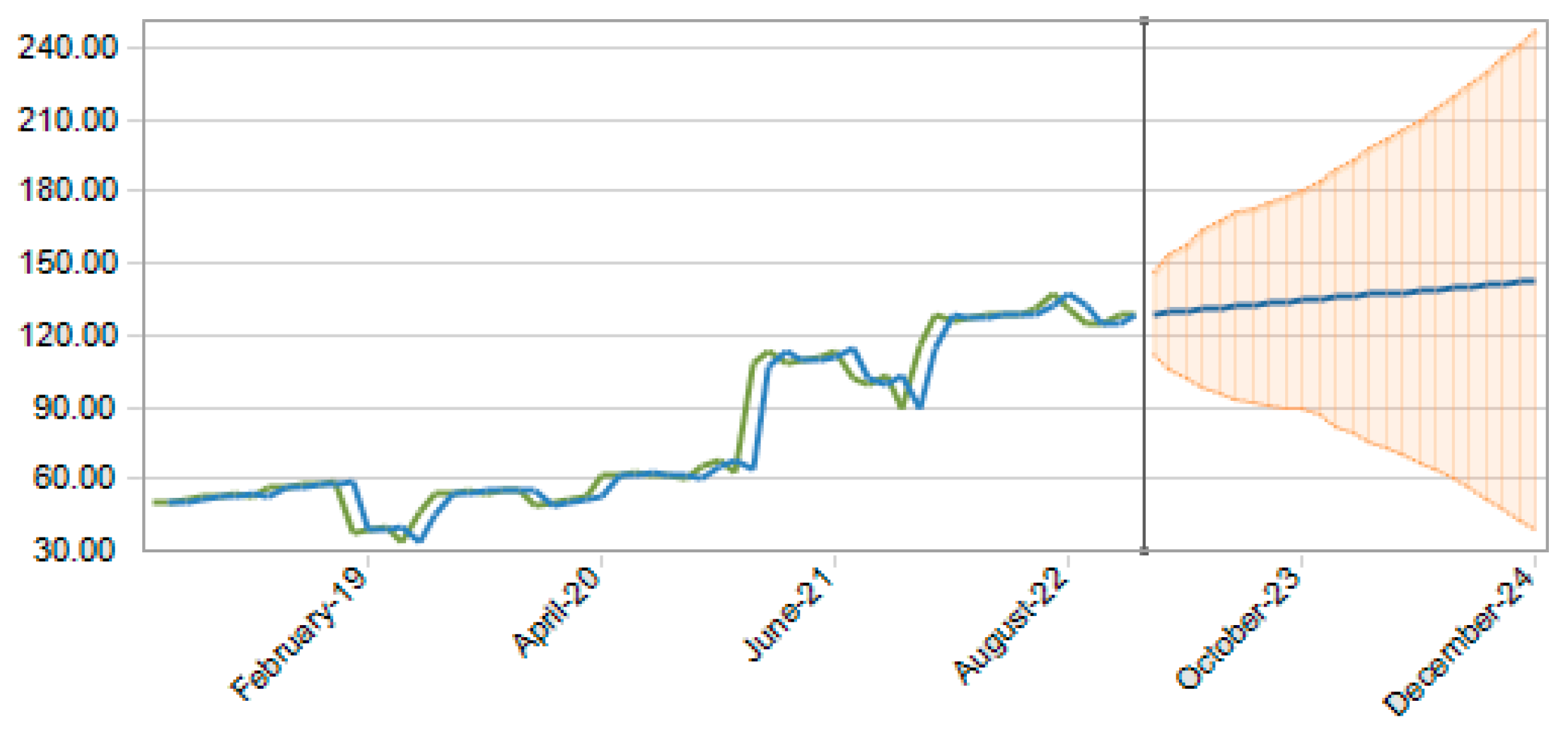
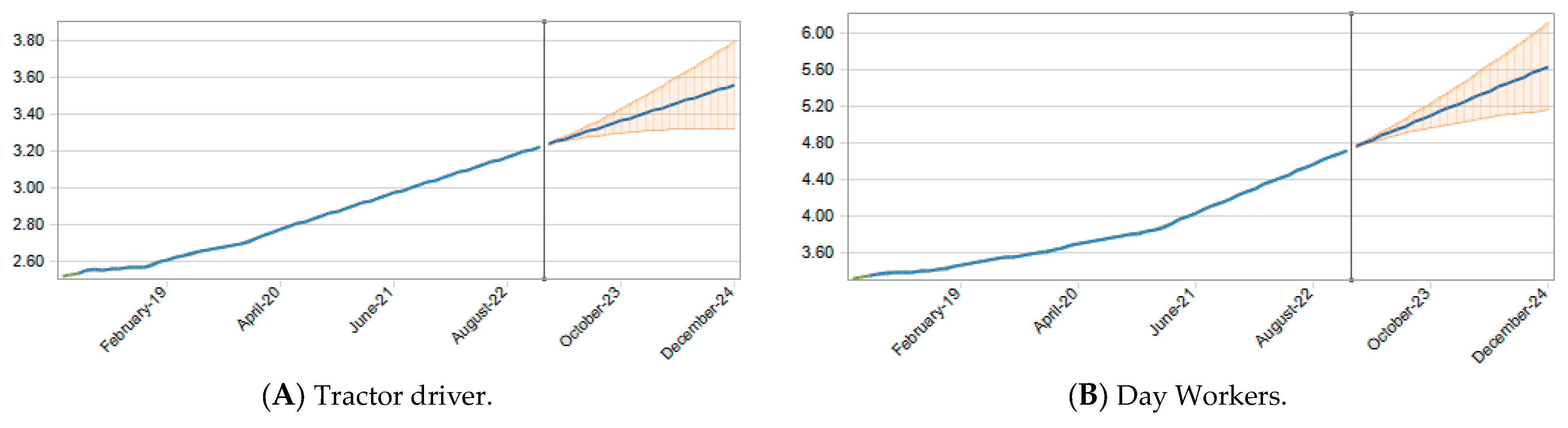
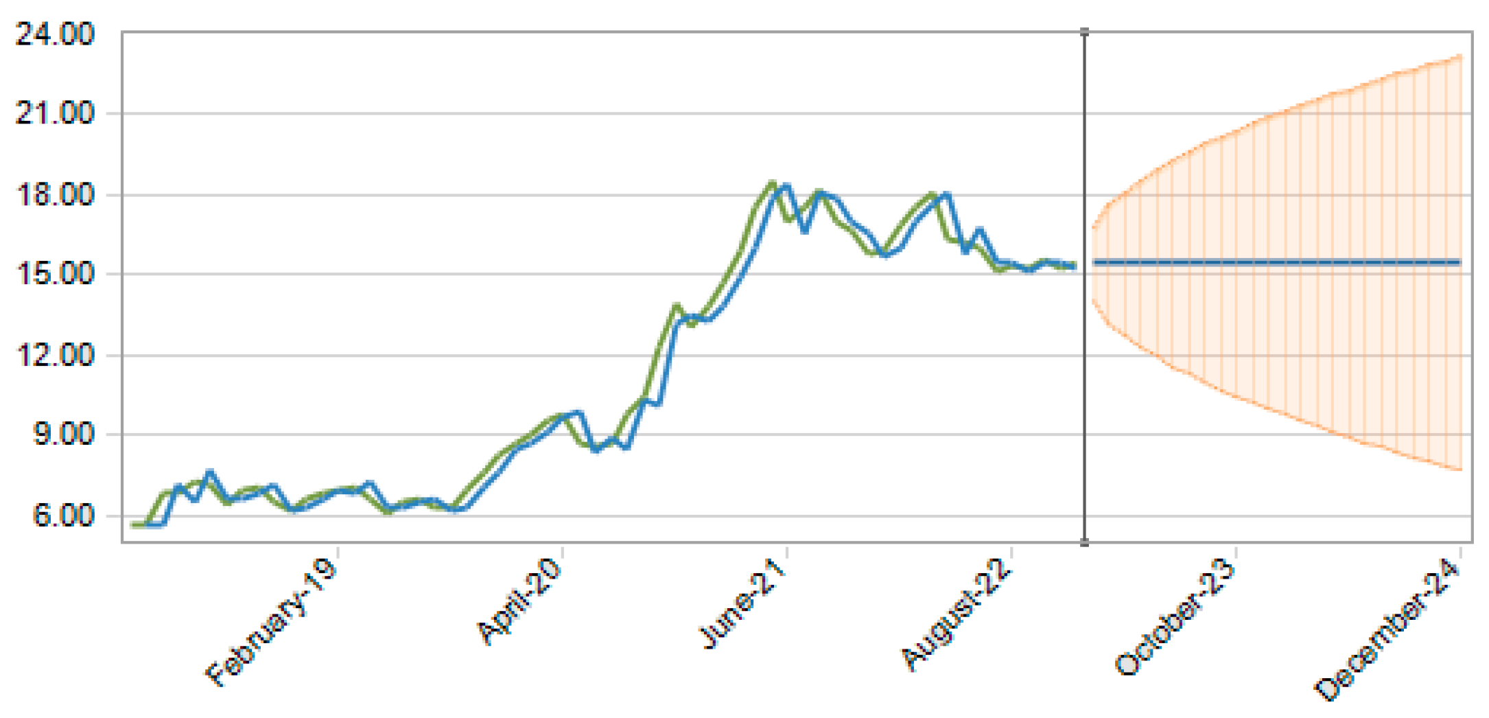
3.4. Time Series Forecasting Based on Historical Data

The urea fertilizer (Figure 3A) shows a trend of stability in its price for the next 24 months, while the NPK 05-25-25 fertilizer shows a downward trend (Figure 3B). It is possible to infer that the production cost of soybean planting is likely to decrease for the next two harvests, as the price of the NPK 05-25-25 fertilizer shows a strong correlation with the production cost of this crop. The stability in the price of urea for the next 24 months is due to the significant increase in the exchange rate in recent months, especially for the nitrogen component. It is important to note that the NPK 05-25-25 fertilizer uses 5% of this component in its formulation.

Among the models suggested by the software to forecast costs/ha for the next 24 months, DTN-S was able to capture the expected scenario for a near-term trend (730 days) for the cost/ton in Figure 3A, while ARIMA was used for Figure 3B. The blue line represents the price trend (3A) and (3B), and the orange area shows the range where this value can be found in the future trend.

The minimum cost/ha/soybean value for Figure 3A (urea fertilizer) was USD 33.90, and, for Figure 3B (NPK 05-25-25 fertilizer), it was USD 139.20. The average values were USD 58.04 and USD 288.02, and the maximum values were USD 120.15 and USD 602.62, with a standard deviation of USD 29.32 and USD 161.58, respectively. The purchasing power of rural producers to acquire one ton of fertilizers was reduced until July 2022, when a recovery trend began, observed in October [35]. As of April 2023, the price of one ton of NPK 05-25-25 fertilizer was USD 696.00, and the price of urea fertilizer was USD 718.00 [29]. These values are considered above the average predicted in this analysis. The difference between the maximum and minimum values presented in this analysis was significant.

Using the penalizing criteria of Akaike Information Criterion (AIC) and Bayesian Information Criterion (BIC), the best model for all the simulations performed was found. AIC acknowledges the existence of an unknown “true” model that describes the data and aims to select, among a group of evaluated models, the one that minimizes the Kullback–Leibler divergence (KL) and BIC, also known as Schwarz Information Criterion, is a criterion for model selection among a finite set of models. Models with lower BIC values are usually preferred [32].

Knowing that the model that best fits the series is the one with the lowest value, it can be concluded that the most suitable model for Figure 3B is the ARIMA (1, 1, 2) series. The model indicates an order of 1 for the AR component (Auto Regressive), an order of 1 for the 2 component (Integration or differencing), and the last 2 for the MA component (Moving Average). The values for AIC were 5.99 and for BIC were 6.10 * for Figure 3B, based on the lowest mean squared error. For the values presented in Figure 3A, the AIC was 3.32 and the BIC was 3.36 *.

The ARIMA model used for Figure 3A showed that the series has an insignificant auto-regressive (AR) component. This is due to the partial autocorrelations of the series, as evidenced by the ARIMA (0, 1, 1) model. However, even so, the autoregressive coefficients and the model coefficient weighted the behavior of the forecast, increasing the accuracy of this variable, thus demonstrating an appropriate model. Additionally, it can be observed that the Durbin–Watson (DW) statistic values, which indicate no first-order correlation, whether positive or negative, are equal to 2.0 for Figure 3A.

The TANS model for Figure 3B demonstrated that the series has a non-stationary stochastic process, as the statistical properties of at least one finite sequence of components differ from those of the sequence for at least one integer. In other words, a non-stationary stochastic process is one where the joint distribution of any set of variables changes if we change the variables over time. This is due to the partial correlations of the series, as evidenced by the ARIMA (1, 1, 2) model. Additionally, it can be observed from the Durbin–Watson (DW) statistic values that there is a first-order correlation, whether positive or negative, with values close to 2.0, as presented in Figure 3B.

The results presented in Figure 4 show the predicted values for dolomitic limestone corrective. The forecast indicates a stable scenario for the predicted 24 months. The minimum cost/ha/soybean/corn value was USD 14.80. The average value was equal to USD 25.29, and the maximum value reached USD 40.98, with a standard deviation of USD 8.02.

The current cost of dolomitic limestone corrective per hectare was USD 25.3 [29], which falls within the predicted average. The literature indicates that the costs associated with this soil corrective are mainly influenced by the freight rates during its transportation [67].

According to the Predictor, the best method with the lowest mean squared error chosen for all groups was the Damped Trend Non-Seasonal. Furthermore, it can be observed that the values of the Durbin–Watson statistic indicate no first-, second-, or third-order correlations, whether positive or negative. The analyzed material is essential for the cultivation of corn/soybean, as soil acidification is a concern in almost all countries with significant production of these crops, and its reversal contributes to water and nutrient exploitation, aiding the plant during periods of drought [68].

The results presented in Figure 5 show the estimated values of the Fungicide Trifloxystrobin Tebuconazole, which showed a strong relationship with the production costs of corn and soybean. The forecast indicates a scenario of price increase for the subsequent 24 months. This fungicide was the only agricultural pesticide with R² ≥ 0.70 for both crops and, thus, it can influence the increase in production costs for the studied crops.

The minimum cost per hectare for soybean/corn, as shown in Figure 5, was USD 25.43. The average cost was USD 28.92, and the maximum cost was USD 33.99, with a standard deviation of USD 2.64. According to [29], the cost at that moment of Trifloxystrobin Tebuconazole per hectare was USD 28.9, indicating that although there is a trend of price increase for this input over the next 24 months, the average cost remained within the estimated price by this forecast.

The statistical results conducted, according to the Predictor, showed that the best method with the lowest mean squared error chosen for all groups was DTN-S. This method is efficient for data with trends but without seasonality [32], which was the case in this analysis.

The estimated values for soybean seeds are presented in Figure 6. The results correspond to the values for both analyzed crops as dependent variables (corn/soybean). The forecast indicates a scenario of price increase for the next two years. The minimum cost per hectare for soybean seed was USD 34.29. The average cost was USD 79.93, and the maximum cost was USD 137.14, with a standard deviation of USD 33.28. The cost of soybean seed per hectare was USD 79.9 [53]. This value also falls within the predicted average produced by our model.

For the variable soybean seed, the most suitable method was DES. The results showed that the values of the DW statistic among all groups are close to 2.0.

Figure 7, presented below, shows the values and trends for the costs related to tractor drivers and day workers for both crops (corn/soybean). Figure 7A,B presents the trends for these variables, respectively. Both variables indicate an upward trend for the next 24 months.

The minimum cost per hectare for corn/soybean, as shown in Figure 7A, was USD 2.52, and, for Figure 7B, was USD 3.31. The average costs were USD 2.83 and USD 3.84, and the maximum costs were USD 3.23 and USD 4.72, with standard deviations of USD 0.22 and USD 0.42, respectively. The forecasted average values are aligned with the current values of USD 2.83 for tractor drivers and USD 3.84 for day workers [29].

The ARIMA models for Figure 7A,B demonstrated that the series has an insignificant autoregressive (AR) component. This is evident from the partial autocorrelations of the series, as shown in the ARIMA (0, 2, 0) model. The values of the DW statistic indicate that there is no first-order correlation, either positive or negative, with a value of 2.0 for Figure 7A and close to 2.0 for Figure 7B.

The results presented in Figure 8 are related to the price trend per corn bushel soon. However, it is evident that there is a stable price trend for corn per bushel in the coming 24 months.

The minimum price per bag for corn, as shown in Figure 8, was USD 5.66. The average price was USD 11.28, and the maximum price was USD 18.53, with a standard deviation of USD 4.52. The current price is USD 11.3, which falls within the predicted price range of this analysis (IEA, 2023).

Using the penalizing criteria of AIC and BIC, like Figure 3A, the ARIMA (1, 1, 1) model was found to be the best fit for the series. The AIC value was −0.65, and the BIC value was −5.58 *, based on the lowest mean squared error.

The statistical values for the MCS analysis conducted using the predictor, presented in the Figure 3, Figure 4, Figure 5, Figure 6, Figure 7 and Figure 8 (through a normal distribution), are summarized in

Table 4. Statistical analysis of the costs of corn/soybean and corn prices.

	Statistic DW			Theil’s U
	DTN-S	Arima (1, 1, 2)	DES	DTN-S	Arima (1, 1, 2)	DES	EM RMSE
NPKF (soybean)	1.92	1.92	1.97	0.96	0.96 *	0.97	9.9%
URF (soybean)	Tans	Arima (0, 1, 1)	Sed	Tans	Arima (0, 1, 1)	Sed	27.2%
	1.91	2.0	1.64	0.94	0.92 *	0.94
DLLC (soybean)	DTN-S	DMA	DES	DTN-S	DMA	DES	9.0%
	1.82	1.76	2.00	0.99 *	0.96	0.94
FUTT (soybean)	DES	DTN-S	SES	DES	DTN-S	SES	3.9%
	2.00	2.01	2.01	0.98 *	0.98	0.98
CORS	DES	DTN-S	SES	DES	DTN-S	SES	3.6%
	1.99	1.99	1.99	0.96 *	0.96	0.97
TRAC (corn/soybean)	DTN-S	Arima (0, 2, 0)	DES	DTN-S	Arima (0, 2, 0)	DES	6.0%
	1.70	2.00	1.70	0.99	0.99 *	0.99
Day (corn/soybean)	DTN-S	Arima (0, 2, 0)	DES	DTN-S	Arima (0, 2, 0)	DES	2.0%
	1.58	1.82	1.58	0.99	0.99 *	0.99
CORB (corn/soybean)	DTN-S	Arima (1, 1, 1)	DES	DTN-S	Arima (1, 1, 1)	DES	2.7%
	1.99	1.85	1.61	0.99	0.94 *	0.99

Statistical DW: Durbin–Watson; DTN-S: Damped Trend Non-Seasonal; DES: Double Exponential Smoothing; DMA: Double Moving Average; SES: Single Exponential Smoothing; NPKF: NPK 05-25-25 fertilizer; URF: Fertilizer Urea; DLLC: dolomitic limestone corrective; FUTT: fungicide trifloxystrobin tebuconazole; TRAC: tractor driver hours (h); DAI: daily worker hours (h); CORB: Corn bag. EM: Error Measure, RMSE: Root Mean Squared Error. * significant variable.

.

Thus, the results showed that inputs such as the NPK 05-25-25 fertilizer, Urea fertilizer, Dolomitic Limestone corrective, Trifloxystrobin Tebuconazole fungicide, soybean seed, day workers, tractor hours, and corn seed are relevant variables in estimating the production costs of corn and soybeans. Furthermore, cost forecasting using a Monte Carlo simulation provided a clear view of the expected costs for the next 24 months, enabling farmers to make strategic planning and resource allocation decisions.

The results also suggest a reduction in fertilizer costs, an increase in labor costs, soybean seed and fungicide costs, and stability in dolomitic limestone corrective costs in the near future (24 months). From the Monte Carlo simulation (MCS), the range of corn production costs is between USD 600.00 and USD 1150.00, with a level of certainty of 84.7%; and, of soybean production, costs between USD 260.00 and USD 420.00, with a level of certainty of 86.4%. These ranges of values demonstrate a high-cost risk level. Our findings also revealed that soybean profitability is higher than corn profitability based on the variables analyzed in this study.

The model predicted a trend of decreasing production costs for the crops in the 2023/24 and 2024/25 harvests if the costs of the most important inputs (i.e., fertilizers) decrease. On the other hand, the costs related to labor, soybean seed, and fungicides may show an upward trend, while the cost of dolomitic limestone corrective remains stable. Combined, these changes in the cost of inputs will increase the cost of crops and consequently their prices in the market.

Furthermore, with the expected increase in labor costs, it is essential to invest in training for workers, as well as considering possible mechanization to mitigate financial impacts. Additionally, a careful analysis of soybean seed varieties, adoption of integrated pest management, and strategic use of dolomitic limestone are relevant to deal with constantly changing costs. Adequate financial planning and the analysis of the feasibility of redirecting some of the cultivation areas to soybeans, given their higher profitability compared to corn, is also recommended. However, continuous monitoring of the production and market conditions should be made to make informed and sustainable decisions.

4. Conclusions

The model proposed here has shown accuracy in estimating future production prices of corn and soybeans. This makes it a useful tool to support pricing strategies under different production scenarios for these commodities, particularly in periods of significant market volatility and uncertainty. The model proposed forecasts prices more accurately, as it considers the variation in the costs of inputs that most significantly influence the costs of corn and soybean crops.

The model shows that production costs in the 2023/24 and 2024/25 harvests will depend mostly on the costs of labor, soybean seed, and fungicides, which may increase in this period. Several strategies and actions can be used to reduce these costs (e.g., changes in the cultivation areas, investment in mechanization, and digitalization of production processes). Furthermore, the results suggest that the profitability of soybean is higher than corn.

Understanding the factors that influence the costs of corn and soybeans inputs, as well as the behavior of price variability, is crucial for producers to make informed decisions on their crops. By doing so, it becomes possible to ensure the sustainability of agricultural production in competitive global markets.

Big Data applications can be particularly important in estimating future prices in so-called smart agriculture and they will be important to assist decision-makers and will influence the entire food supply chain [69]. More broadly, digital transformation, with its speed and scope, is revolutionizing agribusiness, modernizing production methods and profoundly changing the cost structure and risk management associated with crops [70]. However, these innovations also introduce new challenges, such as the need to manage additional costs and adapt to increasingly complex production dynamics [69].

In the context of the digital economy, crop cost risks are now influenced by new factors and variations. The increasing dependence on digital technologies implies costs for acquiring, maintaining, and updating software and hardware, making transactions more vulnerable to technological failures and obsolescence [69]. Furthermore, the volatility of costs has also increased, with machine learning techniques offering promises of more accurate specification, although these depend on the quality of the data and models used [70].

Looking ahead, digital transformation will continue to redefine the costs and risks associated with agricultural production. Farmers and businesses need to constantly adapt to new technologies to mitigate risks and take advantage of emerging opportunities [70]. However, this evolution can also accentuate technological inequalities, benefiting large producers to the detriment of smaller ones, which may face higher costs and challenges to compete [71]. Furthermore, digitalization can bring both sustainability benefits and new environmental risks, such as increased carbon footprint and challenges associated with cybersecurity, especially with the increasing interconnection of devices through the Internet of Things (IoT) [72,73].

This work stands out by applying MCS to model different cost scenarios, taking into account market volatility and the correlation between key variables. In this way, we not only address a gap identified in the literature but also offer a practical tool for economic and financial planning in agribusiness. This approach enables a more detailed and accurate analysis of the risks associated with production costs, offering managers a clearer view of potential cost variations, which is crucial for both operational and strategic decisions in such an uncertain environment.

However, it is important to recognize some limitations of this study. Firstly, the simulation model used is based on historical data and the precision of input parameter estimates, which can restrict the accuracy of forecasts in highly uncertain scenarios or in cases of abrupt changes in the market. Furthermore, the focus of this study was mainly on economic and cost variables, while other factors, such as climate change and government policies, which can also significantly impact production costs, were not addressed.

Thus, although our results are valuable for agribusiness decision-makers, further research is needed for a better understanding of the costs and prices of corn and soybean crops considering the current complexity of markets and modern production and business processes. Replicating the analysis in other countries with significant production of these crops, such as the United States and Argentina, would be also highly relevant.

Future research could expand the scope of this work by incorporating additional drivers of cost and price variability. Also, the influence of economic, environmental and political variables on production costs and competitiveness of corn and soybean crops can be studied. Furthermore, it would be relevant to investigate the use of other models, such as the fuzzy logic system, and artificial neural networks or hybrid models, which could complement Monte Carlo simulations, offering even more robust predictions in environments characterized by high uncertainty and volatility. Finally, a survey can be made to collect data and feedback from the stakeholders on these models and to support the design of effective and efficient policy recommendations.

Economic policies should, above all, aim to improve the efficiency and sustainability of agricultural production, strengthening producers’ capabilities to face higher uncertainty and volatility. For instance, training programs for rural producers in partnership with universities and other public and private organizations may increase farmers’ resilience to face market and environmental changes. Also, the use of renewable energies, the reduction of chemical inputs, and the use of precision agriculture techniques can contribute to reducing or dealing better with production and market variability.

References

1. Aragão, A.; Contini, E. O Agro no Brasil e no Mundo: Um Panorama do Período de 2000 a 2021; Embrapa: Brasilia, Brazil, 2022. [Google Scholar]
2. Meade, B.; Puricelli, E.; McBride, W.D.; Valdes, C.; Hoffman, L.; Foreman, L.; Dohlman, E. Corn and Soybean Production Costs and Export Competitiveness in Argentina, Brazil, and the United States; USDA Economic Information Bulletin; World Bank Group Agricuture: Washington, DC, USA, 2016. [Google Scholar]
3. Belik, W. Sustainability and Food Security after COVID-19: Relocalizing Food Systems? Agric. Econ. 2020, 8, 23. [Google Scholar] [CrossRef]
4. Amorim, F.R.; Silva, S.A.; Andrade, A.G.; Pigatto, G. Reflexo Pós-Pandemia Nos Preços das Ações de Três Grupos do Setor Sucroalcooleiro No Brasil. Navus 2021, 11, 1–19. [Google Scholar] [CrossRef]
5. Oliveira, S.C.D.; Amorim, F.R.D.; Barbosa, C.C.; Andrade, A.G.D.; Solfa, F.D.G. Effect of Production Costs on the Price per Ton of Sugarcane: The Case of Brazil. Int. J. Soc. Sci. Stud. 2022, 10, 15. [Google Scholar] [CrossRef]
6. Sun, Z.; Katchova, A.L.; Lee, S. Economic Perspective on the U.S. Agricultural Commodity Market for the 2022/23 Marketing Year; Department of Agricultural, Environmental and Development Economics: Columbus, OH, USA, 2023. [Google Scholar]
7. Grafton, M.; Manning, M. Establishing a Risk Profile for New Zealand Pastoral Farms. Agriculture 2017, 7, 81. [Google Scholar] [CrossRef]
8. Lips, M. Disproportionate Allocation of Indirect Costs at Individual-Farm Level Using Maximum Entropy. Entropy 2017, 19, 453. [Google Scholar] [CrossRef]
9. Gao, J.; McBride, W.D.; Ren, Z.; Ao, C.; Lei, G.; Gaiser, T.; Srivastava, A.K. A Fertilization Decision Model for Maize, Rice, and Soybean Based on Machine Learning and Swarm Intelligent Search Algorithms. Agronomy 2023, 13, 1400. [Google Scholar] [CrossRef]
10. Pitrova, J.; Krejčí, I.; Pilar, L.; Moulis, P.; Rydval, J.; Hlavatý, R.; Horáková, T.; Tichá, I. The Economic Impact of Diversification into Agritourism. Int. Food Agribus. Manag. Rev. 2020, 23, 713–734. [Google Scholar] [CrossRef]
11. Amorim, F.R.; Patino, M.T.O.; Bartmeyer, P.M.; Santos, D.F.L. Productivity and Profitability of the Sugarcane Production in the State of Sao Paulo, Brazil. Sugar Tech 2020, 22, 596–604. [Google Scholar] [CrossRef]
12. Goldsmith, P. Soybean Costs of Production. Afr. J. Food Agric. Nutr. Dev. 2020, 19, 15140–15144. [Google Scholar] [CrossRef]
13. Ishikawa-Ishiwata, Y.; Furuya, J. Fungicide Cost Reduction with Soybean Rust-Resistant Cultivars in Paraguay: A Supply and Demand Approach. Sustainability 2021, 13, 887. [Google Scholar] [CrossRef]
14. Huerta, A.I.H.; Martin, M.A. Soybean Production Costs: An Analysis of the United States, Brazil and Argentina. In Proceedings of the 2002 Annual Meeting, Long Beach, CA, USA, 28–31 July 2002. [Google Scholar]
15. Osaki, M.; Alves, L.R.A.; Lima, F.F.; Ribeiro, R.G.; Barros, G.S.C. Risks Associated with a Double-Cropping Production System—A Case Study in Southern Brazil. Sci. Agric. 2019, 76, 130–138. [Google Scholar] [CrossRef]
16. Arce, C.; Arias, D.; Caballero, J. Paraguay Agricultural Sector Risk Assessment; World Bank Group Agricuture: Washington, DC, USA, 2015. [Google Scholar]
17. Krah, K. Maize Price Variability, Land Use Change and Forest Loss: Evidence from Ghana. Land Use Policy 2023, 125, 106472. [Google Scholar] [CrossRef]
18. Wang, W.; Wei, L. Impacts of Agricultural Price Support Policy on Price Variability and Welfare: Evidence from China’s Soybean Market. Agric. Econ. 2021, 52, 3–17. [Google Scholar] [CrossRef]
19. De Oliveira Quadras, D.L.; Cavalcante, I.; Kück, M.; Mendes, L.G.; Frazzon, E.M. Machine Learning Applied to Logistics Decision Making: Improvements to the Soybean Seed Classification Process. Appl. Sci. 2023, 13, 10904. [Google Scholar] [CrossRef]
20. Koroteev, M.; Romanova, E.; Korovin, D.; Shevtsov, V.; Feklin, V.; Nikitin, P.; Makrushin, S.; Bublikov, K.V. Optimization of Food Industry Production Using the Monte Carlo Simulation Method: A Case Study of a Meat Processing Plant. Informatics 2022, 9, 5. [Google Scholar] [CrossRef]
21. Silva, S.A.; Abreu, P.H.C.; Amorim, F.R.; Santos, D.F.L. Application of Monte Carlo Simulation for Analysis of Costs and Economic Risks in a Banking Agency. IEEE Lat. Am. Trans. 2019, 17, 409–417. [Google Scholar] [CrossRef]
22. Oktoviany, P.; Knobloch, R.; Korn, R. A Machine Learning-Based Price State Prediction Model for Agricultural Commodities Using External Factors. Decis. Econ. Financ. 2021, 44, 1063–1085. [Google Scholar] [CrossRef]
23. Miura, M. Estimativa de Oferta e Demanda de Milho no Estado de São Paulo em 2022; Instituto de Economia Agrícola: São Paulo, Brazil, 2022; pp. 1–4. [Google Scholar]
24. SEADE. Valor da Produção Agrícola da Soja Ultrapassa o da Laranja em SP; Sistema Estadual de Análise de Dados: São Paulo, Brazil, 2022. [Google Scholar]
25. AGROSTAT—Estatisticas de Comércio Exterior do Agronegócio Brasileiro—2023; Ministério da Agricultura, Pecuária e Abastecimento: Brasilia, Brazil, 2023.
26. Gajić, T.; Petrović, M.D.; Blešić, I.; Radovanović, M.M.; Spasojević, A.; Sekulić, D.; Penić, M.; Demirović Bajrami, D.; Dubover, D.A. The Contribution of the Farm to Table Concept to the Sustainable Development of Agritourism Homesteads. Agriculture 2024, 14, 1314. [Google Scholar] [CrossRef]
27. Camargo, F.P.; Fredo, C.E.; Lago, C.S.; Ghobril, C.N.; Bini, D.L.; Angelo, J.A.; Miura, M.; Coelho, P.J.; Martins, V.A.; Nakama, L.M.; et al. Previsões e Estimativas das Safras Agrícolas do Estado de São Paulo, Levantamento Parcial, Ano Agrícola 2022/23 e Levantamento Final, Ano Agrícola 2021/2; Análises e Indicadores do Agronegócio: São Paulo, Brazil, 2023; pp. 1–20. [Google Scholar]
28. Moriasi, D.N.; Arnold, J.G.; Van Liew, M.W.; Bingner, R.L.; Harmel, R.D.; Veith, T.L. Model Evaluation Guidelines for Systematic Quantification of Accuracy in Watershed Simulations. Trans. ASABE 2007, 50, 885–900. [Google Scholar] [CrossRef]
29. São Paulo Banco de Dados; Instituto de Economia Agrícola-IEA: São Paulo, Brazil, 2023.
30. Ferraudo, A.S. Técnicas de Análise Multivariada: Uma Introdução. Apostila Técnica. Curso Análise Exploratória de Dados-Estatística Multivariada; Universidade Estadual Paulista: Jaboticabal, Brazil, 2014; 72p. [Google Scholar]
31. Hair, J.F.J.; Anderson, R.E.; Tatham, R.L.; Black, W.C. Análise Multivariada dos Dados; Bookman: Porto Alegre, Brazil, 2005. [Google Scholar]
32. EPM Information Development Team Oracle@Cloud. Como Trabalhar com Planejamento Preditivo no Smart View; Oracle Corporation: Austin, TX, USA, 2015; Available online: https://docs.oracle.com/cloud/help/pt_BR/pbcs_common/CSPPU/CSPPU.pdf (accessed on 2 April 2023).
33. Thompson, N.M.; Armstrong, S.D.; Roth, R.T.; Ruffatti, M.D.; Reeling, C.J. Short-run Net Returns to a Cereal Rye Cover Crop Mix in a Midwest Corn–Soybean Rotation. Agron. J. 2020, 112, 1068–1083. [Google Scholar] [CrossRef]
34. CEPEA. Custos Grãos; Centro de Estudos Avançados em Economia Aplicada: Piracicaba, Brazil, 2018. [Google Scholar]
35. CEPEA. Custos Grãos; Centro de Estudos Avançados em Economia Aplicada: Piracicaba, Brazil, 2019. [Google Scholar]
36. CEPEA. Custos Grãos; Centro de Estudos Avançados em Economia Aplicada: Piracicaba, Brazil, 2020. [Google Scholar]
37. CEPEA. Custos Grãos; Centro de Estudos Avançados em Economia Aplicada: Piracicaba, Brazil, 2021. [Google Scholar]
38. CEPEA. Custos Grãos; Centro de Estudos Avançados em Economia Aplicada: Piracicaba, Brazil, 2022. [Google Scholar]
39. Shadidi, B.; Najafi, G. Impact of Covid-19 on Biofuels Global Market and Their Utilization Necessity during Pandemic. Energy Equip. Syst. 2021, 9, 371–382. [Google Scholar] [CrossRef]
40. Lin, B.; Zhang, Y.Y. Impact of the COVID-19 Pandemic on Agricultural Exports. J. Integr. Agric. 2020, 19, 2937–2945. [Google Scholar] [CrossRef]
41. Facuri, F.G.; Ramos, M.R. Fatores de Influência Na Formação do Preço dos Herbicidas à Base de Glifosato No Brasil. Enciclopédia Biofesta 2019, 16, 882–894. [Google Scholar] [CrossRef]
42. Rabelo, C.G.; Souza, L.H.; Oliveira, F.G. Análise dos Custos de Produção de Silagem de Milho: Estudo de caso. Cad. Ciências Agrárias 2017, 9, 8–15. [Google Scholar]
43. Batista, A.; Lopes, A.C.V.; Costa, J.R.M. Gestão de Custos na Produção Agrícola: Um estudo na cultura da soja. In Proceedings of the XXIX Congresso Brasileiro de Custos, João Pessoa, Brazil, 16–18 November 2022. [Google Scholar]
44. Palma, A.A. Balanço de Pagamentos, Balança Comercial e Câmbio–Evolução Recente e Perspectivas; Instituto de Pesquisa Econômica Aplicada: Brasilia, Brazil, 2023. [Google Scholar]
45. Seidler, E.P.; Costa, N.L.; Almeida, M.; Coronel, D.A.; Santana, A.C. Formação de Preços do Milho em São Paulo e Suas Conexões Com o Mercado Interno e Internacional. Colóquio–Rev. Desenvolv. Reg. 2022, 19, 259–278. [Google Scholar]
46. Alves, L.R.A.; Costa, M.S.; Lima, F.F.; Souza, F.F.J.B.; Osaki, M.; Ribeiro, R.G. Diferenças nas Estruturas de Custos de Produção de Milho Convencional e Geneticamente Modificado no Brasil, na segunda safra: 2010/11, 2013/14 e 2014/15. Custos Agronegócio Online 2018, 14, 364–389. [Google Scholar]
47. Staugaitis, A.J.; Vaznonis, B. Short-Term Speculation Effects on Agricultural Commodity Returns and Volatility in the European Market Prior to and during the Pandemic. Agriculture 2022, 12, 623. [Google Scholar] [CrossRef]
48. Brum, A.L.; Baggio, D.K.; Souza, F.M.; Batista, G.; Schneider, I.N. Influência dos Fundos de Investimento Na Formação das Cotações do Milho Na Bolsa de Cereais de Chicago. Rev. Econ. Sociol. Rural 2023, 61, e251575. [Google Scholar] [CrossRef]
49. DIESSE. Redução do ICMS dos Combustíveis, Energia Elétrica, Transportes e Comunicação; Nota Técnica número 270; Departamento Intersindical de Estatística e Estudos Socioeconômicos: São Paulo, Brazil, 2022. [Google Scholar]
50. Olortegui, J.A.C.; Marçal, E.F.; Rocha, R.A.; Apolinário, H.C.F.; Teixeira, P.C.M. Avaliação de Áreas Agrícolas Através de Uma Abordagem de Opções Reais por Simulação de Monte Carlo Com Mínimos Quadrados Ordinários. Braz. J. Dev. 2021, 7, 118237–118255. [Google Scholar] [CrossRef]
51. Abreu, P.H.C.; Amorim, F.R. Gerenciamento Dos Riscos em Projetos de Software: Uma Aplicação da Simulação de Monte Carlo No Cronograma de Um Projeto. INFA 2017, 14, 53–71. [Google Scholar]
52. Joubert, F.; Pretorius, L. Using Monte Carlo Simulation to Create a Ranked Check List of Risks in a Portfolio of Railway Construction Projects. S. Afr. J. Ind. Eng. 2017, 28, 133–147. [Google Scholar] [CrossRef]
53. Custos-Soja-1997 a 2022; CONAB—Companhia Nacional de Abastecimento: Brasilia, Brazil, 2022.
54. Série Histórica-Custos-Milho 2a Safra-2005 a 2022; CONAB—Companhia Nacional de Abastecimento: Brasilia, Brazil, 2022.
55. Ventura, M.V.A.; Batista, H.R.F.; Bessa, M.M.; Pereira, L.S.; Costa, E.M.; Oliveira, M.H.R. Comparison of Conventional and Transgenic Soybean Production Costs in Different Regions in Brazil. RSD 2020, 9, e154973977. [Google Scholar] [CrossRef]
56. Münch, T.; Berg, M.; Mirschel, W.; Wieland, R.; Nendel, C. Considering Cost Accountancy Items in Crop Production Simulations Under Climate Change. Eur. J. Agron. 2014, 52, 57–68. [Google Scholar] [CrossRef]
57. Artuzo, F.D.; Foguesatto, C.R.; Souza, A.R.L.D.; Silva, L.X.D. Gestão de Custos na Produção de Milho e Soja. Rev. Bras. Gestão Negócios 2018, 20, 273–294. [Google Scholar]
58. Nóia Júnior, R.S.; Sentelhas, P.C. Soybean-Maize Succession in Brazil: Impacts of Sowing Dates on Climate Variability, Yields and Economic Profitability. Eur. J. Agron. 2019, 103, 140–151. [Google Scholar] [CrossRef]
59. Brookes, G.; Barfoot, P. GM Crop Technology Use 1996-2018: Farm Income and Production Impacts. GM Crops Food 2020, 11, 242–261. [Google Scholar] [CrossRef]
60. Baio, F.H.R.; Neves, D.C.; Souza, H.B.; Leal, A.J.F.; Leite, R.C.; Molin, J.P.; Silva, S.P. Variable Rate Spraying Application on Cotton Using an Electronic Flow Controller. Precis. Agric. 2018, 19, 912–928. [Google Scholar] [CrossRef]
61. Freitas, J.M.; Vaz, M.C.; Dutra, G.A.G.A.; Souza, J.L.; Rezende, C.F.A. Response of Corn Productivity to Mineral and Organomineral Fertilization. Res. Soc. Dev. 2021, 10, 26810514301. [Google Scholar]
62. Costa, F.G.; Caixeta Filho, J.V.; Arima, E. Influence of Transportation on the Use of the Land: Viabilization Potential of Soybean Production in Legal Amazon Due to the Development of the Transportation Infrastructure. Rev. Econ. Sociol. Rural. 2019, 39, 155–177. [Google Scholar]
63. Marchuk, S.; Tait, S.; Sinha, P.; Harris, P.; Antille, D.L.; McCabe, B.K. Biosolids-Derived Fertilisers: A Review of Challenges and Opportunities. Sci. Total Environ. 2023, 875, 162555. [Google Scholar] [CrossRef]
64. Smith, W.B.; Wilson, M.; Pagliari, P. Organomineral Fertilizers and Their Application to Field Crops. In Animal Manure: Production, Characteristics, Environmental Concerns, and Management; ASA Special Publications; Waldrip, H.M., Pagliari, P.H., He, Z., Eds.; American Society of Agronomy: Madison, WI, USA; Crop Science Society of America: Madison, WI, USA; Soil Science Society of America: Madison, WI, USA, 2020; pp. 229–243. ISBN 978-0-89118-371-6. [Google Scholar]
65. Van Lenteren, J.C.; Bolckmans, K.; Köhl, J.; Ravensberg, W.J.; Urbaneja, A. Biological Control Using Invertebrates and Microorganisms: Plenty of New Opportunities. BioControl 2018, 63, 39–59. [Google Scholar] [CrossRef]
66. Parra, J.R.P. Biological Control in Brazil: State of art and perspectives. Sci. Agric. 2023, 80, e20230080. [Google Scholar] [CrossRef]
67. CEPEA. Custos do Leite; Centro de Estudos Avançados em Economia Aplicada: Piracicaba, Brazil, 2018. [Google Scholar]
68. Beerling, D.J.; Leake, J.R.; Long, S.P.; Scholes, J.D.; Ton, J.; Nelson, P.N.; Bird, M.; Kantzas, E.; Taylor, L.L.; Sarkar, B.; et al. Farming with Crops and Rocks to Address Global Climate, Food and Soil Security. Nat. Plants 2018, 4, 138–147. [Google Scholar] [CrossRef] [PubMed]
69. Wolfert, S.; Ge, L.; Verdouw, C.; Bogaardt, M. Big Data in Smart Farming—A Review. Agric. Syst. 2017, 153, 69–80. [Google Scholar] [CrossRef]
70. Klerkx, L.; Rose, D. Dealing with the Game-Changing Technologies of Agriculture 4.0: How Do We Manage Diversity and Responsibility in Food System Transition Pathways? Glob. Food Secur. 2020, 24, 100347. [Google Scholar] [CrossRef]
71. Rose, D.C.; Chilvers, J. Agriculture 4.0: Broadening Responsible Innovation in an Era of Smart Farming. Front. Sustain. Food Syst. 2018, 2, 87. [Google Scholar] [CrossRef]
72. Sundmaeker, H.V.C.; Verdouw, C.; Wolfert, S.; Freire, L.P. Internet of Food and Farm 2020. In Digitising the Industry-Internet of Things Connecting the Physical, Digital and Virtual Worlds; River Publishers: Alborg, Denmark, 2016; Volume 1, pp. 129–151. ISBN 978-1-00-333796-6. [Google Scholar]
73. Kamilaris, A.; Kartakoullis, A.; Prenafeta-Boldú, F.X. A Review on the Practice of Big Data Analysis in Agriculture. Comput. Electron. Agric. 2017, 143, 23–37. [Google Scholar] [CrossRef]
Figure 1. Frequency graph of total cost soy/hectare.
Applsci 14 08030 g001
Figure 2. Frequency graph of total cost corn/hectare.
Applsci 14 08030 g002
Figure 3. Price trends for the next 24 months of the variables (green line: historical data, blue line: fitted and forecast; orange area: forecast range with lower and upper bounds of 2.5% and 97.5%, respectively).
Applsci 14 08030 g003
Figure 4. Price trend for the next 24 months of the dolomitic limestone corrective (green line: historical data, blue line: fitted and forecast; orange area: forecast range with lower and upper bounds of 2.5% and 97.5%, respectively).
Applsci 14 08030 g004
Figure 5. Price trend for the next 24 months of the fungicide variable Trifloxystrobin Tebuconzole (green line: historical data, blue line: fitted and forecast; orange area: forecast range with lower and upper bounds of 2.5% and 97.5%, respectively).
Applsci 14 08030 g005
Figure 6. Price trend for the next 24 months of the variable soybean seed (green line: historical data, blue line: fitted and forecast; orange area: forecast range with lower and upper bounds of 2.5% and 97.5%, respectively).
Applsci 14 08030 g006
Figure 7. Price trend for the next 24 months of the tractor driver labor costs (A) and day workers labor costs (B) (green line: historical data; blue line: fitted and forecast; orange area: forecast range with lower and upper bounds of 2.5% and 97.5%, respectively).
Applsci 14 08030 g007
Figure 8. Price trend for the next 24 months of corn per bag (green line: historical data; blue line: fitted and forecast; orange area: forecast range with lower and upper bounds of 2.5% and 97.5%, respectively).
Applsci 14 08030 g008