
AEA-RDCP: An Optimized Real-Time Algorithm for Sea Fog Intensity and Visibility Estimation


Abstract
1. Introduction
2. Literature Review
2.1. Visibility Estimation Studies
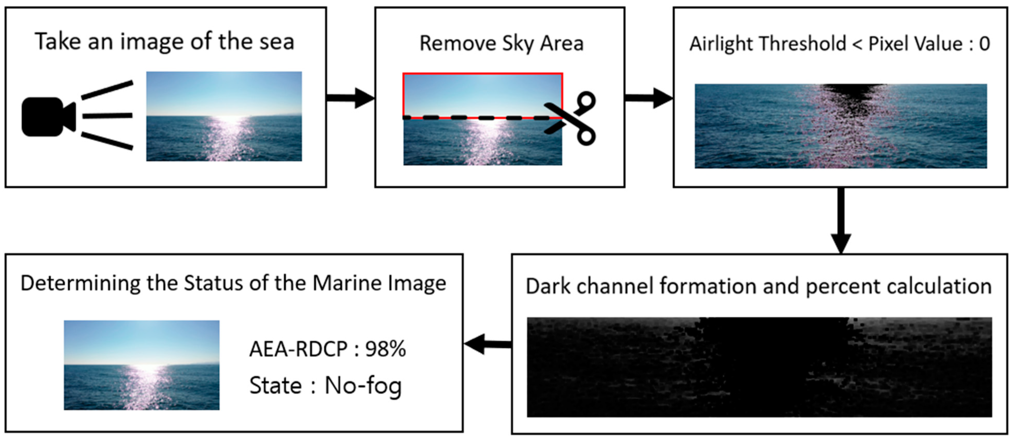
- Generation of the DC Image: Creating the DC image using the minimum values per channel from local patches;
- Estimation of Atmospheric Light: Calculating the atmospheric light value using the brightest pixels in the DC image;
- Estimation of the Transmission Map: Calculating an initial transmission map, then refining it to obtain the final transmission map;
- Calculation of the Restored Image: Using the transmission map and atmospheric light value to restore the original image.
2.2. Image-Based Sea Fog Strength Measurement Algorithm Using DC (RDCP)
2.3. Effects of Atmospheric Light on Visibility Estimation
3. Approximating and Eliminating the Airlight—Reduced DCP (AEA-RDCP)
3.1. AEA-RDCP
3.2. Example of Setting and Applying Ambient Light Estimation Thresholds
- I(x) is the observed pixel value of the image;
- J(x) is the actual pixel value of the scene without fog;
- t(x) is the transmission map, which is related to the depth of the scene and indicates how much the pixel has been attenuated by atmospheric particles;
- A is the atmospheric light, representing the brightest part of the scene;
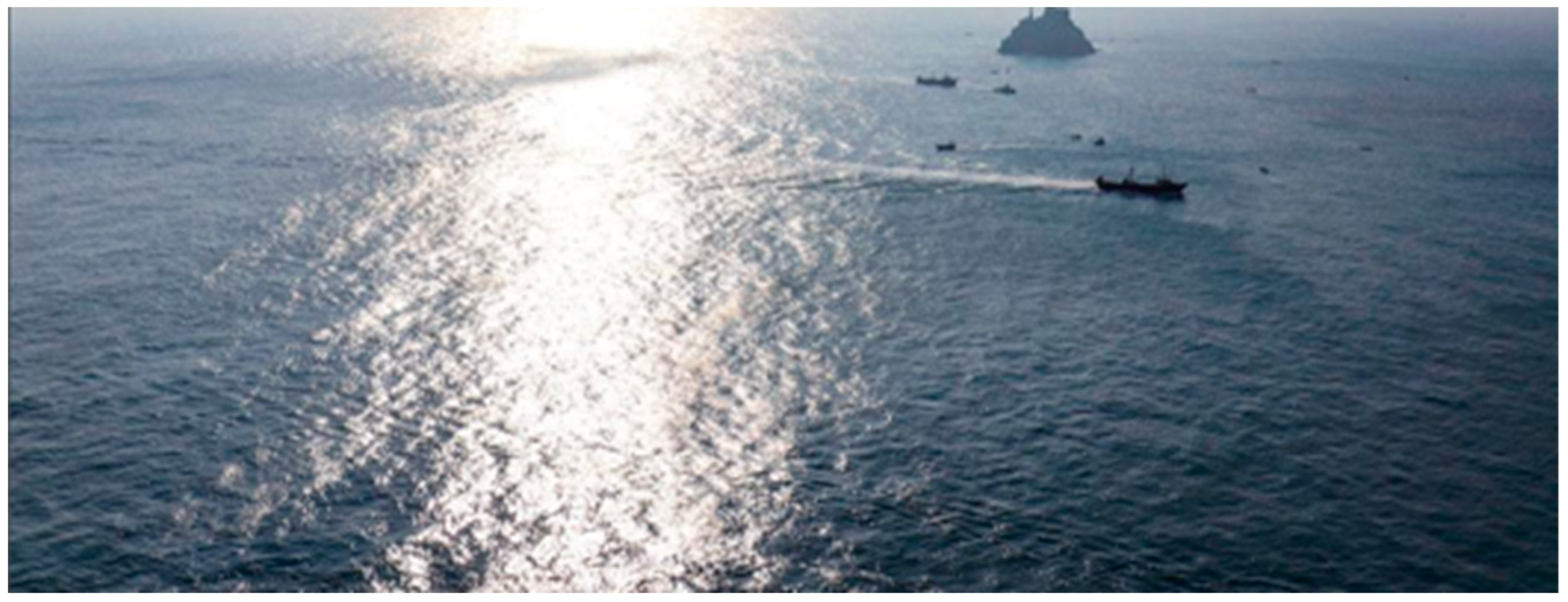
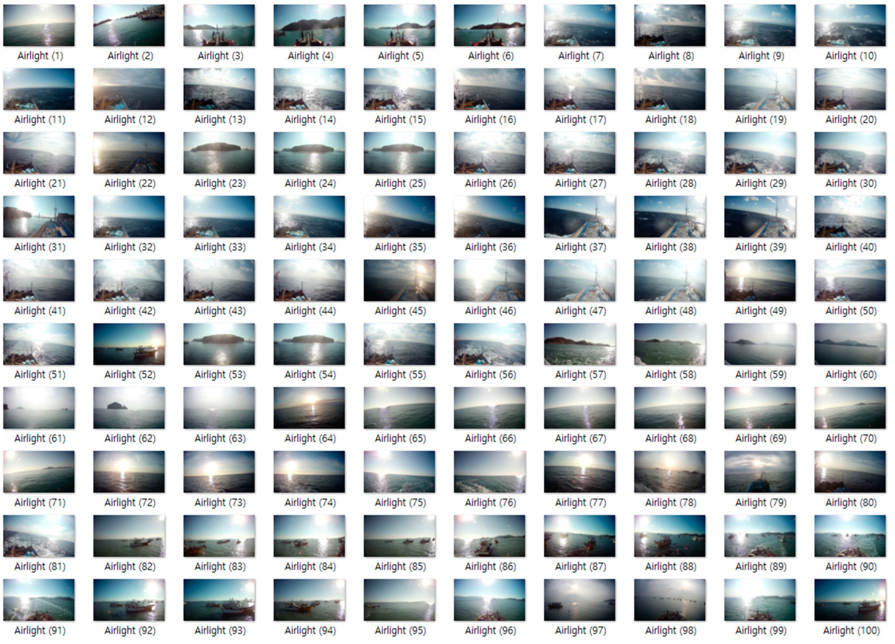
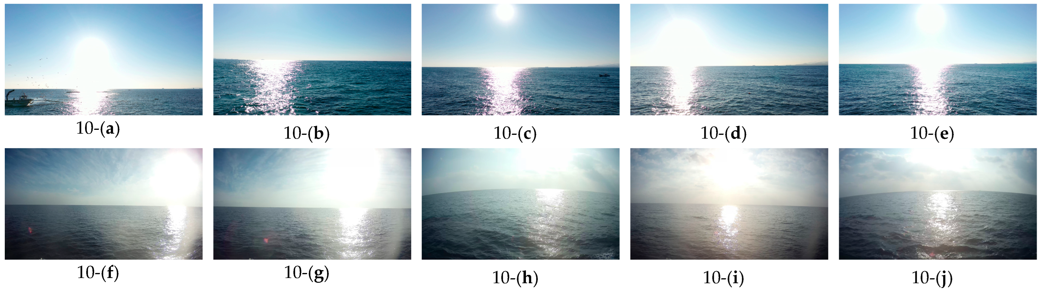
- Dataset Selection: A dataset of 100 images with a resolution of 3840 × 2160 pixels was selected for threshold estimation, as illustrated in Figure 6. These images were taken under strong sunlight conditions and were carefully curated from the AI Hub dataset, focusing on days with abundant sunlight across various times of the day [34].
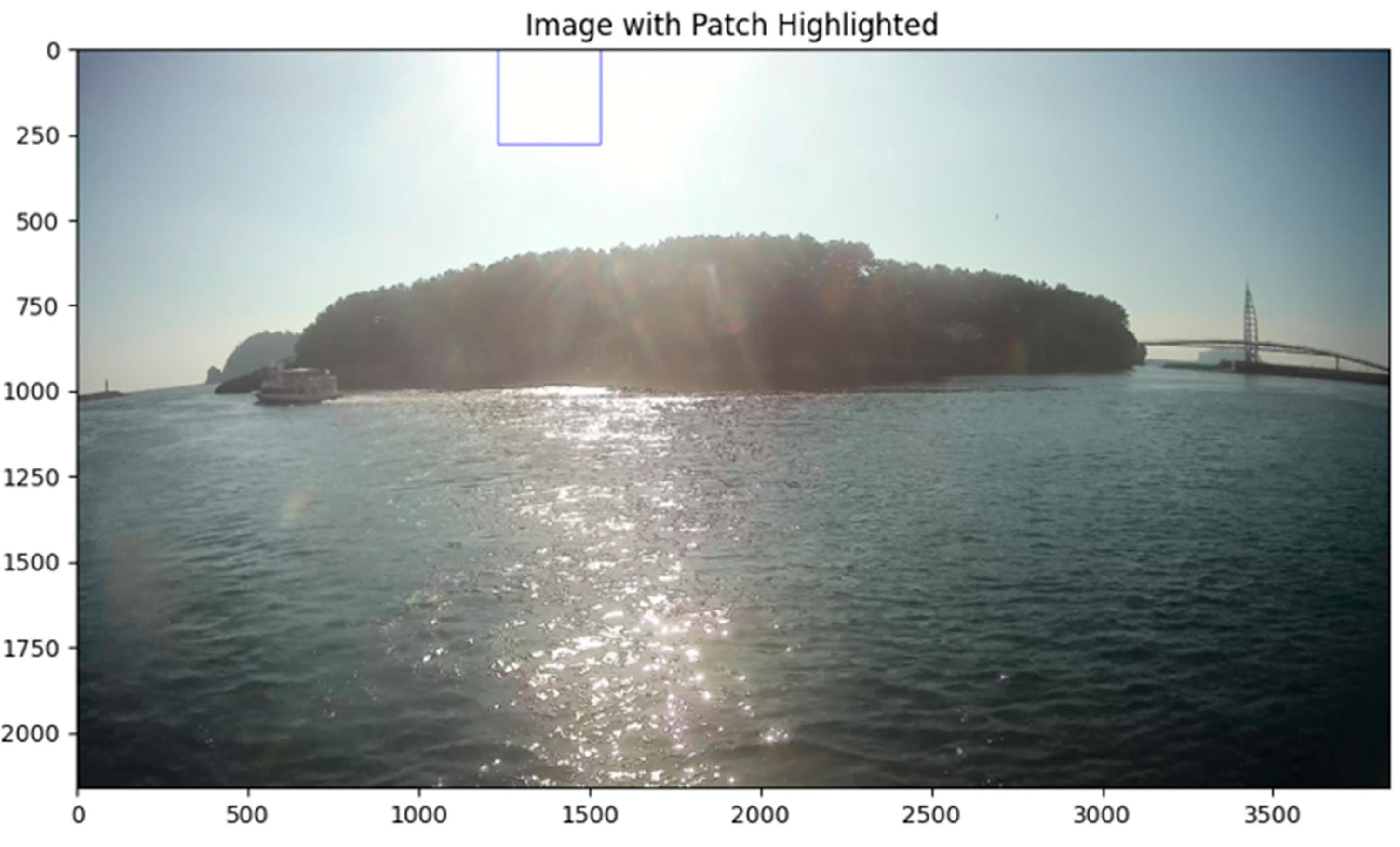
- DC Image Creation: For each image, the minimum value among the R, G, and B channels of every pixel was chosen to generate the DC image, which captures the impact of fog.
- Brightest Pixel Selection: The top 0.1% brightest pixels in the DC image were identified.
- Patch Extraction: Patches of 301 × 301 pixels surrounding these brightest pixels were extracted to ensure accurate estimation by excluding pixels affected by atmospheric light.
- Threshold Calculation: The average values of the R, G, and B channels within these patches were calculated [35]. These averages were then used as the threshold for atmospheric light estimation.
| Algorithm 1. Process of obtaining the threshold value of the ambient light estimation pixel. |
| 1. Prepare Sunlight Images: 100 images - Load up to 100 images from the image folder. 2. Generate Dark Channel Image: For each image do - Select the minimum value among the R, G, B channels for each pixel to create the dark channel image. - Apply erosion operation to the dark channel image to obtain the final dark channel image. 3. Select the brightest pixel among the top 0.1% pixels in the Dark Channel image: - Select the top 0.1% brightest pixels in the dark channel image. - Find the brightest pixel among them. 4. Extract a patch around the brightest pixel and calculate the average R, G, B values in this patch: - Extract a patch of fixed size around the coordinates of the brightest pixel. - Calculate the average R, G, B values of all pixels in this patch. 5. Determine the calculated average values as the threshold for estimating atmospheric light pixels: - Use the calculated average R, G, B values as the atmospheric light estimate. |
4. Experiments and Evaluations
4.1. Experimental Dataset
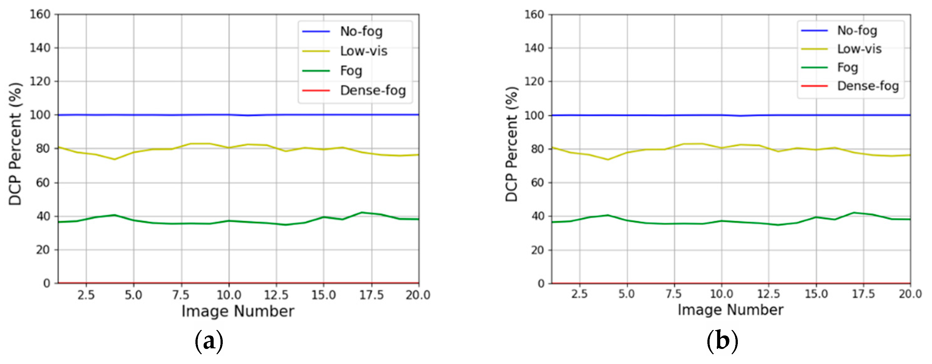
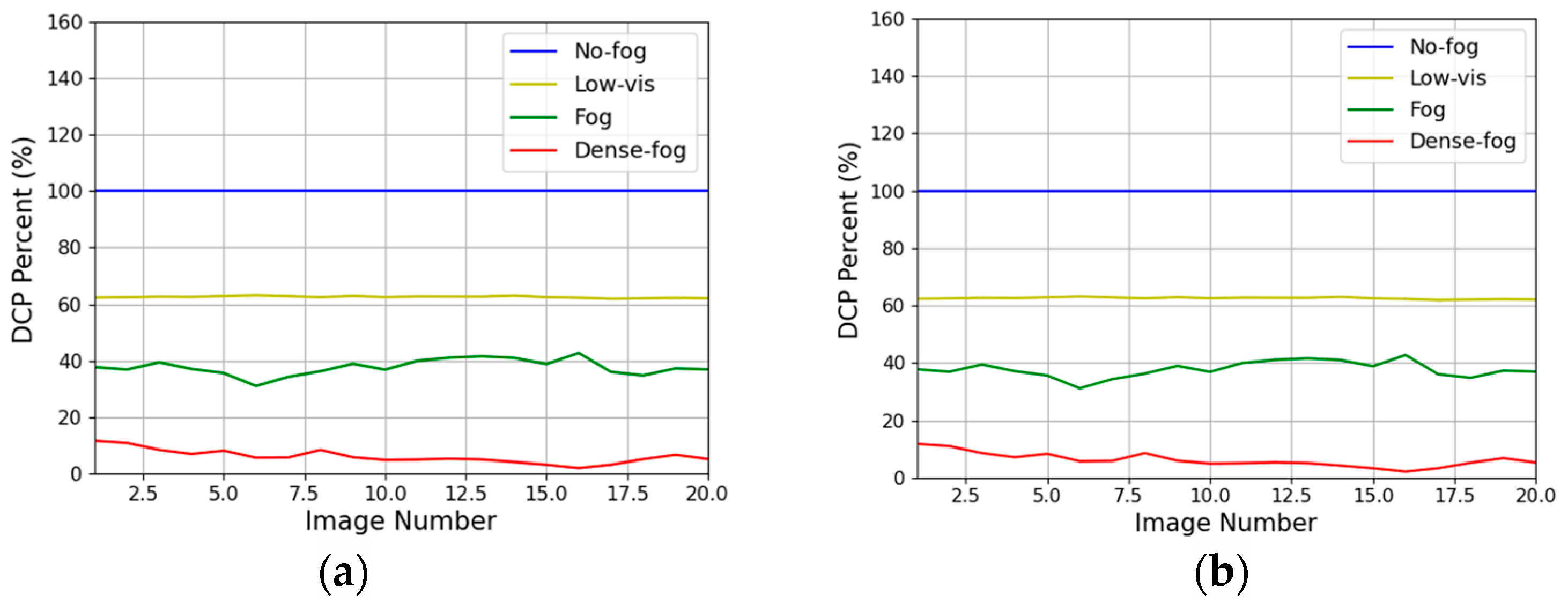
4.2. Dataset without the Influence of Atmospheric Light: Performance Comparison and Evaluation with RDCP
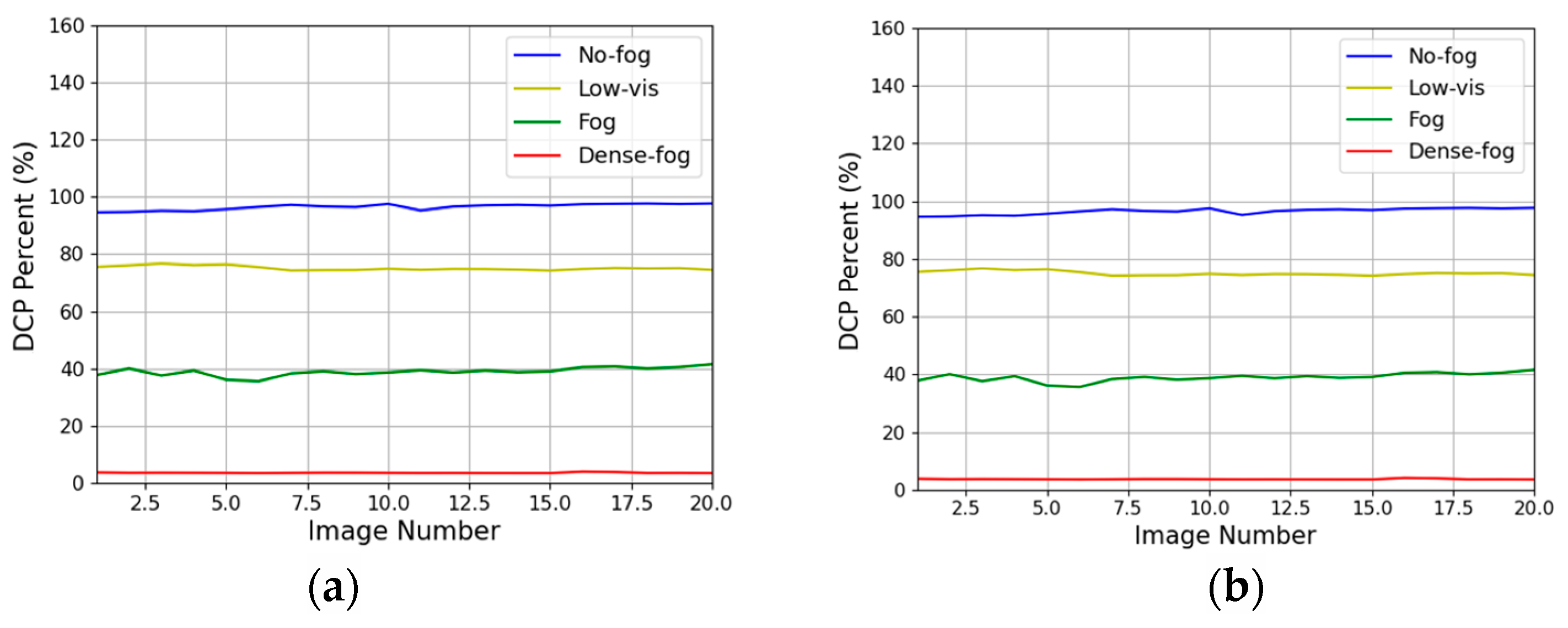
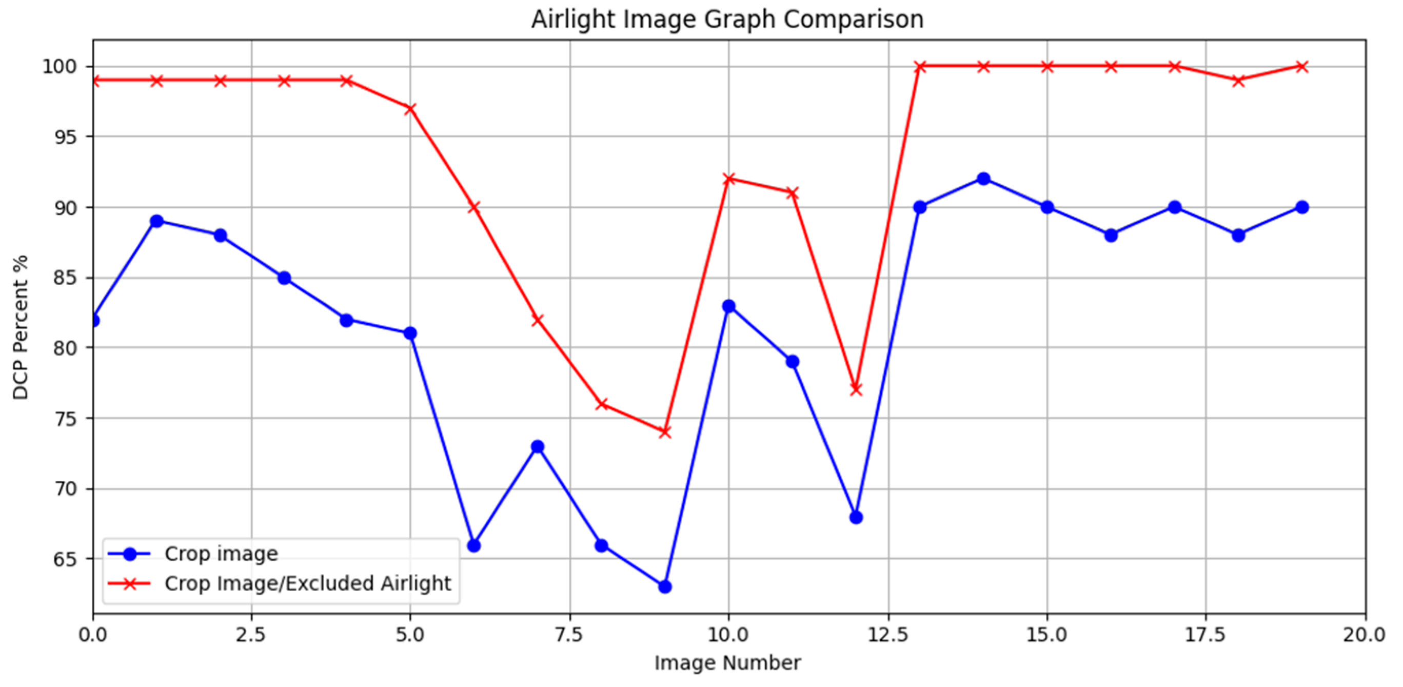
4.3. Dataset Affected by Atmospheric Light: AEA-RDCP Performance Evaluation
4.4. Visibility Estimation
5. Conclusions
Author Contributions
Funding
Institutional Review Board Statement
Informed Consent Statement
Data Availability Statement
Conflicts of Interest
References
- Koračin, D.; Dorman, C.E.; Mejia, J.; McEvoy, D. Marine Fog: Challenges and Advancements in Observations, Modeling, and Forecasting; Springer: Berlin/Heidelberg, Germany, 2024. [Google Scholar]
- Jeon, H.-K.; Kim, S.; Edwin, J.; Yang, C.-S. Sea Fog Identification from GOCI Images Using CNN Transfer Learning Models. Electronics 2020, 9, 311. [Google Scholar] [CrossRef]
- Shao, N.; Lu, C.; Jia, X.; Wang, Y.; Li, Y.; Yin, Y.; Zhu, B.; Zhao, T.; Liu, D.; Niu, S.; et al. Radiation fog properties in two consecutive events under polluted and clean conditions in the Yangtze River Delta, China: A simulation study. Atmos. Chem. Phys. 2023, 23, 9873–9890. [Google Scholar] [CrossRef]
- Wang, Y.; Lu, C.; Niu, S.; Lv, J.; Jia, X.; Xu, X.; Xue, Y.; Zhu, L.; Yan, S. Diverse dispersion effects and parameterization of relative dispersion in urban fog in eastern China. J. Geophys. Res. Atmos. 2023, 128, e2022JD037514. [Google Scholar] [CrossRef]
- Yang, D.; Zhu, Z.; Ge, H.; Qiu, H.; Wang, H.; Xu, C. A Lightweight Neural Network for the Real-Time Dehazing of Tidal Flat UAV Images Using a Contrastive Learning Strategy. Drones 2024, 8, 314. [Google Scholar] [CrossRef]
- Liang, C.W.; Chang, C.C.; Liang, J.J. The impacts of air quality and secondary organic aerosols formation on traffic accidents in heavy fog–Haze weather. Heliyon 2023, 9, e14631. [Google Scholar] [CrossRef] [PubMed]
- World Meteorological Organization. Guide to Meteorological Instruments and Methods of Observation; World Meteorological Organization: Geneva, Switzerland, 2017; p. 1177. [Google Scholar]
- Korea Open MET Data Portal. Available online: https://data.kma.go.kr/climate/fog/selectFogChart.do?pgmNo=706 (accessed on 25 November 2023).
- Lee, H.K.; Shu, M.S. A Comparative Study on the Visibility Characteristics of Naked-Eye. Atmosphere 2018, 28, 69–83. [Google Scholar]
- The Korea Economic Daily: Ongjin County Council Urged the Ministry of Oceans and Fisheries to Ease the Visibility-Related Regulations. 18 October 2021. Available online: https://www.hankyung.com/society/article/202110280324Y (accessed on 25 November 2023).
- Hwang, S.-H.; Park, S.-K.; Park, S.-H.; Kwon, K.-W.; Im, T.-H. RDCP: A Real Time Sea Fog Intensity and Visibility Estimation Algorithm. J. Mar. Sci. Eng. 2024, 12, 53. [Google Scholar] [CrossRef]
- Wang, S.; Wang, S.; Jiang, Y.; Zhu, H. Discerning Reality through Haze: An Image Dehazing Network Based on Multi-Feature Fusion. Appl. Sci. 2024, 14, 3243. [Google Scholar] [CrossRef]
- He, K.; Sun, J.; Tang, X. Single image haze removal using dark channel prior. IEEE Trans. Pattern Anal. Mach. Intell. 2010, 33, 2341–2353. [Google Scholar]
- Narasimhan, S.G.; Nayar, S.K. Contrast Restoration of Weather Degraded Images. IEEE Trans. Pattern Anal. Mach. Intell. 2003, 25, 713–724. [Google Scholar] [CrossRef]
- Wang, Y.; Qiu, Z.; Zhao, D.; Ali, M.A.; Hu, C.; Zhang, Y.; Liao, K. Automatic Detection of Daytime Sea Fog Based on Supervised Classification Techniques for FY-3D Satellite. Remote Sens. 2023, 15, 2283. [Google Scholar] [CrossRef]
- Narendra, K.; Chandrasekaran, M. Performance evaluation of various dehazing techniques for visual surveillance applications. Signal Image Video Process. 2016, 10, 267–274. [Google Scholar]
- Tarel, J.-P.; Hautière, N. Fast visibility restoration from a single color or gray level image. In Proceedings of the IEEE International Conference on Computer Vision (ICCV), Kyoto, Japan, 29 September–2 October 2009; pp. 2201–2208. [Google Scholar]
- Chiang, J.Y.; Chen, Y.-C. Underwater image enhancement by wavelength compensation and dehazing. IEEE Trans. Image Process. 2012, 21, 1755–1769. [Google Scholar] [CrossRef]
- Li, B.; Peng, X.; Wang, Z.; Xu, J.; Feng, D. Aod-Net: All-in-One Dehazing Network. In Proceedings of the IEEE International Conference on Computer Vision (ICCV), Venice, Italy, 22–29 October 2017; pp. 4770–4778. [Google Scholar]
- Zhu, Q.; Mai, J.; Shao, L. A fast single image haze removal algorithm using color attenuation prior. IEEE Trans. Image Process. 2015, 24, 3522–3533. [Google Scholar]
- Outay, F.; Taha, B.; Chaabani, H.; Kamoun, F.; Werghi, N.; Yasar, A. Estimating ambient visibility in the presence of fog: A deep convolutional neural network approach. Pers. Ubiquitous Comput. 2021, 25, 51–62. [Google Scholar] [CrossRef]
- Bae, T.W.; Han, J.H.; Kim, K.J.; Kim, Y.T. Coastal Visibility Distance Estimation Using Dark Channel Prior and Distance Map Under Sea-Fog: Korean Peninsula Case. Sensors 2019, 19, 4432. [Google Scholar] [CrossRef] [PubMed]
- Yang, L. Comprehensive Visibility Indicator Algorithm for Adaptable Speed Limit Control in Intelligent Transportation Systems. Ph.D. Thesis, University of Guelph, Guelph, ON, Canada, 2018. [Google Scholar]
- Ryu, E.J.; Lee, H.C.; Cho, S.Y.; Kwon, K.W.; Im, T.H. Sea Fog Level Estimation based on Maritime Digital Image for Protection of Aids to Navigation. J. Korean Soc. Internet Inf. 2021, 22, 25–32. [Google Scholar]
- Jeon, H.S.; Park, S.H.; Im, T.H. Grid-Based Low Computation Image Processing Algorithm of Maritime Object Detection for Navigation Aids. Electronics 2023, 12, 2002. [Google Scholar] [CrossRef]
- Tan, R.T. Visibility in Bad Weather from a Single Image. In Proceedings of the IEEE Conference on Computer Vision and Pattern Recognition (CVPR), Anchorage, AK, USA, 23–28 June 2008; pp. 1–8. [Google Scholar]
- Meng, G.; Wang, Y.; Duan, J.; Pan, C.; Yang, X. Efficient Image Dehazing with Boundary Constraint and Contextual Regularization. In Proceedings of the IEEE International Conference on Computer Vision (ICCV), Sydney, Australia, 1–8 December 2013; pp. 617–624. [Google Scholar]
- Li, W.; Liu, Y.; Ou, X.; Wu, J.; Guo, L. Enhancing Image Clarity: A Non-Local Self-Similarity Prior Approach for a Robust Dehazing Algorithm. Electronics 2023, 12, 3693. [Google Scholar] [CrossRef]
- Liu, S.; Li, Y.; Li, H.; Wang, B.; Wu, Y.; Zhang, Z. Visual Image Dehazing Using Polarimetric Atmospheric Light Estimation. Appl. Sci. 2023, 13, 10909. [Google Scholar] [CrossRef]
- Fattal, R. Single image dehazing. ACM Trans. Graph. (TOG) 2008, 27, 1–9. [Google Scholar] [CrossRef]
- Ancuti, C.O.; Ancuti, C.; De Vleeschouwer, C. Effective Local Airlight Estimation for Image Dehazing. In Proceedings of the 2018 25th IEEE International Conference on Image Processing (ICIP), Athens, Greece, 7–10 October 2018; pp. 2850–2854. [Google Scholar] [CrossRef]
- Ancuti, C.; Ancuti, C.O.; De Vleeschouwer, C.; Bovik, A.C. Day and Night-Time Dehazing by Local Airlight Estimation. IEEE Trans. Image Process. 2020, 29, 6264–6275. [Google Scholar] [CrossRef] [PubMed]
- Berman, D.; Avidan, S. Non-Local Image Dehazing. In Proceedings of the IEEE Conference on Computer Vision and Pattern Recognition (CVPR), Las Vegas, NV, USA, 27–30 June 2016; pp. 1674–1682. [Google Scholar]
- AI Hub. Available online: https://aihub.or.kr/aihubdata/data/view.do?currMenu=&topMenu=&aihubDataSe=data&dataSetSn=175 (accessed on 8 July 2023).
- Yang, S.; Liang, H.; Wang, Y.; Cai, H.; Chen, X. Image Inpainting Based on Multi-Patch Match with Adaptive Size. Appl. Sci. 2020, 10, 4921. [Google Scholar] [CrossRef]
- An, J.; Son, K.; Jung, K.; Kim, S.; Lee, Y.; Song, S.; Joo, J. Enhancement of Marine Lantern’s Visibility under High Haze Using AI Camera and Sensor-Based Control System. Micromachines 2023, 14, 342. [Google Scholar] [CrossRef] [PubMed]


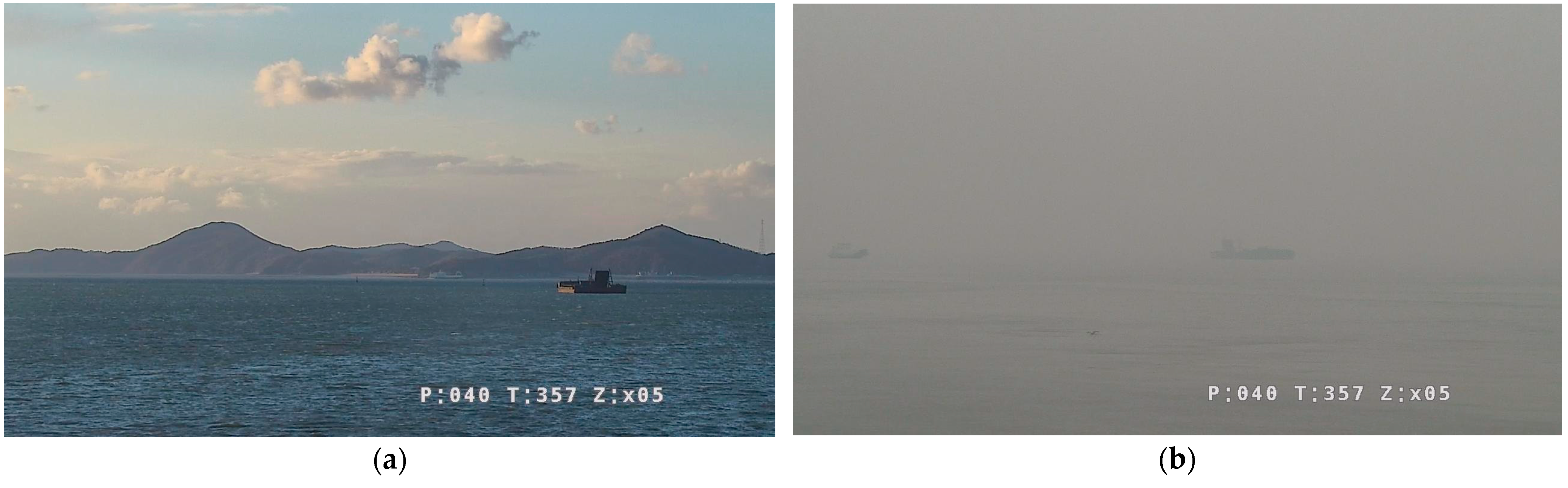
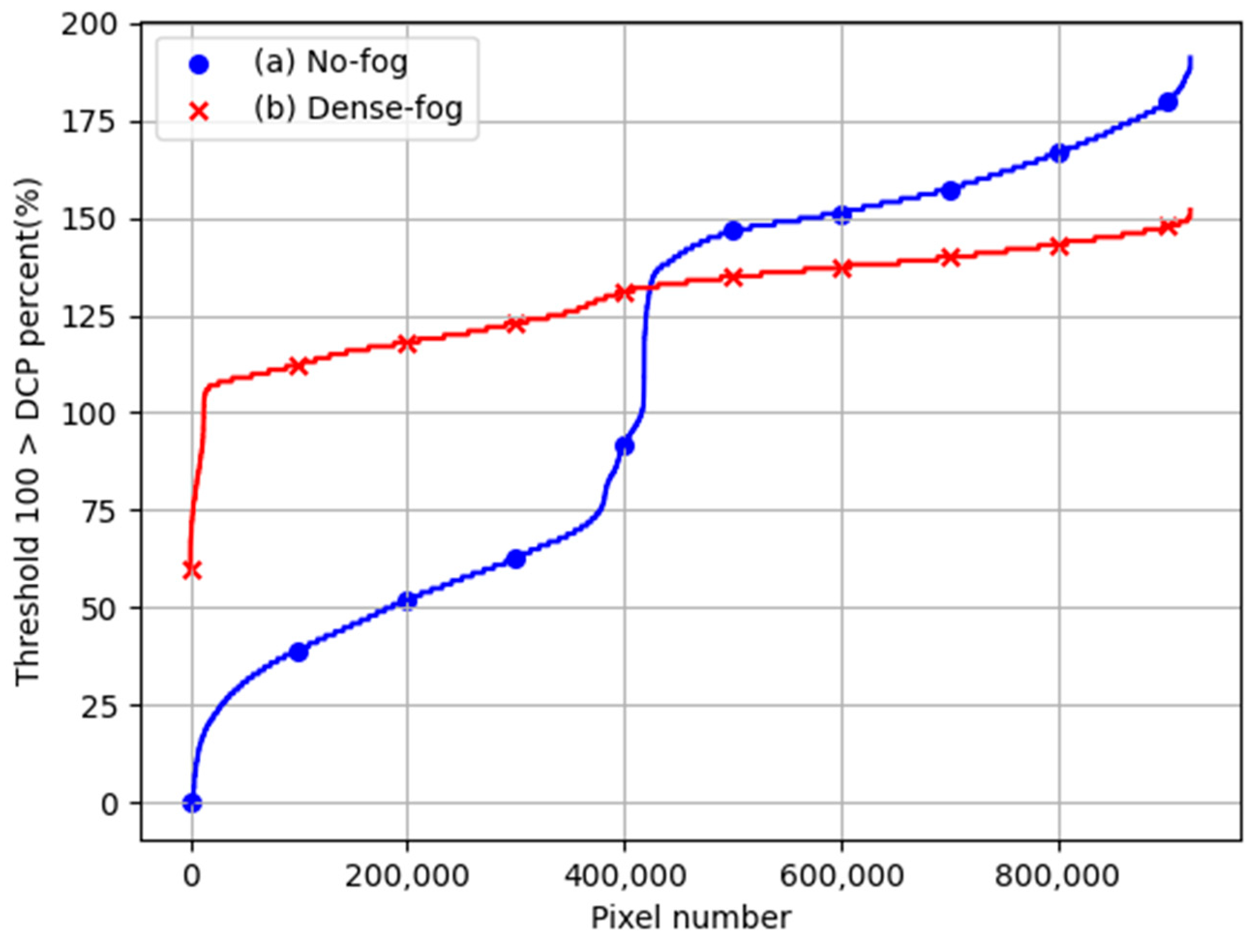
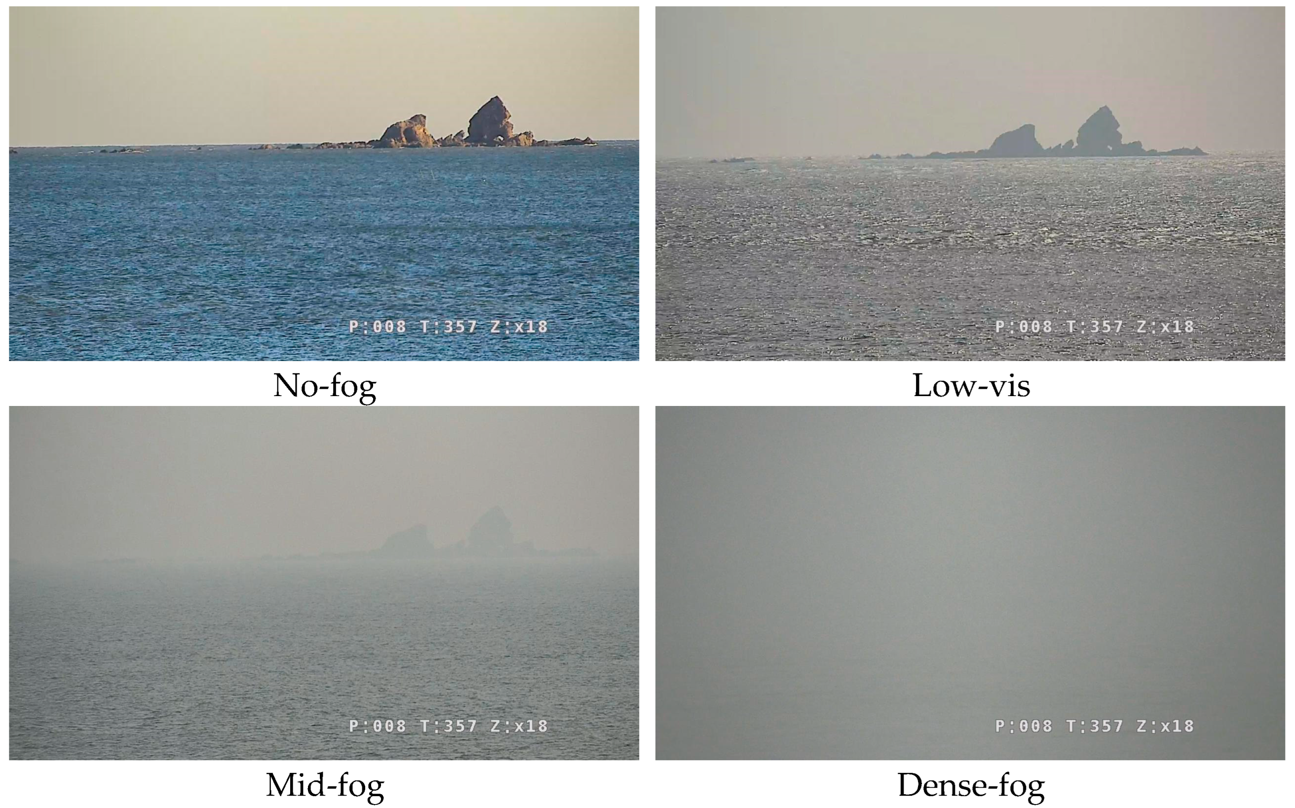
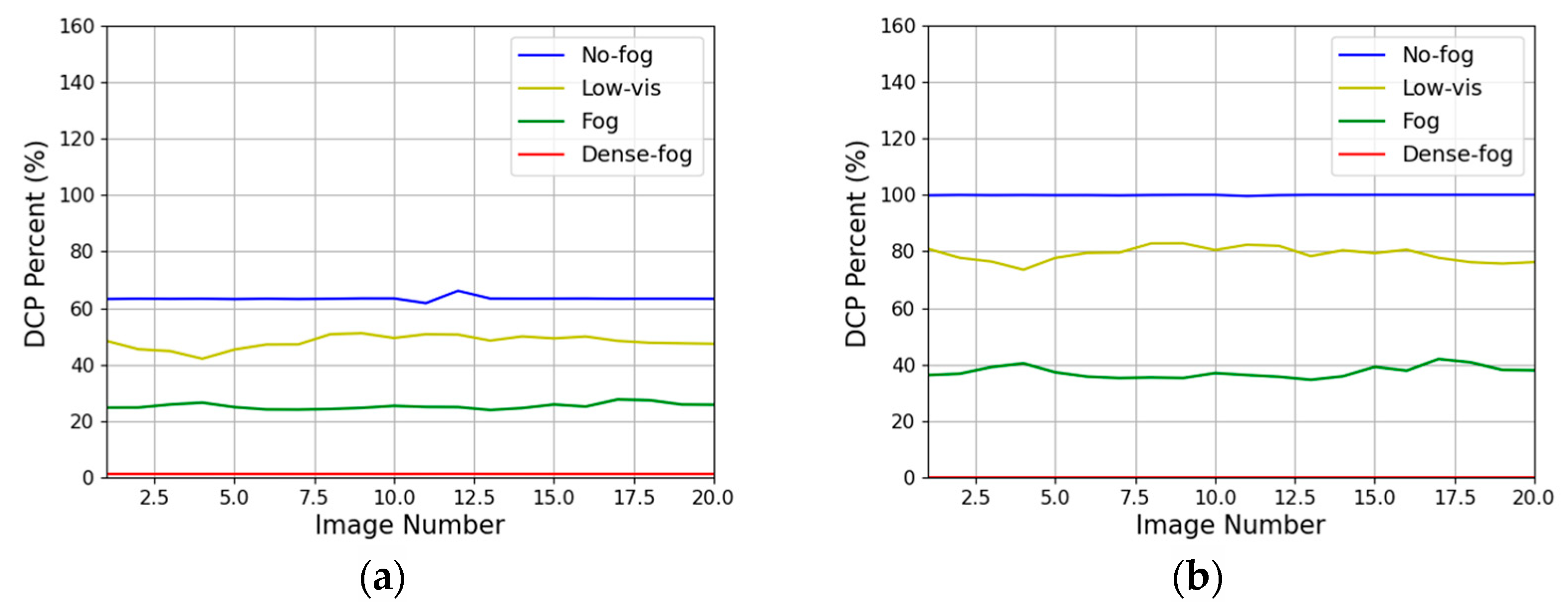
| Sea Fog Intensity | Visibility (Meters) | DC Percent (%) |
|---|---|---|
| No-fog | 1500~ | 75~100 |
| Low-fog | 1000~1500 | 50~75 |
| Mid-fog | 500~1000 | 25~50 |
| Dense-fog | 0~500 | 0~25 |
| Dataset | DCP Percent (%) |
|---|---|
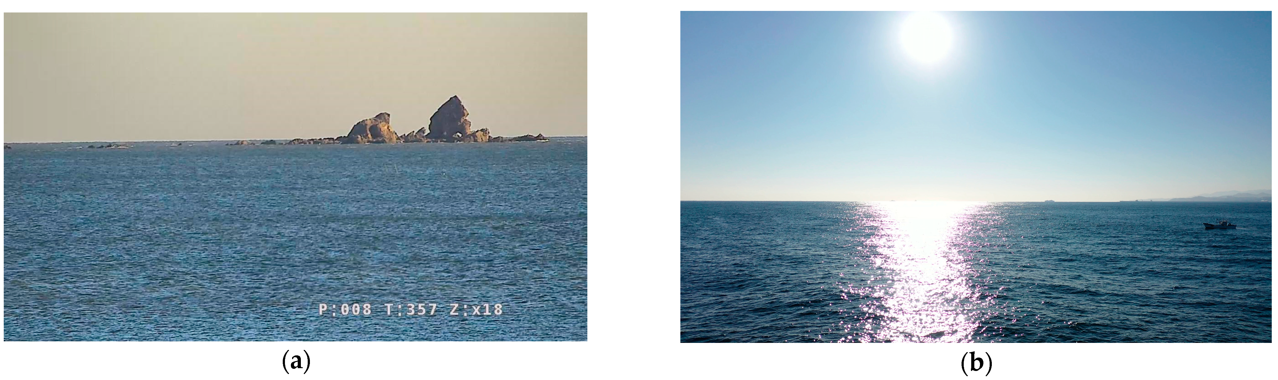
| Dataset (a) | 63% |
| Dataset (b) | 40% |
| Sea Fog Intensity | RDCP | AEA-RDCP |
|---|---|---|
| DCP percent | 85% | 100% |
| Processing time | 11 ms | 9 ms |
| Pixel count | 92,160 | 92,160 |
| State | No-fog | No-fog |
Disclaimer/Publisher’s Note: The statements, opinions and data contained in all publications are solely those of the individual author(s) and contributor(s) and not of MDPI and/or the editor(s). MDPI and/or the editor(s) disclaim responsibility for any injury to people or property resulting from any ideas, methods, instructions or products referred to in the content. |
© 2024 by the authors. Licensee MDPI, Basel, Switzerland. This article is an open access article distributed under the terms and conditions of the Creative Commons Attribution (CC BY) license (https://creativecommons.org/licenses/by/4.0/).
Share and Cite
Hwang, S.-H.; Kwon, K.-W.; Im, T.-H. AEA-RDCP: An Optimized Real-Time Algorithm for Sea Fog Intensity and Visibility Estimation. Appl. Sci. 2024, 14, 8033. https://doi.org/10.3390/app14178033
Hwang S-H, Kwon K-W, Im T-H. AEA-RDCP: An Optimized Real-Time Algorithm for Sea Fog Intensity and Visibility Estimation. Applied Sciences. 2024; 14(17):8033. https://doi.org/10.3390/app14178033
Chicago/Turabian StyleHwang, Shin-Hyuk, Ki-Won Kwon, and Tae-Ho Im. 2024. "AEA-RDCP: An Optimized Real-Time Algorithm for Sea Fog Intensity and Visibility Estimation" Applied Sciences 14, no. 17: 8033. https://doi.org/10.3390/app14178033
APA StyleHwang, S.-H., Kwon, K.-W., & Im, T.-H. (2024). AEA-RDCP: An Optimized Real-Time Algorithm for Sea Fog Intensity and Visibility Estimation. Applied Sciences, 14(17), 8033. https://doi.org/10.3390/app14178033