Abstract
Although Cyber–Physical Systems (CPSs) provide a flexible architecture for enterprises to deal with changing demand, an effective method to organize and allocate resources while considering sustainability factors is required to meet customers’ order requirements and mitigate negative impacts on the environment. The planning of processes to achieve sustainable CPSs becomes an important issue to meet demand timely in a dynamic environment. The problem with planning processes in sustainable CPSs is the determination of the configuration of workflows/resources to compose processes with desirable properties, taking into account time and energy consumption factors. The planning problem in sustainable CPSs can be formulated as an integer programming problem with constraints, and this poses a challenge due to computational complexity. Furthermore, the ever-shrinking life cycle of technologies leads to frequent changes in processes and makes the planning of processes a challenging task. To plan processes in a changing environment, an effective planning method must be developed to automate the planning task. To tackle computational complexity, evolutionary computation approaches such as bio-inspired computing and metaheuristics have been adopted extensively in solving complex optimization problems. This paper aims to propose a solution methodology and an effective evolutionary algorithm with a local search mechanism to support the planning of processes in sustainable CPSs based on an auction mechanism. To achieve this goal, we focus on developing a self-adaptive neighborhood search-based Differential Evolution method. An effective planning method should be robust in terms of performance with respect to algorithmic parameters. We assess the performance and robustness of this approach by performing experiments for several cases. By comparing the results of these experiments, it shows that the proposed method outperforms several other algorithms in the literature. To illustrate the robustness of the proposed self-adaptive algorithm, experiments with different settings of algorithmic parameters were conducted. The results show that the proposed self-adaptive algorithm is robust with respect to algorithmic parameters.
1. Introduction
Industry 4.0 has become a revolutionary industrial paradigm that can endow enterprises with the ability to fulfill challenging industrial and business requirements flexibly [1]. Cyber–Physical Systems (CPSs) offer a paradigm for realizing the vision of Industry 4.0 and support the daily operations of enterprises in the Industry 4.0 era [2]. Due to its capability to enable enterprises to monitor, manage and supervise resources and activities, the CPS becomes an important paradigm today. CPS refers to smart systems consisting of entities in cyber space and physical space. The entities in cyber space are computational components and the entities in physical space are physical components in the systems. CPS relies on interactions between the cyber-space computational components and physical-space components to achieve its goals through properly sensing, planning, control and monitoring. In the literature, a lot of studies concerning CPSs are available. Key research issues such as modeling [3,4,5], control [6], planning [7,8], security [9], development of context-aware applications [10] and resilience/robustness properties [11] have been studied in the context of CPSs. With the development of the Sustainable Development Goals (SDGs) aiming to achieve a more sustainable future [12], many countries around the world and companies in different sectors have been taking actions to achieve these SDGs. Therefore, the design of CPSs should take into account its sustainability factors. In the literature, sustainability in CPSs has been studied in [13,14,15]. Among the 17 SDGs, Goal 7, Goal 9, Goal 12, Goal 13 and Goal 17 are relevant to manufacturing. The challenges are the design and development of effective, energy-efficient and sustainable self-adaptive CPSs [16,17].
Recent studies on the energy efficiency and energy consumption of machine tools pave the way for the development of energy-efficient CPSs. Existing studies on the energy efficiency and energy consumption of machine tools can be found in the review papers [18,19]. The above studies provide the underpinning knowledge for developing effective, energy-efficient and sustainable self-adaptive CPSs. Although Cyber–Physical Systems (CPSs) provide a flexible architecture for enterprises to respond to changing demand and achieve the Sustainable Development Goals, an effective method to plan processes and allocate resources must be developed to realize these advantages in the Industry 4.0 era. An important related research subject in the context of CPSs is the sustainable development of the self-adaptive CPS [16]. Although a variety of approaches for the sustainable development of self-adaptive CPSs have been proposed in the literature [16], there lacks a sustainable development methodology that covers all the stages in the development of solvers for realizing self-adaptive CPSs, from modelling CPSs and problem formulation to the development of solution algorithms. The requirements of such a sustainable development methodology not only must be able to deal with a specific type of production process, achieving a specific goal of production using a specific solution algorithm, but also need to accommodate the changes in production processes, goals of production, and solution algorithms. To bridge this gap, this study focuses on developing a solution methodology to support the sustainable development of self-adaptive CPSs based on formal models, a general problem formulation and a solution algorithm for the general problem. We will illustrate the proposed framework by applying it to deal with the case of sequential production processes.
Self-organization and self-adaptation are two research issues related to exploiting the flexible architecture of a CPS to achieve production objectives [20,21,22] in the presence of unexpected changes or disturbances. The design of a CPS must consider issues in order to allow the system to self-organize and self-adapt to satisfy requirements dynamically [23]. To develop a self-organized and self-adaptive CPS, let us first review the architecture of a CPS. The design of a CPS can be divided into five levels [24], including the connection level, conversion level, cyber level, cognition level and configuration level. The collection of information from sensors, controllers or related systems in CPSs is conducted at the connection level. The transformation of the raw data into useful information is performed at the conversion level. The cyber level plays a central role in the architecture since it enables a CPS to interact with other CPSs and the environment. The cognition level constructs a virtual model based on the information gathered from all the components of the CPS. Knowledge of the CPS is generated at the cognition level to support decision-making. The configuration level deals with the self-configuration and self-optimization issues in the CPS. Planning and scheduling are two important issues in the Industry 4.0 literature [25,26] and are at the configuration level in CPS design [27]. The scheduling issue has been studied in [3,10,11] under the premise of pre-specified workflows of processes and capabilities of resources in CPSs. However, the workflows of processes and capabilities/efficiency of resources may change dynamically. In addition, the energy consumption factor is not considered in [3,10,11]. Developing a method to determine the configuration of workflows and resources is urgent. Process planning aims to determine the configuration of the production process and the associated resources involved. It is a preliminary step for developing a self-organized and self-adaptive CPS and solving the subsequent scheduling problem [28]. The planning of CPSs with logistic models has been studied in [29]. The process planning issue in CPS design has been studied in [30]. However, the sustainability factor of CPSs is not considered in [30].
This paper focuses on the problem of determining the configuration of workflows/resources to compose processes with desirable properties in planning sustainable CPSs. Time and energy consumption are two important factors in developing production processes for sustainable CPSs. The former focuses on the issue of meeting the order demand in a timely manner, whereas the latter is directly related to the sustainability issue in the manufacturing sector. Therefore, time and energy consumption factors must be taken into consideration in the production planning processes in sustainable CPSs. In addition to time and energy consumption factors, planning production processes in CPSs must be based on the operational requirements/constraints of the processes and the real-time information available from the IoT infrastructure.
The planning of processes in sustainable CPSs is an important issue to timely meet demand and sustainability development goals. The ever-shrinking life cycle of technologies leads to frequent changes in processes. This makes the planning of processes a challenging task. To plan processes in the presence of process changes, an effective planning method must be developed to automate the planning task. A CPS consists of entities in cyber space and physical space. Cyber World models are used to capture the capability of entities in the CPS. To address the planning problem, proper modeling tools must be used to construct the Cyber World models for the CPS. Petri nets are applied to model and manufacturing systems [31] due to their capability to capture discrete events, as well as synchronous/asynchronous and concurrent operations in production systems. In particular, Discrete Timed Petri Nets (DTPNs) have been applied to represent the Cyber World models for the CPS, solve the scheduling problems [3,10] and assess the influence of failures on the CPS [11]. In this study, DTPNs are adopted as the Cyber World models for the CPS. However, the problem addressed in this study is to determine the DTPNs necessary to meet the manufacturing requirements of sustainable CPSs instead of analyzing given DTPNs.
In the literature, the planning of processes in CPSs were studied. For example, in [27,28,29,30], different approaches were proposed for planning processes in CPS. This study aims to develop a more effective evolutionary algorithm for planning processes in CPS based on an auction mechanism. Auctions have been applied in transportation service procurement on the Cyber–Physical Internet [32] in on-demand logistics trading [33], cloud manufacturing resource trading [34] and task allocation in CPSs [35]. In this study, an auction mechanism will be used in the CPS over the course of the process planning. As the process-planning problem is a constrained discrete optimization problem, an effective approach must be used to tackle its complexity issue. Due to the success of applying various evolutionary computation approaches in the literature to optimize CPSs [36,37,38], we will adopt an evolutionary computation approach to solve the planning problem of sustainable CPSs.
Well-known evolutionary computation approaches include Particle Swarm Optimization [39] and Differential Evolution [40,41,42]. In the literature, the effectiveness of an evolutionary computation algorithm can be assessed based on performance and robustness. Performance is concerned with the quality of solutions found and is usually measured with the average fitness function values of solutions. In addition to performance, robustness is also an important metric in the evaluation of metaheuristic algorithms [43,44]. The robustness of an evolutionary computation algorithm is measured by the sensitivity of the average fitness function values with respect to the algorithmic parameters. In this study, we will develop an effective evolutionary algorithm for planning production processes in sustainable CPSs and study the computational experiences of the solution algorithm in terms of performance and robustness.
In the literature, the neighborhood search mechanism is an effective approach to solving optimization problems. Self-adaptive mechanisms provide an approach to adapting the parameters of a solution method. Combining these two mechanisms has the potential to yield a better solution in the solution space [45]. The effectiveness of this approach has been successfully applied in [46]. To achieve the goal of this study, we focus on developing a self-adaptive neighborhood search-based Differential Evolution method to support the planning of processes in sustainable CPSs. In this study, a self-adaptive mechanism is combined with neighborhood search in the Differential Evolution method. This creates a self-adaptive neighborhood search Differential Evolution (SaNSDE) algorithm. To tackle the constraints of the planning problem, the method used in [47] is adopted. We assess the performance of this approach by performing experiments for several cases. By analyzing the results of these experiments, it shows that the proposed method outperforms several methods in the literature.
This paper differs from the previous ones on CPSs in [3,11] in that both the sustainability factor and efficiency factor are jointly considered in this study. The contributions of this paper are as follows. First, a general problem formulation for planning processes considering time and sustainability factors is proposed. Second, a solution method for the problem based on the self-adaptive mechanism and neighborhood search mechanism is proposed. Third, the proposed method is verified by a special class of production processes. Fourth, the effectiveness of the proposed solution algorithm in terms of performance and robustness is studied and shows that the proposed solution algorithm outperforms several other algorithms.
We structure the rest of this paper as follows. In Section 2, we first describe the problem in planning processes in a CPS by briefly introducing the optimization problem. In Section 3, we will propose a SaNSDE algorithm based on the DE approach. We will report the experimental results in Section 4. We will discuss the results in Section 5 and conclude this paper in Section 6.
2. Modeling and Problem Formulation
We will first start with a motivating example, introduce the models of entities in CPS and then formulate the problem in planning a process in a sustainable CPS. We consider several factors in the process-planning problem, including operational requirements, time for executing operations, energy consumption of operations and constraints of the processes.
A Motivating Example: Consider a CPS consisting of a number of process agents, resource agents and optimization agents. The role of a process agent is to specify the requirements of the target production process to be planned and submit the requirements to the optimization agent. The role of a resource agent is to specify the operations that it can perform and submit bids to the optimization agent to indicate the potential operations that can be performed by it. The optimization agent aims to determine the optimal configuration of the process agent and resource agents based on the bids submitted by the process agent and the resource agents. For example, suppose the workflow of process agent requires five operations to be performed. Suppose the upper bound of the processing time of the process to be composed for process agent is = 200. Suppose there are nine resource agents in the CPS to perform operations. Depending on the type of resource agents, the capability varies. That is, the function of different types of resource agents is different in general. Therefore, each type of resource agent can only perform some of the operations. The planning problem for process agent is to find the configuration of resource agents that can completely perform the required operations, satisfy the processing time requirement and optimize energy consumption. To address this process-planning problem in the CPS, several Cyber World models must be defined to capture the operations, the workflow of the process agent and the capability of resource agents (activities that can be performed by resource agents).
The above motivating example used to illustrate the proposed solution method is based on a real application scenario similar to the one reported in [48]. The difference between the illustrative example used in this paper and the one in [48] is the number of resource agents and the number of operations in the process. Please refer to [48] for the details of the application scenario.
2.1. A Multi-Agent System Architecture and Models of Agents in CPSs
In this subsection, we introduce the models of CPSs. A process in a CPS consists of a number of operations. The execution of operations must satisfy their constraints as needed. The operations may be performed by different resources. A multi-agent system architecture is used in this study to model the process-planning problem in CPSs. The entities involved in the process planning of a CPS include process agents, resource agents and optimization agents. Agents interact with each other in the CPS with a multi-level contract net protocol (CNP) [10].
Each process agent specifies the requirements of a production process. A process agent submits a bid to describe the requirements of its production process. Each resource agent in the CPS represents a manufacturing resource that performs operations in the production process. A resource agent submits bids according to its capabilities to perform different operations. An optimization agent aims to determine the configuration of a process agent and relevant resource agents to realize the production process according to the bids of the process agent and resource agents.
Using different combinations of resources to perform the required operations typically results in different total processing time and energy consumption for the process. The total processing time and energy consumption of a process are two important characteristics that need to be optimized. To obtain a process with satisfactory characteristics in a CPS, an objective function is required. An objective function that considers both total processing time and energy consumption is defined. Given the objective function, a constrained optimization problem is formulated for the process-planning problem. The problem of planning processes in CPSs is to find the winning bids (the best combination of bids) based on the bids submitted by resources such that the objective function is optimized.
To describe the capabilities of agents and formulate the planning problem, a list of notations is defined in Table 1.

Table 1.
Notations used in the models and problem formulation.
The requirements of a process agent in the CPS are specified by the operations and the connection between operations. We construct the Cyber World model for the -th operation of process agent and the Cyber World model for process agent as follows.
In this paper, we adopt Discrete Timed Petri Nets (DTPNs) to represent the Cyber World model of an activity.
A DTPN is described by , where denotes a set of places, denotes a set of transitions, denotes a set of flow relations, denotes the initial marking, the function specifies the firing time for each transition and is the set of nonnegative integers.
Definition 1.
The Cyber World model for the -th operation of process agent is a DTPN with = and = , where denotes the start transition, denotes the end transition, denotes the busy state place of the -th operation and denotes a function specifying the firing time of each transition in .
For the motivating example, to represent the operations, a model is constructed for each operation. As there are five operations for the workflow of process agent , we will construct models, , , , and , to represent these five operations.
Figure 1a–e show the DTPN models , , , and for the first operation, the second operation, the third operation, the fourth operation and the fifth operation, respectively.

Figure 1.
The Cyber World models for the five operations of process agent : (a) the DTPN model for the first operation; (b) the DTPN model for the second operation; (c) the DTPN model for the third operation; (d) the DTPN model for the fourth operation; (e) the DTPN model for the fifth operation.
For the example in Figure 1, the start transition of is and the end transition of is . The start transition of is and the end transition of is . Similarly, , , , , and . The busy state place of is , the busy state place of is , the busy state place of is , the busy state place of is and the busy state place of is .
To construct the Cyber World model for process agent , we combine the Cyber World models of the operations involved. A operator is defined to combine two DTPNs.
Definition 2.
Given two DTPNs, = (, , , , ) and = (, , , , ), = (, , , , ), where , , , and .
Let denote the maximum number of operations involved in the workflow of process agent . We define the Cyber World model of process agent as follows.
Definition 3.
The Cyber World model of process agent , where is an acyclic DTPN = .
Figure 2 shows the DTPN model, , for process agent , where

Figure 2.
The DTPN model of a process agent, where = .
Operations in a CPS are performed by the resource agents. In this paper, the action that an agent performs an operation is called an activity. An activity can be described by a Cyber World model.
Let denote the Cyber World model described by a DTPN of the activity performed by resource agent for -th operation of process agent , defined as follows.
Definition 4.
We use DTPN as the Cyber World model to represent that the -th operation of
process agent is
performed by
resource
agent
, where , the initial marking is the number of available resources and is the idle state place. There is no common transition between and for .
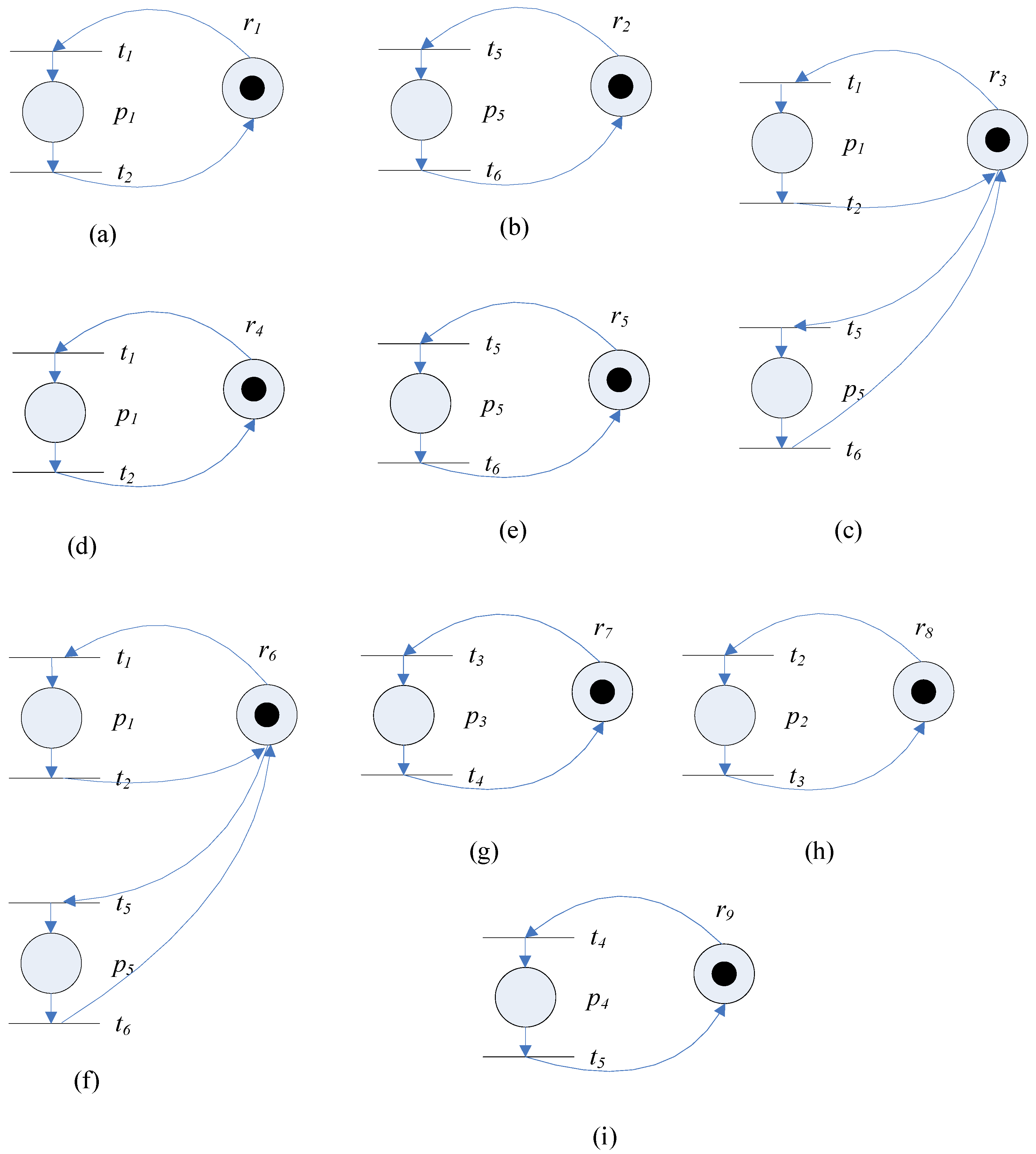
For the motivating example, to represent the capability of a certain type of resource agents, we will construct the resource activity model for each type of resource agent. We use the resource activity model to denote the activity that the -th operation of process agent can be performed by resource agent . In this example, the resource activity model for resource agent is , the resource activity model for resource agent is , the resource activity model for resource agent is , the resource activity model for resource agent is , the resource activity model for resource agent is , the resource activity model for resource agent is , the resource activity model for resource agent is , the resource activity model for resource agent is and the resource activity model for resource agent is .
Figure 3 shows the resource activity models for the resource agents in the motivating example.
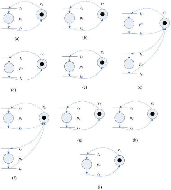
Figure 3.
Examples of resource activity models for resource agents. (a) ; (b) ; (c) ; (d) ; (e) ; (f) ; (g) ; (h) ; (i) .
The set of resource agents for performing the -th operation in is denoted by . The set of resource agents for performing the operations in is denoted by .
A configuration for process agent is defined by the Cyber World model, , of process agent and the Cyber World models of activities of resources agent for performing the operations in .
Definition 5.
The Cyber World model for a configuration of process agent with the Cyber World model and the Cyber World models of activities of resources agent for performing the operations in is a DTPN = = , where . The firing time for each transition is .
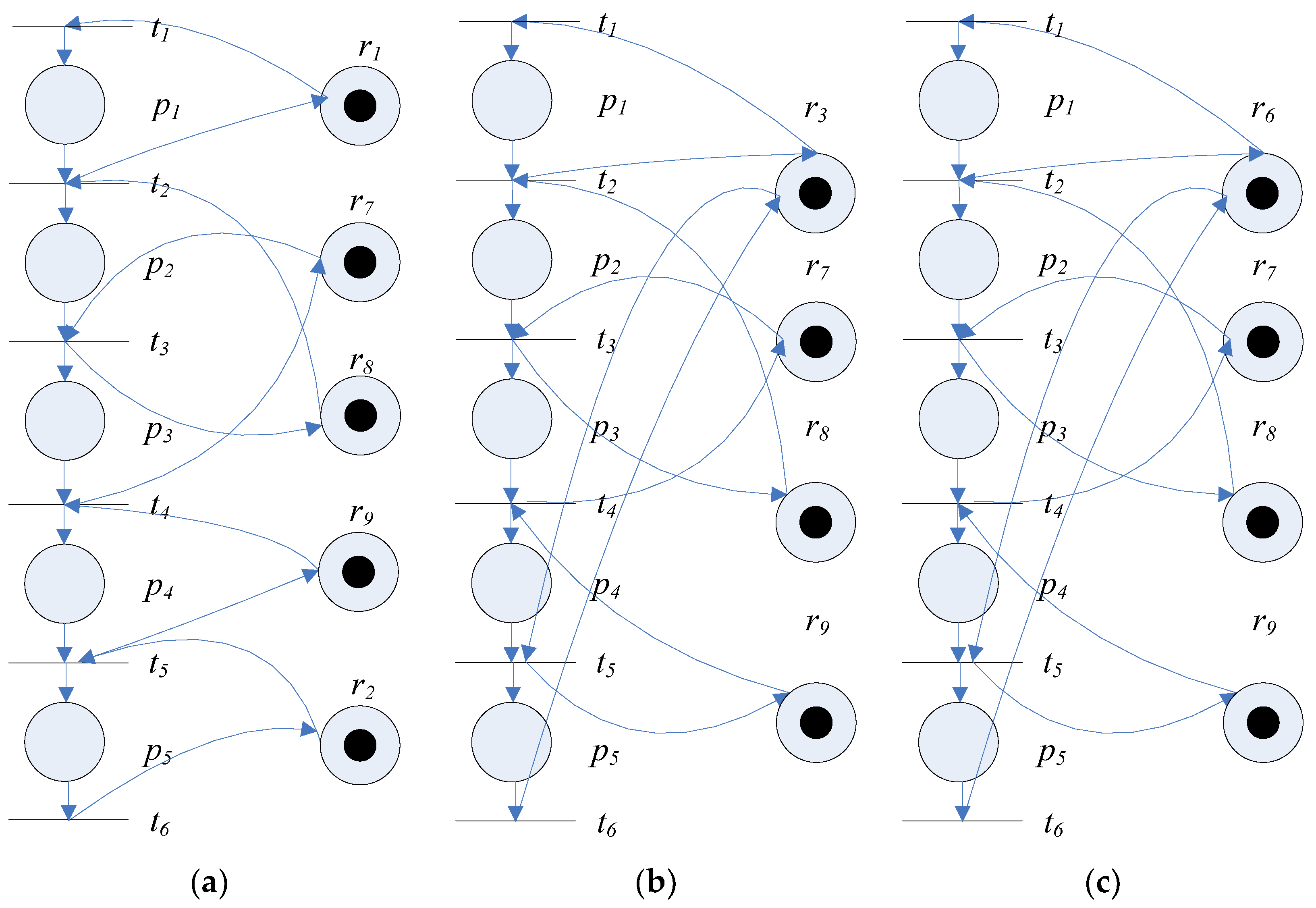
Note that the number of different configurations of process agent is usually not unique. For example, Figure 4a–c show three different configurations for process agent . The process-planning problem is to find the optimal configuration of the process agent and the associated set of resource agents for performing the -th operation in to compose the overall Cyber World model = = to meet the manufacturing requirements.
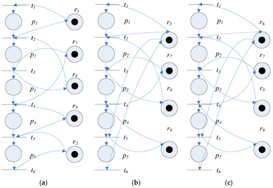
Figure 4.
(a) The Cyber World model for the configuration ; (b) the Cyber World model for the configuration ; (c) the Cyber World model for the configuration .
2.2. Process-Planning Problem Formulation for Sustainable CPS
In this subsection, the process-planning problem will be formulated for a sustainable CPS. We use to represent the requirements of the process agent . can be specified based on the operations in the production process and the desirable properties of the production process. For example, suppose the process agent requires a number of operations to be performed and the upper bound of total processing time is . Let be the maximum number of operations in the workflow of process agent . In this case, can be described by , where is equal to 1 if operation is required to be performed in the requirements of process agent , is equal to 0 otherwise and the overall processing time must be no greater than .
In this study, we use the concept of agents to model resources in CPS. A CPS consists of a set of resource agents such as machine agents and robot agents. The set of agents in the system is denoted by . Each agent is autonomous and may submit bids in the CPS to indicate its capability to perform a set of operations. A bid indicates the capability for the resource agent to perform operations in the requirements of the process agent .
We use to represent the number of bids submitted by resource agent . The j-th bid submitted by a resource agent is denoted by = , where is one if operation can be performed by resource agent in the j-th bid, is zero otherwise and is the overall processing time for performing the specified operations. The set of all bids is denoted by = {, where and }.
Based on the resource activity model, each resource agent submits bids to indicate the operations it can perform. For the motivating example, the resource activity model for resource agent consists of transition and transition . As transition is the start transition of Cyber World model and transition is the end transition of Cyber World model , resource agent can perform the first operation. Therefore, resource agent submits a bid = = , where 25 is the processing time of resource agent for the first operation. Other types of resource agents also submit bids similarly.
The energy consumption information of the j-th bid submitted by agent is denoted by = , where is the overall energy consumption for performing the specified operations in the bid. The set of energy consumption information for all bids is denoted by = {, where and }.
We use to denote the decision variable of the optimization problem. The value of is one if the j-th bid of agent is accepted and is zero otherwise.
To assess the quality of a process in CPS, an objective function that considers both total processing time and energy consumption is defined. We use to denote a function that calculates the total processing time of a configuration of process agent based on the solution and , where and . We use to denote a function that calculates the energy consumption according to the solution and , where and .
To propose a general framework to support the planning of processes in sustainable CPSs, a general form of the objective function is first presented. The general form of the objective function will be tailored for the case of sequential processes to illustrate its usage next. The general form of the objective function is a function of the decision variable, . Therefore, we use to denote the objective function. As the cost due to the total processing time and energy consumption factors are considered in this study, the objective function is a function of the total processing time of the configuration calculated by and the energy consumption of the configuration calculated by . Therefore, is described by . Note that is related to time, whereas is related to energy consumption. There are several different ways to combine and to define the objective function . For example, one may introduce weighting coefficients to combine and to define the objective function . Alternatively, one may define as the weighted sum of functions of and , e.g., = , where is a monotonic decreasing function and is a monotonic increasing function.
The objective function should be tailored properly according to the characteristics of the type of production processes under consideration and the goal of the production process. We will elaborate for the special case of sequential processes later to illustrate how the objective function is defined.
In our problem formulation, we use to denote the constraints to satisfy the requirements of the operations specified in . We use to denote the constraints to satisfy time requirements specified in . We use to denote the other types of constraints. We formulate the following problem to maximize the objective function.
s.t.
The problem formulation defined by (1) through (5) should be tailored properly according to the characteristics of the type of production processes under consideration and the goal of the production process.
To illustrate how to tailor the problem formulation defined by (1) through (5) to create a process with desirable properties, let us consider the problem of composing a process for a process agent with a sequential Cyber World model in a CPS. Suppose the composed process must satisfy three requirements: (i) each operation in the process must be performed by an agent, (ii) the total processing time of the process must be no greater than a given upper bound and (iii) the number of times an operation can be performed by each agent cannot exceed a pre-specified upper bound .
In this case, we may tailor the problem defined by (1) through (5) for composing a sequential process as follows. If the is a sequential process, the constraints to satisfy the requirements of the operations can be represented by . If is a sequential process, . Let denote the upper bound of the total processing time of the process . In this case, the constraints to satisfy the time requirements can be represented by . Suppose we want to set an upper bound on the maximum number of times that an operation can be performed by each agent. The constraints can be represented by .
We define as an increasing function of and a decreasing function of . For example, . We formulate the following problem to maximize the objective function.
The problem defined in (6) through (10) aims to find a solution that maximizes the objective function , where and , such that the requirement of the process is satisfied, the total processing time of the overall process cannot exceed and the maximum number of times that an operation can be performed by each agent cannot exceed .
3. The Algorithm
In this section, the SaNSDE algorithm will be proposed. As the SaNSDE algorithm is a variant of the Differential Evolution algorithm, it is a class of evolutionary algorithm that relies on a properly defined fitness function to assess the quality of a potential solution. We present the fitness function used in this paper first and the SaNSDE algorithm next.
3.1. Fitness Function
Just like other evolutionary algorithms, the SaNSDE algorithm relies on a properly defined fitness function that considers both the objective function values and constraint violations. We define a fitness function based on the method proposed in [47]. We use to denote the set of all feasible solutions in the current population. For the problem defined by (1) through (5), we define fitness function as follows:
is the penalty of constraint violation of ,
is the penalty of constraint violation of and
is the penalty of constraint violation of .
For the process-planning problem of a sequential process defined by (6) through (10), the fitness function is defined as follows:
3.2. SaNSDE Algorithm
To describe the self-adaptive algorithm, the notations are defined in Table 2.

Table 2.
Notations of symbols, variables and parameters used in the proposed algorithm.
As the decision variables are represented by the vector , the solution is represented by a vector. Therefore, each individual in the population is also a vector. We use to denote the -th individual in the population. The dimension of is the same as that of . We use to denote the dimension of . The element in the -th dimension of is denoted by . We use to denote the mutant vector of the -th individual in the population. The dimension of is the same as that of . The element in the -th dimension of is denoted by . We use a to denote the trial vector of the -th individual in the population. The dimension of is the same as that of . The element in the -th dimension of is denoted by . We use to denote the binary transformation function to transform a trial vector to a binary vector. This binary transformation function is the same as the one used in [46].
The SaNSDE algorithm basically follows the three steps of the standard Differential Evolution approach: mutation, crossover step and selection. The scale factor is generated randomly. The generation of the scale factor depends on whether a randomly generated value from is less than . If is less than , the scale factor will be generated from the Gaussian distribution . Otherwise, the scale factor will be generated from the uniform distribution . A random value will be generated from to determine which mutation strategy will be used. If , mutation strategy = 1 and the mutant vector will be calculated by . Otherwise, mutation strategy = 2 and the mutant vector will be calculated by . Following the mutation operation, a trial vector will be calculated and the individual will be updated as needed. The successful or failed update counter will be updated as needed. The value of will be updated according to the successful or failed update counter after the learning period .
Based on the notations above, the proposed self-adaptive neighborhood search Differential Evolution algorithm is defined in Algorithm 1 as follows.
| Algorithm 1: SaNSDE Algorithm |
| Step 0: Initialize parameters = 0.5 and = 0.5 |
| Generation of random population with individuals |
| Set the learning period |
| = 0.5 |
| Initialize a population with individuals randomly |
| Step 1: For |
| For |
| Step 1.1: Generate with uniform distribution |
| If |
| Generate with Gaussian distribution |
| Else |
| Generate with uniform distribution |
| End If |
| Generate with Gaussian distribution |
| Step 1.2: Generate |
| For {1, 2, …, } |
| If |
| Else |
| End If |
| End For |
| Step 1.3: Trial vector computation |
| For {1, 2, …, } |
| End For |
| Step 1.4: |
| Individual update |
| If |
| = |
| Record in |
| Else |
| End If |
| End For |
| If |
| End If |
| End For |
4. Results
We conducted several experiments to assess the performance and efficiency of the SaNSDE algorithm. We will first present the results of a small example in Section 4.1. In Section 4.2, we will compare the performance/efficiency of the proposed algorithm with other ones. In Section 4.3, we will present the results on the influence of the learning period parameter on the performance/efficiency of the proposed algorithm. The statistical significance of the results will be presented in Section 4.5.
4.1. A Small Example
We applied the SaNSDE algorithm proposed in Section 3.2 to find the solutions for several cases. Comparison with other algorithms based on results of experiments will be presented in the next subsection. We first illustrate the proposed method by applying it to the motivating example in Section 2.
In this example, we consider a planning problem for a process agent with five operations to be performed by resource agents. Suppose the upper bound of the processing time of the process is = 200. The DTPN models, , , , and for the first operation, the second operation, the third operation, the fourth operation and the fifth operation, respectively, are shown in Figure 1a–e. As there are five operations to be performed, the requirements of the process agent are described by . In this case, , and . The model of the process agent is shown in Figure 2.
Suppose there are nine types of resource agents in the CPS to perform the five operations. Each type of resource agent can only perform a subset of the five operations. The capability of each type of resource agents is described by the resource activity models in Figure 3. Based on the resource activity model, each resource agent submits a bid to indicate the operations it can perform. For example, the resource activity model for resource agent consists of transition and transition . As transition is the start transition of Cyber World model and transition is the end transition of Cyber World model , resource agent can perform the first operation. Therefore, resource agent submits a bid = = , where 25 is the processing time of resource agent for the first operation. Similarly, the resource activity model for resource agent consists of transition and transition . As transition is the start transition of Cyber World model and transition is the end transition of Cyber World model , resource agent can perform the fifth operation. Therefore, resource agent submits a bid = = , where 25 is the processing time of resource agent for the fifth operation. The resource activity model for resource agent consists of transitions , , and . As transition is the start transition of Cyber World model and transition is the end transition of Cyber World model , resource agent can perform the first operation. As transition is the start transition of Cyber World model and transition is the end transition of Cyber World model , resource agent can perform the fifth operation. Therefore, resource agent submits a bid = = , where 45 is the processing time of resource agent for the first operation and the second operation. Based on the corresponding resource activity models, resource agents through also submit their bids. The information on all the bids submitted by resource agents is shown in Table 3 and Table 4.

Table 3.
The information of processing time of bids in .

Table 4.
The information of energy consumption of bids in .
The algorithmic parameters used by the SaNSDE algorithm and NSDE algorithm are listed as follows:
The parameters of the SaNSDE algorithm are as follows.
The number of iterations: 10,000
Population size (): 30
The objective function used is , where = 1 and = 1. The following solution is found by the proposed algorithm: . The configuration of our solution is the bids submitted by the set of resource agents {3, 7, 8, 9}. This solution corresponds to the Cyber World model for the configuration in Figure 4b. The processing time achieved for this solution is 45 + 40 + 28 + 32 = 145. The fitness function value found for this example is 42.
For this example, there are several candidate configurations that can perform all the operations in the process. These candidate configurations include the bids submitted by the sets of resource agents { 1, 2, 7, 8, 9 }, { 1, 5, 7, 8, 9}, {3, 7, 8, 9}, {4, 2, 7, 8, 9}, {4, 5, 7, 8, 9} and {6, 7, 8, 9}. The values of the fitness function defined in Section 3.2 for these candidate configurations are 42, 32, 42, 32, 22 and 27, respectively. The configuration of the solution found by the proposed algorithm is the bids submitted by the set of resource agents {3, 7, 8, 9}, which is optimal as the value of the objective function is maximal. So, the solution found is consistent with our expectation.
4.2. Comparison with Other Algorithms
To illustrate the effectiveness of the SaNSDE algorithm proposed in Section 3.2, the PSO algorithm, six standard DE algorithms (DE1 through DE6) and a variant of the neighborhood search-based DE (NSDE) algorithm [49] were used for comparison with the proposed algorithm. There are two reasons to compare it with these algorithms. First, these algorithms had been applied to the special case of the problem considered in this paper, in which the energy consumption factor is not considered in the objective function (i.e., = 0 in (6)) but the constraints are the same. Second, these algorithms had also been successfully applied to solve complex constrained optimization problems with binary decision variables such as the ones in the studies [50,51]. Therefore, we compared the proposed algorithm with these eight algorithms. We performed experiments by applying these algorithms to solve ten instances. We recorded and analyzed the results to compare the performance and efficiency of the different algorithms.
All the algorithms mentioned above are population-based algorithms. Population size () is a parameter for all these algorithms. As the performance of different evolutionary algorithms may depend on population size, we consider a small population size of 10, a moderate population size of 30 and a larger population size of 50 to conduct the experiments in this study. The small population size is used to test whether all these algorithms can work effectively even if the total number of individuals in the population is small. By comparing the results obtained with a small population size of 10, a moderate population size of 30 and a larger population size of 50, we will be able to know which algorithms are sensitive to the population size parameter. In this subsection, we first present the results of experiments for the population size = 10. The results of experiments for the population sizes = 30 and 50 will be presented next.
In addition to the population size parameter, the other parameters used in the different algorithms are as follows.
The parameters used in the discrete NSDE algorithm are as follows.
= , where is a random value with a Gaussian distribution .
The number of iterations: 10,000
The parameters used in the discrete Particle Swarm Optimization algorithm are as follows.
The number of iterations: 10,000
The parameters used in the discrete Differential Evolution algorithm are as follows.
: a value arbitrarily selected from uniform (0, 2)
The number of iterations: 10,000
Table 5 and Table 6 show the results for the population size = 10, obtained by applying the SaNSDE algorithm, a variant of the neighborhood search-based DE (NSDE) algorithm, the PSO algorithm and six standard DE algorithms.

Table 5.
Fitness function values for discrete SaNSDE, NSDE and PSO with population size = 10.

Table 6.
Average fitness function values for DE1, DE2, DE3, DE4, DE5 and DE6 with = 10.
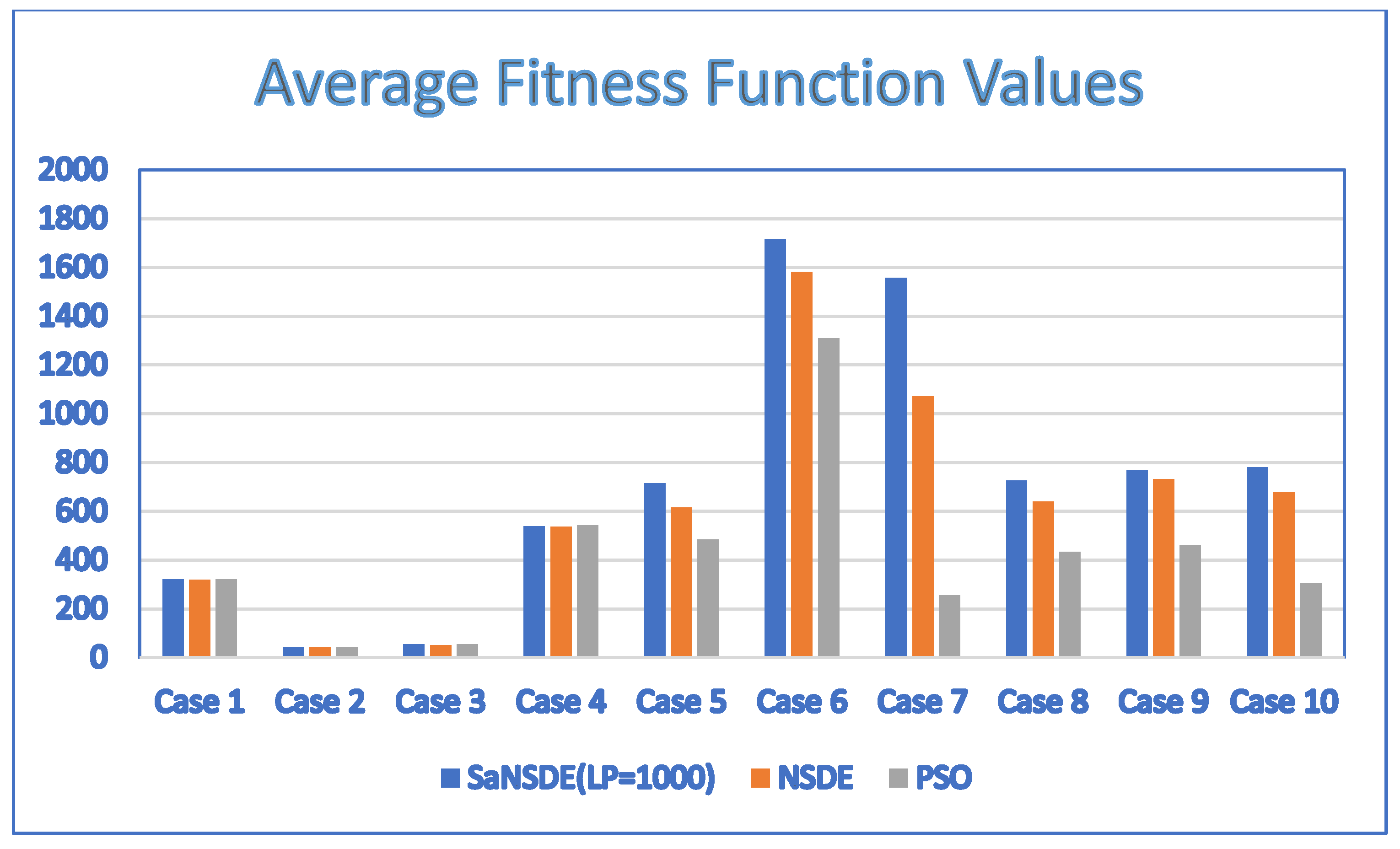
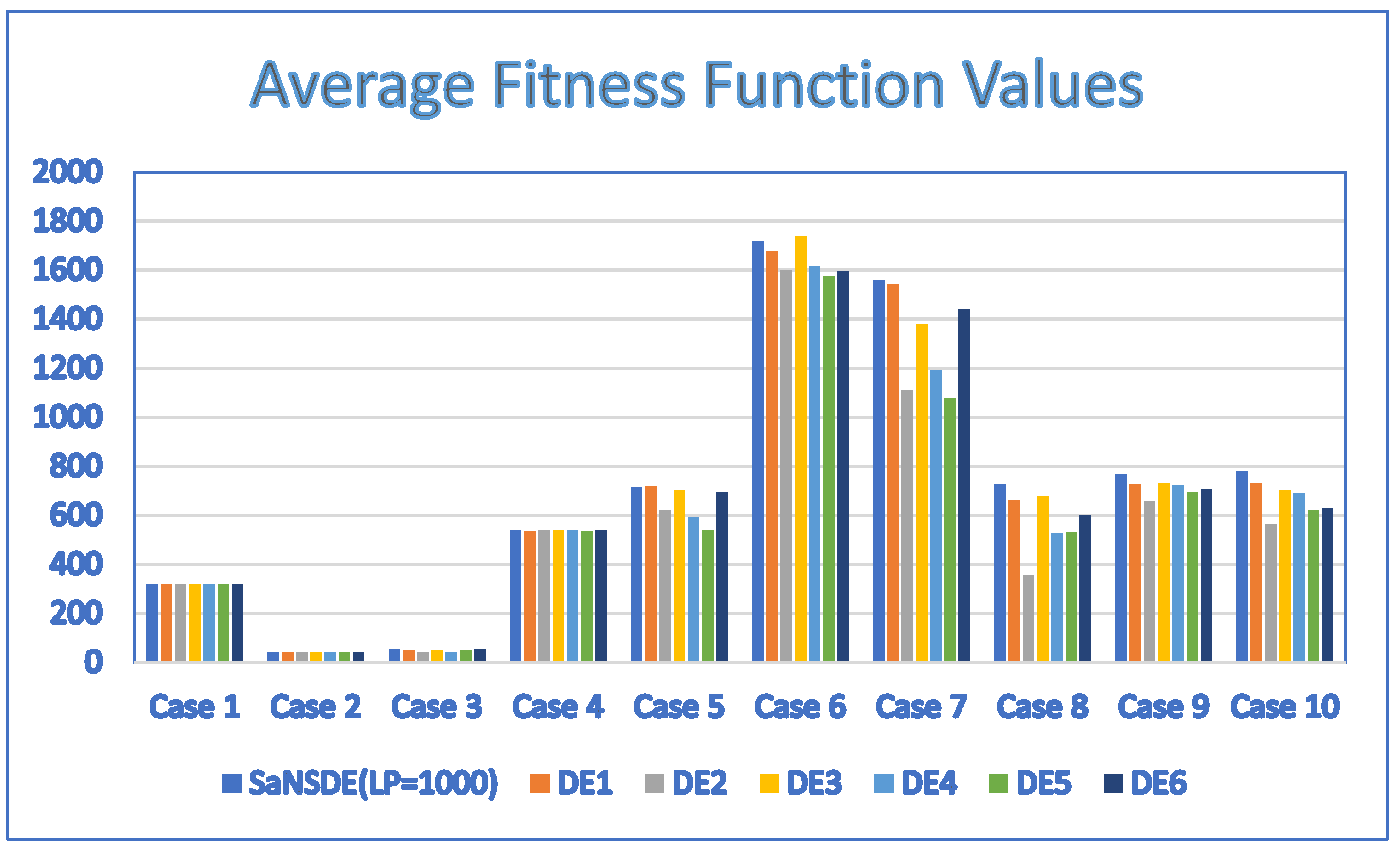
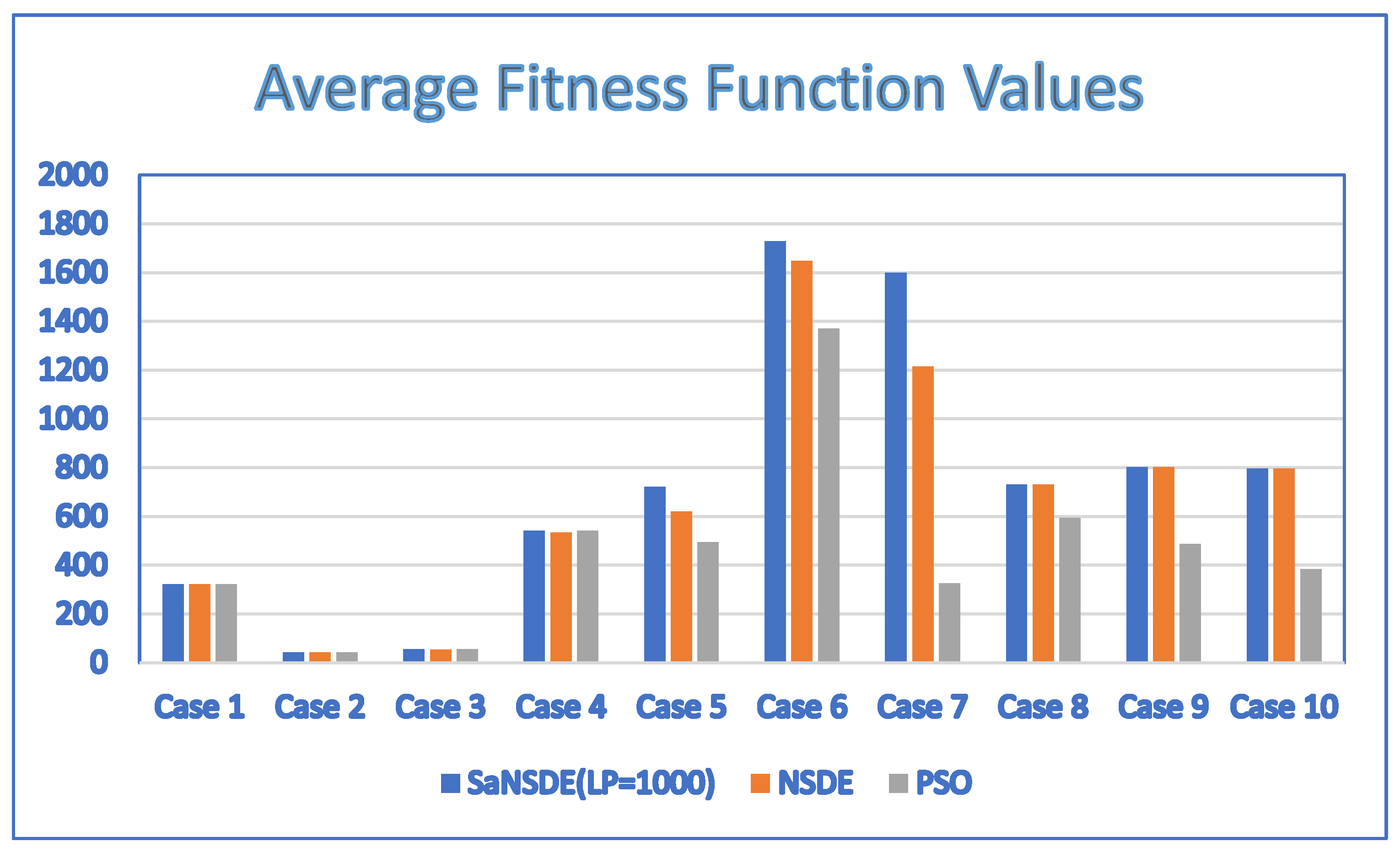
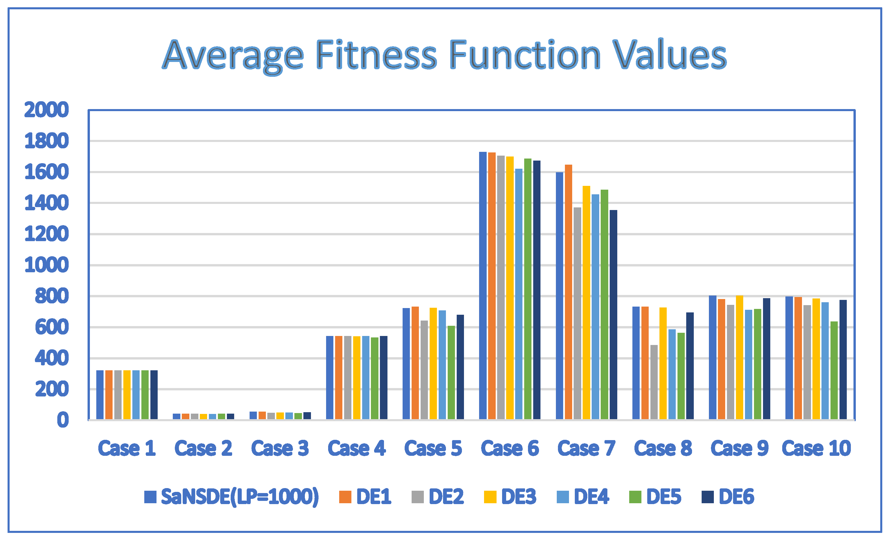
In terms of performance, the results of Table 5 indicate that the SaNSDE algorithm either outperforms or performs as well as the NSDE algorithm and PSO algorithm for most instances, with the exception of Case 4. The average fitness function values in Table 5 and Table 6 are shown in the bar charts of Figure 5 and Figure 6, respectively.
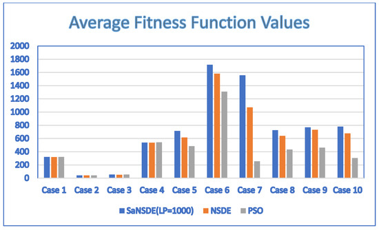
Figure 5.
Average fitness function values for discrete SaNSDE (LP = 1000), NSDE and PSO with = 10.
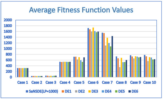
Figure 6.
Average fitness function values for discrete SaNSDE (LP = 1000), DE1, DE2, DE3, DE4, DE5 and DE6 with = 10.
The results of Table 6 indicate that the SaNSDE algorithm either outperforms or performs as well as the six standard DE algorithms in most instances, with the exceptions of Case 4, Case 5 and Case 6. The number of best solutions found by the SaNSDE algorithm, the NSDE algorithm, PSO algorithm, DE1 algorithm, DE2 algorithm, DE3 algorithm, DE4 algorithm, DE5 algorithm and DE6 algorithm are 7, 1, 2, 2, 1, 2, 0, 1 and 1, respectively. Therefore, in terms of the number of best solutions found, the SaNSDE algorithm outperforms the other algorithms.
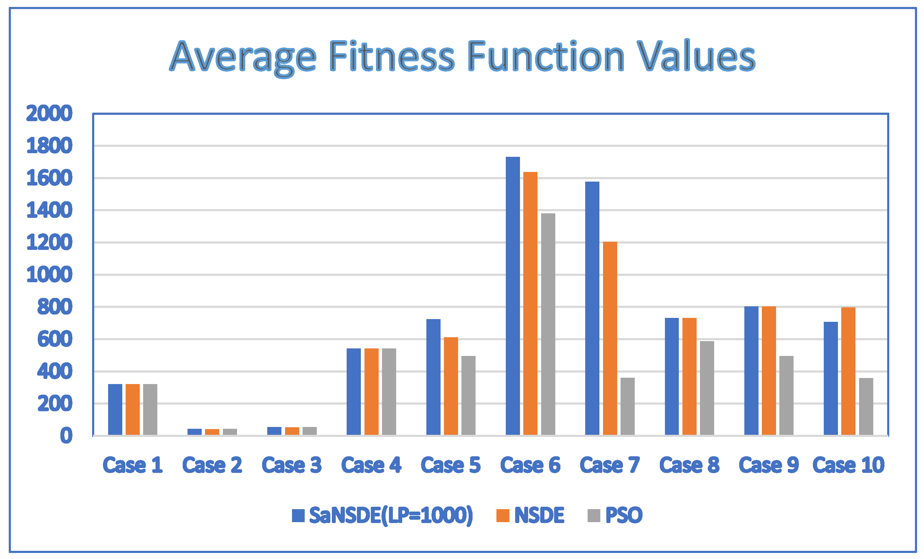
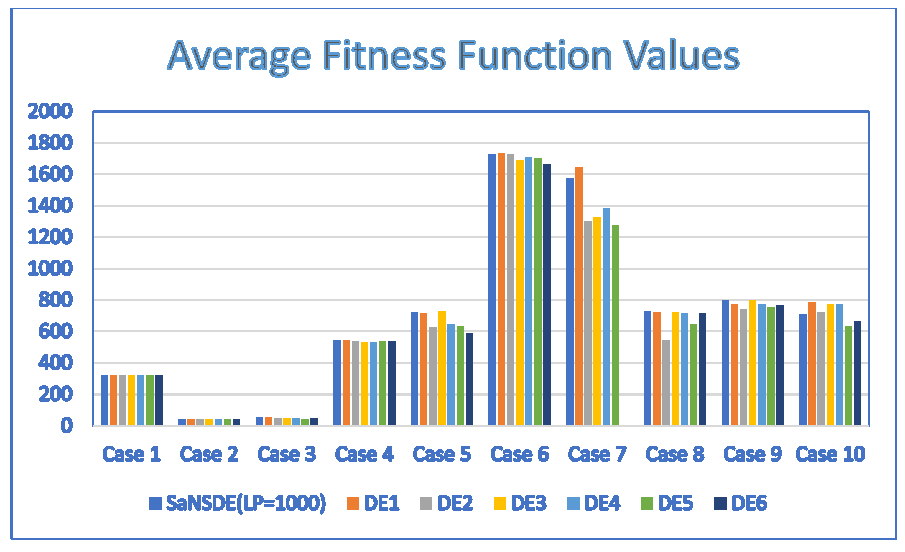
Table 7 and Table 8 show the results for the population size = 30, obtained by applying the SaNSDE algorithm, a variant of the neighborhood search-based DE (NSDE) algorithm, the PSO algorithm and six standard DE algorithms. The average fitness function values in Table 7 and Table 8 are shown in the bar charts of Figure 7 and Figure 8, respectively.

Table 7.
Fitness function values for discrete NSDE, NSDE and PSO with population size = 30.

Table 8.
Average fitness function values for DE1, DE2, DE3, DE4, DE5 and DE6 with = 30.

Figure 7.
Average fitness function values for discrete SaNSDE ( = 1000), NSDE and PSO with NP = 30.

Figure 8.
Average fitness function values for SaNSDE ( = 1000), DE1, DE2, DE3, DE4, DE5 and DE6 with NP = 30.
In terms of performance, the results of Table 7 indicate that the SaNSDE algorithm either outperforms or performs as well as the NSDE algorithm and PSO algorithm in all instances. The results of Table 8 indicate that the SaNSDE algorithm either outperforms or performs as well as the six standard DE algorithms for most instances, with the exceptions of Case 5 and Case 7. The number of best solutions found by the SaNSDE algorithm, the NSDE algorithm, the PSO algorithm, DE1 algorithm, DE2 algorithm, DE3 algorithm, DE4 algorithm, DE5 algorithm and DE6 algorithm are 8, 4, 3, 7, 3, 2, 1, 1 and 2, respectively. Therefore, in terms of the number of best solutions found, the SaNSDE algorithm outperforms the other algorithms.
Table 9 and Table 10 show the results for the population size = 50, obtained by applying the SaNSDE algorithm, a variant of the neighborhood search-based DE (NSDE) algorithm, the PSO algorithm and six standard DE algorithms. The average fitness function values in Table 9 and Table 10 are shown in the bar charts of Figure 9 and Figure 10, respectively.

Table 9.
Fitness function values for discrete NSDE, NSDE and PSO with population size = 50.

Table 10.
Average fitness function values for DE1, DE2, DE3, DE4, DE5 and DE6 with = 50.
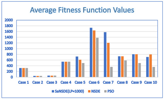
Figure 9.
Average fitness function values for discrete SaNSDE ( = 1000), NSDE and PSO with NP = 50.
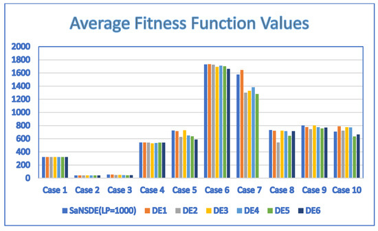
Figure 10.
Average fitness function values for SaNSDE ( = 1000), DE1, DE2, DE3, DE4, DE5 and DE6 with NP = 50.
In terms of performance, the results of Table 9 indicate that the SaNSDE algorithm either outperforms or performs as well as the NSDE algorithm and PSO algorithm for all instances. The results of Table 10 indicate that the SaNSDE algorithm either outperforms or performs as well as the six standard DE algorithms in most instances, with the exceptions of Case 5, Case 6 and Case 7. The number of best solutions found by the SaNSDE algorithm, the NSDE algorithm, the PSO algorithm, DE1 algorithm, DE2 algorithm, DE3 algorithm, DE4 algorithm, DE5 algorithm and DE6 algorithm are 7, 3, 4, 5, 1, 4, 2, 2 and 1, respectively. Therefore, in terms of the number of best solutions found, the SaNSDE algorithm outperforms the other algorithms.
4.3. Influence of the LP Parameter on the Performance/Efficiency
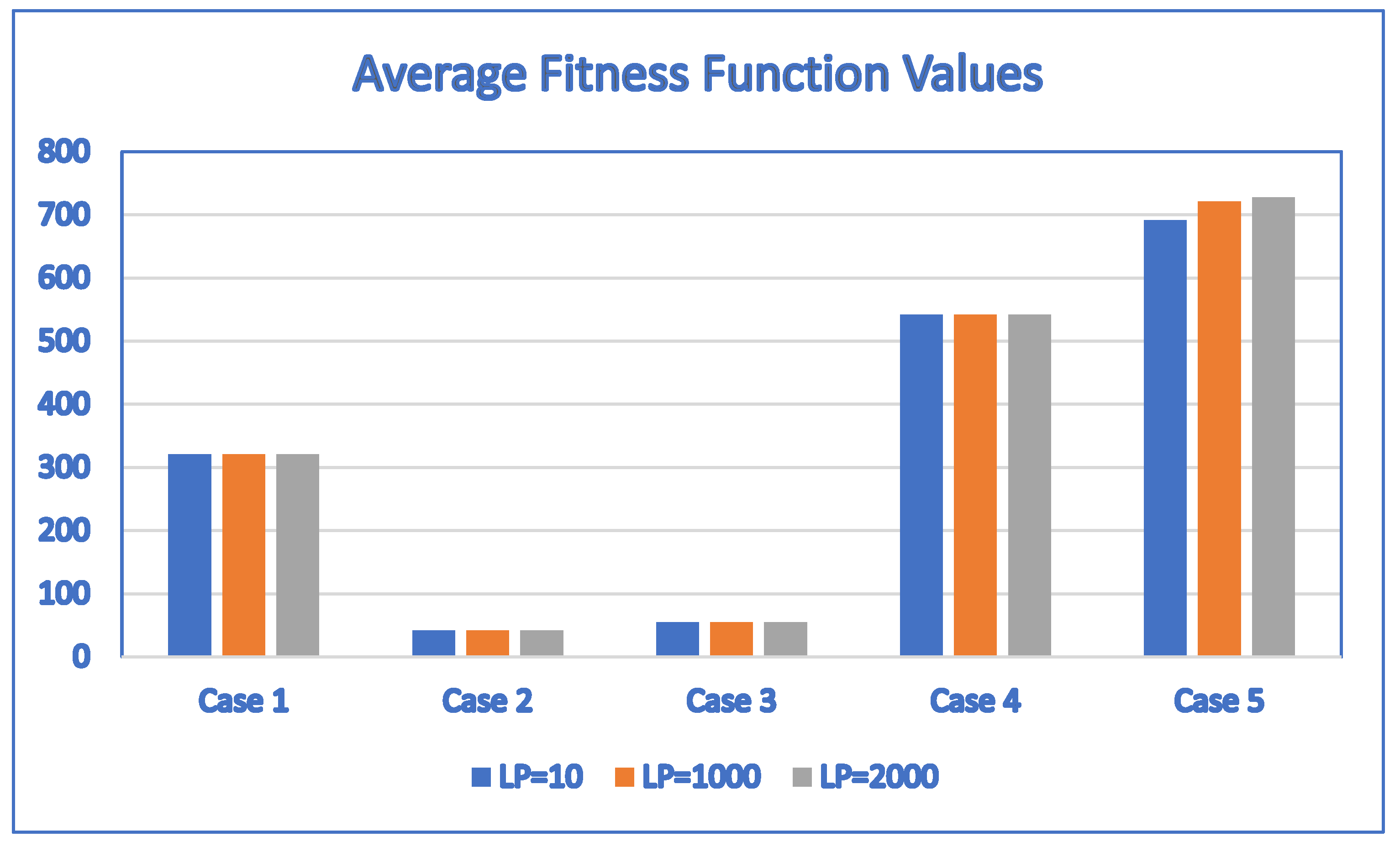
The learning period parameter of the SaNSDE algorithm proposed in Section 3.2 may have an influence on its performance and efficiency. An important issue to study is whether the learning period parameter has a significant influence on performance and efficiency. To understand the effects of the learning period parameter, we perform three series of experiments by setting the learning period parameter, , to 10, 1000 and 2000, respectively, and then analyzing the outcomes by comparing performance and efficiency. The results of the series of experiments are based on the same set of test cases. The results are summarized in Table 11. The average fitness function values in Table 10 are shown in the bar charts of Figure 11 and Figure 12, respectively.

Table 11.
Average fitness values and average number of generations for SaNSDE with algorithmic parameter = 10, 1000 and 2000.
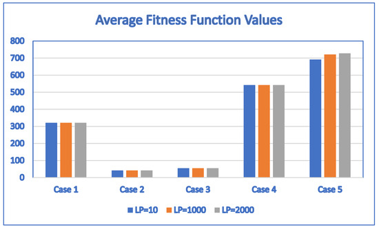
Figure 11.
The average fitness function values obtained by SaNSDE with = 10, 1000 and 2000 for Case 1, Case 2, Case 3, Case 4 and Case 5.
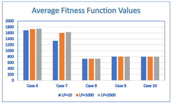
Figure 12.
The average fitness function values obtained by SaNSDE with LP = 10, 1000 and 2000 for Case 6, Case 7, Case 8, Case 9 and Case 10.
According to Table 11, the average fitness values are the same for Case 1 through Case 4, Case 9 and Case 10 regardless of whether the learning period parameter is set to 10, 1000 or 2000. This indicates that the proposed SaNSDE algorithm is not sensitive to the learning period parameter for Case 1 through Case 4, Case 9 and Case 10.
For Case 5, the average fitness values depend on the values of . The maximum average fitness value is 727.66, which is obtained by setting = 2000, and the minimum average fitness value is 691.48, which is obtained by setting = 10. The difference between the maximum and the minimum average fitness values is (727.66 − 691.48)/691.48 = 5.2322%.
For Case 6, the average fitness values depend on the values of . The maximum average fitness value is 1743.7, which is obtained by setting = 2000, and the minimum average fitness value is 1685.8, which is obtained by setting = 10. The difference between the maximum and the minimum average fitness values is (1743.7 − 1685.8)/1685.8 = 3.4345%.
For Case 7, the average fitness values depend on the values of . The maximum average fitness value is 1629.2, which is obtained by setting = 2000, and the minimum average fitness value is 1334.1, which is obtained by setting = 10. The difference between the maximum and the minimum average fitness values is (1629.2 − 1334.1)/1334.1 = 22.1197%.
For Case 8, the average fitness values depend on the values of . The maximum average fitness value is 731, which is obtained by setting = 1000 or 2000, and the minimum average fitness value is 728.8, which is obtained by setting = 10. The difference between the maximum and the minimum average fitness values is (731 − 728.8)/728.8 = 0.3018%.
The above analysis indicates that the sensitivity to the average fitness values obtained by the proposed SaNSDE algorithm is less than 5% for most cases, with the exception of Case 7. Another observation of the results is that should be large enough to obtain better average fitness values.
4.4. Influence of Population Size on Performance/Efficiency
To study the influence of population size on the performance of the SaNSDE algorithm proposed in Section 3.2, we perform three series of experiments for all test cases for = 10, 30 and 50. The results of these experiments are summarized in Table 12. The average fitness function values of Table 12 are shown in the bar charts of Figure 13 and Figure 14, respectively.

Table 12.
Average fitness values and average number of generations for SaNSDE with algorithmic parameter = 10, 30 and 50.
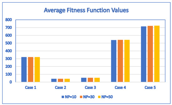
Figure 13.
The average fitness function values obtained by SaNSDE with = 10, 30 and 50 for Case 1, Case 2, Case 3, Case 4 and Case 5.
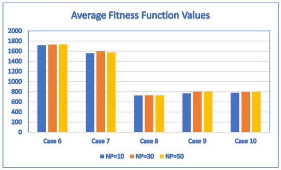
Figure 14.
The average fitness function values obtained by SaNSDE with = 10, 30 and 50 for Case 6, Case 7, Case 8, Case 9 and Case 10.
The results show that the average fitness values of Case 1, Case 2 and Case 3 are the same. For Case 4, Case 5, Case 6, Case 7, Case 8, Case 9 and Case 10, the differences between the average fitness values for = 10, 30 and 50 are small in terms of percentage based on the following analysis of the results. This indicates that the proposed SaNSDE algorithm is not sensitive to population size.
For other test cases, although the average fitness values are not always the same, they are close. For Case 4, the maximum average fitness value is 542.2, which is obtained by setting = 30 or = 50, and the minimum average fitness value is 539, which is obtained by setting = 10. The difference between the maximum and the minimum average fitness values is (542.2 − 539)/539 = 0.5936%.
For Case 5, the maximum average fitness value is 724.02, which is obtained by setting = 50, and the minimum average fitness value is 715.08, which is obtained by setting = 10. The difference between the maximum and the minimum average fitness values is (724.02 − 715.08)/715.08 = 1.2502%.
For Case 6, the maximum average fitness value is 1730.5, which is obtained by setting = 50, and the minimum average fitness value is 1717, which is obtained by setting = 10. The difference between the maximum and the minimum average fitness values is (1730.5 − 1717)/1717 = 0.7862%.
For Case 7, the maximum average fitness value is 1598.3, which is obtained by setting = 30, and the minimum average fitness value is 1557.9, which is obtained by setting = 10. The difference between the maximum and the minimum average fitness values is (1598.3 − 1557.9)/1557.9 = 2.5932%.
For Case 8, the maximum average fitness value is 731, which is obtained by setting = 30 or = 50, and the minimum average fitness value is 726.9, which is obtained by setting = 10. The difference between the maximum and the minimum average fitness values is (731 − 726.9)/726.9 = 0.5640%.
For Case 9, the maximum average fitness value is 802, which is obtained by setting = 30 or = 50, and the minimum average fitness value is 768.8, which is obtained by setting = 10. The difference between the maximum and the minimum average fitness values is (802 − 768.8)/768.8 = 4.3184%.
For Case 10, the maximum average fitness value is 797, which is obtained by setting = 30 or = 50, and the minimum average fitness value is 780.1, which is obtained by setting = 10. The difference between the maximum and the minimum average fitness values is (797 − 780.1)/780.1 = 2.1663%.
The above results show that the difference between the maximum average fitness value and the minimum average fitness value is less than 2% for most test cases, with the exceptions of Case 7, Case 9 and Case 10. The difference between the maximum average fitness value and the minimum average fitness value is less than 4.5% for Case 7, Case 9 and Case 10. The results of the experiments show that the proposed algorithm is not sensitive to population size.
4.5. Statistical Significance of the Results
To illustrate the benefits and statistical significance of the results obtained by the proposed algorithm, let us take the setting with = 1000 as an example.
The standard deviation of the fitness function values obtained by the proposed algorithm and all the algorithms compared in this study are listed in Table 13 and Table 14 for = 10 and = 1000. The standard deviation of the fitness function values obtained by the proposed algorithm is smaller than those of the other algorithms compared in this study with only a few exceptions. This indicates that the variation in the fitness function values obtained by the proposed algorithm is smaller than those of other algorithms, and the fitness function values are clustered tightly around the mean of the fitness function values. Therefore, this shows that the proposed algorithm is more robust than the compared algorithms in this study.

Table 13.
Standard deviation of fitness function values for discrete SaNSDE, NSDE and PSO with population size = 10 and = 1000.

Table 14.
Standard deviation of fitness function values for DE1, DE2, DE3, DE4, DE5 and DE6 with = 10 and = 1000.
The standard deviation of the fitness function values obtained by the proposed algorithm and all the algorithms compared in this study are listed in Table 15 and Table 16 for NP = 30 and LP = 1000. Again, the standard deviation of the fitness function values obtained by the proposed algorithm is smaller than those of the other algorithms compared in this study with only a few exceptions. In particular, the standard deviation of the fitness function values obtained by the proposed algorithm is smaller than those of all the compared DE algorithms in this study. Therefore, this shows that the proposed algorithm is more robust than the compared algorithms in this study.

Table 15.
Standard deviation of fitness function values for discrete SaNSDE, NSDE and PSO with population size = 30 and = 1000.

Table 16.
Standard deviation of fitness function values for DE1, DE2, DE3, DE4, DE5 and DE6 with = 30 and = 1000.
The standard deviation of the fitness function values obtained by the proposed algorithm and all the algorithms compared in this study are listed in Table 17 and Table 18 for = 50 and = 1000. Again, the standard deviation of the fitness function values obtained by the proposed algorithm is smaller than those of the other algorithms compared in this study with only a few exceptions. In particular, the standard deviation of the fitness function values obtained by the proposed algorithm is smaller than those of all DE algorithms. Therefore, this shows that the proposed algorithm is more robust than the other algorithms compared in this study.

Table 17.
Standard deviation of fitness function values for discrete SaNSDE, NSDE and PSO with population size = 50 and = 1000.

Table 18.
Standard deviation of fitness function values for DE1, DE2, DE3, DE4, DE5 and DE6 with = 50 and = 1000.
The above results show that the proposed algorithm can ensure that the variation in solutions is smaller than in the other algorithms compared in this study with only a few exceptions regardless of the population size.
5. Discussion
In this study, we proposed a SaNSDE algorithm for planning processes in sustainable CPSs and conducted experiments to illustrate its effectiveness and properties. These included a comparative study with other competitive algorithms to illustrate the effectiveness of the proposed self-adaptive algorithm. In addition, we studied the sensitivity of the proposed self-adaptive algorithm with respect to algorithmic parameters, including the learning period parameter, , and the population size parameter, .
Several other algorithms, including the PSO algorithm, six standard DE algorithms and a variant of the neighborhood search-based DE algorithm, were applied to solve ten instances. The results obtained by these algorithms were compared with those obtained by applying the SaNSDE algorithm to the same set of instances. Three series of experiments were conducted based on a small population size of 10, a moderate population size of 30 and a larger population size of 50 in this study. In terms of the number of best solutions found, the SaNSDE algorithm outperformed the other algorithms regardless of whether the population size was set to 10, 30 or 50.
To study the impacts of the learning period parameter, , on the performance, we conducted several experiments by changing the values of . To understand the effects of the learning period parameter, we performed three series of experiments based on the same set of test cases by setting the learning period parameter, , to 10, 1000 and 2000, respectively. We analyzed the outcomes by comparing performance. The results indicate that the proposed SaNSDE algorithm is not sensitive to the learning period parameter for Case 1 through Case 4, Case 9 and Case 10. The sensitivity of the average fitness values obtained by the proposed SaNSDE algorithm is less than 5% for most cases, with the exception of Case 7. Another observation of the results is that should be large enough to obtain better average fitness values. If the parameter is too small, it is difficult to learn the best strategy within the learning period. As a result, the probability of creating a potential candidate solution using the best strategy will be low. In this case, the performance will be degraded. If is big enough, the probability of learning the best strategy within the learning period will be higher. Hence the probability of creating a potential candidate solution by learning the best strategy will be higher. In this case, the performance tends to be improved. The results presented in Section 4.3 indicate that for the algorithm to perform better, must be large enough. This poses an interesting and challenging future research direction to prove that the performance can be improved by setting to a large value through theoretical analysis.
To study the effects of population size on the performance of the proposed algorithm, we performed three series of experiments for all test cases for = 10, 30 and 50. The results show that the average fitness values of Case 1, Case 2 and Case 3 are the same. For Case 4 through Case 10, the differences between the average fitness values for = 10, 30 and 50 are small in terms of percentage. This indicates that the proposed SaNSDE algorithm is not sensitive to population size. In summary, the above results show that the proposed algorithm can ensure that the variation in solutions is smaller than in the other algorithms compared in this study with only a few exceptions regardless of the population size.
There are two problems formulated in this paper. The first problem formulation is for a general planning problem, whereas the second one is a special case of the first problem formulation for a sequential processes planning problem. As sequential processes are found in many production systems, we first started with the development of an effective problem solver for the second problem formulation and verification for sequential processes in this paper. As the solution algorithms take the same form, with the exception of the fitness function, the solution algorithm for the second problem (for sequential processes) can be tailored for other types of production processes. This includes the development of efficient methods to compute a penalty due to the violation of constraints , a penalty due to the violation of constraints and a penalty due to the violation of constraints . Based on the discussion above, the proposed algorithm has the potential to be extended to deal with other types of production processes. Tailoring the proposed algorithm to deal with other types of production processes and studying its effectiveness are nontrivial interesting future research directions.
Due to the need to verify the proposed algorithm, many examples (test cases) were created for the verification of the proposed algorithm. The characteristics of these examples are similar to the ones in real situations. Our previous experiences with other problems showed that if the parameters used by the proposed SaNSDE algorithm worked for many instances of the test cases, these parameters usually worked well for real application scenarios. In addition, the results of the experiments conducted in this study show that the performance of the proposed algorithm is insensitive with respect to algorithmic parameters. Therefore, the parameters used by the proposed SaNSDE algorithm are expected to work for real application scenarios. In summary, the preliminary results of this study pave the way for solving the real planning problem in sustainable CPSs by applying the proposed algorithm. Testing whether the parameters used in the experiments of this study can work for real data is an interesting future research direction.
6. Conclusions
Although CPSs provide a flexible architecture for enterprises to accommodate changes in processes, resources and demand, the development of a methodology to realize the flexibility advantage of CPSs is required to plan its processes to meet the goals of production in terms of time, energy consumption and constraints. We formulated a general optimization problem for planning processes in sustainable CPSs, taking into account the factors of time, energy consumption and related constraints. We proposed a solution methodology to solve this problem based on a self-adaptive Differential Evolution approach with a neighborhood search mechanism. To verify the proposed methodology, we applied it to processes with sequential workflows. We tailored the problem formulation of the proposed general framework for processes with sequential structures. We studied the effectiveness of the proposed solution algorithm in terms of performance and robustness.
We assessed the performance and robustness of this approach by performing experiments for several cases. By comparing the results of the experiments, it was indicated that the proposed method outperforms several other algorithms in the literature in terms of the number of best solutions found regardless of the population size. To illustrate the robustness of the proposed self-adaptive algorithm, experiments with different settings of algorithmic parameters were conducted. Two parameters were considered in the experiments to assess the robustness of the proposed algorithm, including population size and learning period. The population size was set to 10, 30 or 50 for all the algorithms used in the experiments of this study. Three series of experiments were performed for all test cases for = 10, 30 and 50. The results show that the average fitness values of three of the test cases are the same and the differences between the average fitness values are small in terms of percentage. This indicates that the proposed SaNSDE algorithm is not sensitive to population size. That is, the proposed self-adaptive algorithm is robust with respect to population size. To study the effects of the learning period parameter, we performed three series of experiments by setting the learning period parameter, , to 10, 1000 and 2000, respectively, and then analyzed the outcomes by comparing performance and efficiency. The results of the series of experiments were obtained based on the same set of test cases. The results show that the sensitivity of the average fitness values obtained by the proposed SaNSDE algorithm is less than 5% for most cases with only one exception. This indicates that the proposed SaNSDE algorithm is robust with respect to the learning period parameter. The preliminary results presented in this paper show that combining a self-adaptive mechanism with neighborhood search in the Differential Evolution approach leads to an effective algorithm in comparison with other competitive algorithms. To apply the proposed algorithm in industrial settings, a further study on the scalability of the proposed algorithm with respect to the problem size needs to be conducted.
In this paper, we applied the proposed method to study the effectiveness of different evolutionary algorithms for sequential production processes. As we limited our scope to sequential processes in this paper to illustrate the solution methodology, the computational experiences of these results hold for sequential processes. However, the application of the proposed method is not limited to sequential production processes. The general problem formulation for planning processes in CPSs proposed in this paper can be applied to a variety of production processes. Based on the reasoning in the Discussion section of this paper, the proposed algorithm has the potential to be extended to deal with other types of production processes. Tailoring the proposed algorithm to deal with other types of production processes and studying its effectiveness are nontrivial interesting future research directions. Another future research direction is to develop other evolutionary algorithms and compare their effectiveness with respect to the algorithms studied in this paper.
Funding
This research was supported in part by the National Science and Technology Council, Taiwan, under grant NSTC 111-2410-H-324-003.
Institutional Review Board Statement
Not applicable.
Informed Consent Statement
Not applicable.
Data Availability Statement
The original data presented in the study are openly available in [Planning_CPS] at [https://drive.google.com/drive/folders/1_5bMvhjvVhTDN0yunbFNQ4HasaICu8b4?usp=sharing] (accessed on 29 June 2024).
Conflicts of Interest
The author declares no conflicts of interest.
References
- Lu, Y. Industry 4.0: A survey on technologies, applications and open research issues. J. Ind. Inf. Integr. 2017, 6, 1–10. [Google Scholar] [CrossRef]
- Monostori, L.; Kádár, B.; Bauernhansl, T.; Kondoh, S.; Kumara, S.; Reinhart, G.; Sauer, O.; Schuh, G.; Sihn, W.; Ueda, K. Cyber-physical systems in manufacturing. CIRP Ann. 2016, 65, 621–641. [Google Scholar] [CrossRef]
- Hsieh, F.-S. A Theoretical Foundation for Context-Aware Cyber-Physical Production Systems. Appl. Sci. 2022, 12, 5129. [Google Scholar] [CrossRef]
- Cheng, T.; Liu, Z.; Zhang, L. Software-Defined Modeling Method of Cyber-Physical System Driven by Big Data. In Proceedings of the 2021 IEEE 12th International Conference on Software Engineering and Service Science (ICSESS), Beijing, China, 20–22 August 2021; pp. 211–214. [Google Scholar]
- Brovkova, M.B.; Pylskij, V.A.; Ushakova, O.V.; Torgashova, O.Y.; Martynov, V.V. Approaches to measuring and modeling the computing part of a cyber physical monitoring system for industrial production, taking into account modularity and hybridization. In Proceedings of the 2021 5th Scientific School Dynamics of Complex Networks and their Applications (DCNA), Kaliningrad, Russia, 13–15 September 2021; pp. 49–52. [Google Scholar]
- Khrueangsakun, S.; Nuratch, S.; Boonpramuk, P. Design and Development of Cyber Physical System for Real-Time Web-based Visualization and Control of Robot Arm. In Proceedings of the 2020 5th International Conference on Control and Robotics Engineering (ICCRE), Osaka, Japan, 24–26 April 2020; pp. 11–14. [Google Scholar]
- Kruglova, T.; Schmelev, I.; Sushkov, I.; Filatov, R. Cyber-physical System of the Mobile Robot’s Optimal Trajectory Planning with taking into account Electric Motors Deterioration. In Proceedings of the 2019 International Multi-Conference on Industrial Engineering and Modern Technologies (FarEastCon), Vladivostok, Russia, 1–4 October 2019; pp. 1–5. [Google Scholar]
- Su, R.; Shen, C.; Huang, S.; Cui, X.; Xu, J.; Lei, M. Preventive control and routing planning of cyber-physical system based on master-slave game. In Proceedings of the Tsinghua University-IET Electrical Engineering Academic Forum: Constructing Green and Sustainable Energy System (2021), Beijing, China, 15–16 May 2021; pp. 52–60. [Google Scholar]
- Zhao, D.; Liu, C.; Xu, G.; Ding, Z.; Peng, H.; Yu, J.; Han, J. A security enhancement model based on switching edge strategy in interdependent heterogeneous cyber-physical systems. China Commun. 2022, 19, 158–173. [Google Scholar] [CrossRef]
- Hsieh, F.S. A Dynamic Context-Aware Workflow Management Scheme for Cyber-Physical Systems Based on Multi-Agent System Architecture. Appl. Sci. 2021, 11, 2030. [Google Scholar] [CrossRef]
- Hsieh, F.-S. An Efficient Method to Assess Resilience and Robustness Properties of a Class of Cyber-Physical Production Systems. Symmetry 2022, 14, 2327. [Google Scholar] [CrossRef]
- Transforming Our World: The 2030 Agenda for Sustainable Development. Available online: https://sdgs.un.org/2030agenda (accessed on 20 June 2024).
- Thiede, S. Environmental Sustainability of Cyber Physical Production Systems. Procedia CIRP 2018, 69, 644–649. [Google Scholar] [CrossRef]
- Andronie, M.; Lăzăroiu, G.; Iatagan, M.; Hurloiu, I.; Dijmărescu, I. Sustainable Cyber-Physical Production Systems in Big Data-Driven Smart Urban Economy: A Systematic Literature Review. Sustainability 2021, 13, 751. [Google Scholar] [CrossRef]
- Andronie, M.; Lăzăroiu, G.; Ștefănescu, R.; Uță, C.; Dijmărescu, I. Sustainable, Smart, and Sensing Technologies for Cyber-Physical Manufacturing Systems: A Systematic Literature Review. Sustainability 2021, 13, 5495. [Google Scholar] [CrossRef]
- Restrepo, L.; Aguilar, J.; Toro, M.; Suescún, E. A sustainable-development approach for self-adaptive cyber–physical system’s life cycle: A systematic mapping study. J. Syst. Softw. 2021, 180, 111010. [Google Scholar] [CrossRef]
- Chantem, T.; Guan, N.; Liu, D. Sustainable embedded software and systems. Sustain. Comput. Inform. Syst. 2019, 22, 152–154. [Google Scholar] [CrossRef]
- Sihag, N.; Sangwan, K.S. A systematic literature review on machine tool energy consumption. J. Clean. Prod. 2020, 275, 123125. [Google Scholar] [CrossRef]
- Zhou, L.; Li, J.; Li, F.; Meng, Q.; Li, J.; Xu, X. Energy consumption model and energy efficiency of machine tools: A comprehensive literature review. J. Clean. Prod. 2016, 112, 3721–3734. [Google Scholar] [CrossRef]
- Guo, Z.L.; Zhang, Y.; Liu, S.; Wang, X.V.; Wang, L. Exploring self-organization and self-adaption for smart manufacturing complex networks. Front. Eng. Manag. 2023, 10, 206–222. [Google Scholar] [CrossRef]
- Dias-Ferreira, J.; Ribeiro, L.; Akillioglu, H.; Neves, P.; Onori, M. BIOSOARM: A bio-inspired self-organising architecture for manufacturing cyber-physical shopfloors. J. Intell. Manuf. 2018, 29, 1659–1682. [Google Scholar] [CrossRef]
- Estrada-Jimenez, L.A.; Pulikottil, T.; Nikghadam-Hojjati, S.; Barata, J. Self-Organization in Smart Manufacturing—Background, Systematic Review, Challenges and Outlook. IEEE Access 2023, 11, 10107–10136. [Google Scholar] [CrossRef]
- Zeadally, S.; Sanislav, T.; Mois, G. Self-adaptation techniques in cyber-physical systems (CPSs). IEEE Access 2019, 7, 171126–171139. [Google Scholar] [CrossRef]
- Lee, J.; Bagheri, B.; Kao, H.A. A Cyber-Physical Systems Architecture for Industry 4.0-Based Manufacturing Systems. Manuf. Lett. 2015, 3, 18–23. [Google Scholar] [CrossRef]
- Parente, M.; Figueira, G.; Amorim, P.; Marques, A. Production scheduling in the context of Industry 4.0: Review and trends. Int. J. Prod. Res. 2020, 58, 5401–5431. [Google Scholar] [CrossRef]
- Prashar, A.; Tortorella, G.L.; Fogliatto, F.S. Production scheduling in Industry 4.0: Morphological analysis of the literature and future research agenda. J. Manuf. Syst. 2022, 65, 33–43. [Google Scholar] [CrossRef]
- Rossit, D.A.; Tohmé, F.; Frutos, M. Production planning and scheduling in Cyber-Physical Production Systems: A review. Int. J. Comput. Integr. Manuf. 2019, 32, 385–395. [Google Scholar] [CrossRef]
- Meissner, H.; Aurich, J.C. Implications of Cyber-Physical Production Systems on Integrated Process Planning and Scheduling. Procedia Manuf. 2019, 28, 167–173. [Google Scholar] [CrossRef]
- Seitz, K.-F.; Nyhuis, P. Cyber-Physical Production Systems Combined with Logistic Models—A Learning Factory Concept for an Improved Production Planning and Control. Procedia CIRP 2015, 32, 92–97. [Google Scholar] [CrossRef]
- Rogalla, A.; Niggemann, O. Automated process planning for cyber-physical production systems. In Proceedings of the 2017 22nd IEEE International Conference on Emerging Technologies and Factory Automation (ETFA), Limassol, Cyprus, 12–15 September 2017; pp. 1–8. [Google Scholar] [CrossRef]
- Murata, T. Petri nets: Properties, analysis and applications. Proc. IEEE 1989, 77, 541–580. [Google Scholar] [CrossRef]
- Tan, B.Q.; Yu, C.; Kang, K.; Zhong, R.Y.; Li, M.; Huang, G.Q. Transportation Service Procurement Auctions in Cyber-Physical Internet. IFAC-PapersOnLine 2023, 56, 7626–7631. [Google Scholar] [CrossRef]
- Kong, X.T.R.; Kang, K.; Zhong, R.Y.; Luo, H.; Xu, S.X. Cyber physical system-enabled on-demand logistics trading. Int. J. Prod. Econ. 2021, 233, 108005. [Google Scholar] [CrossRef]
- Yu, K.; Yan, P.; Kong, X.T.R.; Yang, L.; Levner, E. Sequential auction for cloud manufacturing resource trading: A deep reinforcement learning approach to the lot-sizing problem. Comput. Ind. Eng. 2024, 188, 109862. [Google Scholar] [CrossRef]
- Krämer, L.; Ahlbäumer, R.; Roidl, M. Two-Stage Market-Based Task Allocation for Blockchain-Based Cyber-Physical Production Systems. In Proceedings of the 2022 IEEE International Conference on Blockchain (Blockchain), Espoo, Finland, 22–25 August 2022; pp. 282–289. [Google Scholar]
- Nejati, S. Testing Cyber-Physical Systems via Evolutionary Algorithms and Machine Learning. In Proceedings of the 2019 IEEE/ACM 12th International Workshop on Search-Based Software Testing (SBST), Montreal, QC, Canada, 26–27 May 2019; p. 1. [Google Scholar]
- Chen, R.; Shen, H.; Lai, Y. A Metaheuristic Optimization Algorithm for energy efficiency in Digital Twins. Internet Things Cyber Phys. Syst. 2022, 2, 159–169. [Google Scholar] [CrossRef]
- Shah, P.; Sekhar, R.; Kulkarni, A.J.; Siarry, P. (Eds.) Metaheuristic Algorithms in Industry 4.0; Taylor & Francis: London, UK, 2021. [Google Scholar] [CrossRef]
- Gong, H.; Li, R.; An, J.; Chen, W.; Li, K. Scheduling Algorithms of Flat Semi-Dormant Multicontrollers for a Cyber-Physical System. IEEE Trans. Ind. Inform. 2017, 13, 1665–1680. [Google Scholar] [CrossRef]
- Xu, X.; Mo, R.; Yin, X.; Khosravi, M.R.; Aghaei, F.; Chang, V.; Li, G. PDM: Privacy-Aware Deployment of Machine-Learning Applications for Industrial Cyber–Physical Cloud Systems. IEEE Trans. Ind. Inform. 2021, 17, 5819–5828. [Google Scholar] [CrossRef]
- Hsieh, F.S. Trust-Based Recommendation for Shared Mobility Systems Based on a Discrete Self-Adaptive Neighborhood Search Differential Evolution Algorithm. Electronics 2022, 11, 776. [Google Scholar] [CrossRef]
- Price, K.; Storn, R.; Lampinen, J. Differential Evolution: A Practical Approach to Global Optimization; Springer: Berlin/Heidelberg, Germany, 2005. [Google Scholar]
- Souza, I.P.; Boeres, M.C.S.; Moraes, R.E.N. A robust algorithm based on Differential Evolution with local search for the Capacitated Vehicle Routing Problem. Swarm Evol. Comput. 2023, 77, 101245. [Google Scholar] [CrossRef]
- Caraffini, F.; Kononova, A.V.; Corne, D. Infeasibility and structural bias in differential evolution. Inf. Sci. 2019, 496, 161–179. [Google Scholar] [CrossRef]
- Yang, Z.; He, J.; Yao, X. Making a difference to differential evolution. In Advances in Metaheuristics for Hard Optimization; Michalewicz, Z., Siarry, P., Eds.; Springer: Berlin/Heidelberg, Germany, 2007; pp. 397–414. [Google Scholar]
- Hsieh, F.-S. Applying “Two Heads Are Better Than One” Human Intelligence to Develop Self-Adaptive Algorithms for Ridesharing Recommendation Systems. Electronics 2024, 13, 2241. [Google Scholar] [CrossRef]
- Deb, K. An efficient constraint handling method for genetic algorithms. Comput. Methods Appl. Mech. Eng. 2000, 186, 311–338. [Google Scholar] [CrossRef]
- Hsieh, F.-S. Collaboration of Machines and Robots in Cyber Physical Systems based on Evolutionary Computation Approach. In Proceedings of the 2019 International Joint Conference on Neural Networks (IJCNN), Budapest, Hungary, 14–19 July 2019; pp. 1–8. [Google Scholar]
- Hsieh, F.-S. Neighborhood Search for Process Resource Configuration in Cyber Physical Systems. In Proceedings of the 2021 IEEE 12th Annual Information Technology, Electronics and Mobile Communication Conference (IEMCON), Vancouver, BC, Canada, 27–30 October 2021; pp. 877–881. [Google Scholar]
- Hsieh, F.-S. Comparison of a Hybrid Firefly–Particle Swarm Optimization Algorithm with Six Hybrid Firefly–Differential Evolution Algorithms and an Effective Cost-Saving Allocation Method for Ridesharing Recommendation Systems. Electronics 2024, 13, 324. [Google Scholar] [CrossRef]
- Hsieh, F.-S. Development and Comparison of Ten Differential-Evolution and Particle Swarm-Optimization Based Algorithms for Discount-Guaranteed Ridesharing Systems. Appl. Sci. 2022, 12, 9544. [Google Scholar] [CrossRef]
Disclaimer/Publisher’s Note: The statements, opinions and data contained in all publications are solely those of the individual author(s) and contributor(s) and not of MDPI and/or the editor(s). MDPI and/or the editor(s) disclaim responsibility for any injury to people or property resulting from any ideas, methods, instructions or products referred to in the content. |
© 2024 by the author. Licensee MDPI, Basel, Switzerland. This article is an open access article distributed under the terms and conditions of the Creative Commons Attribution (CC BY) license (https://creativecommons.org/licenses/by/4.0/).


