Feasibility of Identifying Shale Sweet Spots by Downhole Microseismic Imaging

Abstract

Several studies suggest that shale sweet spots are likely associated with a low Poisson’s ratio in the shale layer. Compared with conventional geophysical techniques with active seismic data, it is straightforward and cost-effective to delineate the distribution of 3D Poisson’s ratios using microseismic data. In this study, an alternating method is proposed to determine microseismic event locations, 3D P-wave velocity, and Poisson’s ratio models with data recorded from downhole monitoring arrays. The method combines the improved 3D traveltime tomography, which inverts P and S arrivals for 3D P-wave velocity and Poisson’s ratio structures simultaneously, and a 3D grid search approach for event locations in an iterative fashion. The traveltime tomography directly inverts the Poisson’s ratio structure instead of calculating the Poisson’s ratios from P- and S-wave velocities (i.e., Vp and Vs) that are inverted by conventional traveltime tomography separately. The synthetic results and analysis suggest that the proposed method recovers the true Poisson’s ratio model reasonably. Additionally, we apply the method to a field dataset, which indicates that it may help delineate the reservoir structure and identify potential shale sweet spots.

1. Introduction

The sweet spot of geological formations is the concurrence of several favorable geologic contents such as fracturing, thermal history, gas content, reservoir thickness, or matrix rock properties, and, economically, areas that are most likely to be the developed parts of continuous accumulation [1]. Norton and Maxwell [2] defined that a shale sweet spot is a region likely to yield high gas production, associated with a low Poisson’s ratio. With an increase in light hydrocarbon saturation, the compressional wave velocity decreases and shear wave velocity increases, thereby resulting in a low velocity ratio (Vp/Vs ratio) or Poisson’s ratio. By analyzing Poisson’s ratio distributions derived from conventional seismic processing of surface seismic data, they identified potential high-yield areas in shale formations.

The Poisson’s ratio, or the Vp/Vs ratio, serves as a critical indicator of reservoir lithology and fluid properties [3,4]. Widely utilized in active seismic exploration, the Vp/Vs ratio facilitates hydrocarbon identification and stratigraphic interpretations from reflection seismic data [5,6]. Anderson and Lines [7] reviewed three methods for estimating the Vp/Vs ratio to elucidate rock properties from seismic data: AVO analysis coupled with the post-stack inversion of AVO attributes [8], the prestack inversion of P-wave gathers directly to impedances [9], and the joint prestack inversion of P-wave and converted wave data to impedances [9]. Despite the effectiveness of these techniques in identifying sweet spots within reservoirs, their high cost and lengthy processing times restrict routine use [10,11].

In passive seismology, 3D passive seismic traveltime tomography is recognized as a crucial technique for understanding seismotectonics and seismogenic processes across extensive regions [12,13,14]. The methodology has been comprehensively reviewed by experts such as Thurber [15], Kissling [16], and Iyer and Hirahara [17]. Additionally, passive or microseismic traveltime tomography has proven effective in hydrocarbon and geothermal exploration, enhancing reservoir monitoring [18,19] and delineating reservoirs at a lower cost compared to traditional 3D seismic surveys [20]. Valoroso et al. [21] utilized 4D microseismic tomography to analyze space–time changes in response to fluid pressure variations. Zhang et al. [22] demonstrated the potential of microseismic traveltime tomography for reservoir imaging and property estimation in an oil field using induced seismicity. Tselentis et al. [23] conducted a case study that inferred high-resolution 3D Poisson’s ratio variations through passive seismic tomography by estimating P- and S-wave velocities. Barthwal et al. [24] applied traveltime tomography to microseismic data from a mining operation to achieve a detailed 3D velocity structure. Numerous studies [25,26,27,28,29,30,31] have also highlighted the promise of the tomographic measurement of Poisson’s ratio or Vp/Vs ratio anomalies from earthquakes or induced seismicity for geothermal resource identification.

Microseismic activity induced by hydraulic fracturing is typically monitored using geophone arrays positioned in nearby wells. To infer shale sweet spots characterized by a low Poisson’s ratio, the effort involves the determination of microseismic event locations and 3D velocity models or a Poisson’s ratio model with microseismic arrival time picks. It is well known that the locations of microseismic events are coupled with velocity models [32]. To address the coupling problem, Thurber [33] introduced joint inversion and alternating inversion with parameter separation; both methods can produce accurate models. An alternating strategy that has been commonly utilized in studies [15,17,22,23,34,35,36,37] is a scheme of estimating a velocity model by fixing event parameters and then updating the velocity model based on the event location parameters to solve the location–velocity coupling problem. The approach does not require weight balancing between event locations and model parameters and is more flexible compared to the fashion of joint inversion.

In this study, we adapt established techniques but enhance 3D models by incorporating layer interfaces, using grids of Vp and Poisson’s ratio parameters to describe each area, and permitting variations within each layer. Unlike traditional methods that compute Poisson’s ratio from Vp and Vs, we directly invert Poisson’s ratio, allowing us to apply constraints more effectively and enhance results reliability [33,34]. The structure of the model is predetermined based on well-log data, fixing the number of layers and their thickness. We employ a 3D grid search [38] to locate seismic events within these models, where Vs is inferred from the Vp and Poisson’s ratio. This is followed by enhanced 3D traveltime tomography to refine the Vp and Poisson’s ratio models, which in turn update the event locations. This iterative process continues until the minimum misfits for both the grid search and traveltime tomography are achieved. We will detail this methodology and demonstrate its effectiveness through both numerical simulation and field data examples.

2. Data and Methods

The Poisson’s ratio or Vp/Vs ratio is an important indicator for the reservoir lithology and fluid properties [4]. And P-wave velocity helps characterize the reservoir structure [23]. Also, the conventional technique of taking the ratio of P- and S-wave velocities cannot ensure that the area is well resolved, in which the P- and S-wave raypaths are not identical [39]. In this section, we therefore attempt to describe an alternating method to estimate the 3D P-wave velocity as well as Poisson’s ratio and corresponding event locations using the P- and S-wave arrival times recorded by the receivers in borehole. Analogous to the alternating strategy, we separate the whole inversion system into two parts: one is to solve for the event locations and origin time using a 3D grid search approach, and the other one is to invert the 3D P-wave velocity and Poisson’s ratio models simultaneously in a modified traveltime tomography. Hence, the modified traveltime tomography and the 3D grid search are iteratively employed in an alternating way until the arrival time misfit or residual becomes negligible. In the following, we shall explicitly introduce the approaches employed in the alternating method.

We apply the 3D grid search method to optimize event location parameters before updating the P-wave velocity and Poisson’s ratio since the grid search approach does not require an initial guess of the locations and is able to avoid trapping into a local minimum. In microseismic data processing, the observed arrival time $t_{ij}$ from a microseismic event i to a receiver j within the borehole is formulated as:

$$t_{ij}=t_i^0+T^{ij}.$$

(1)

where $t_{ij}$ is the arrival time of either the observed P- or S-wave. $t_i^0$ is the origin time of the event i. $T^{ij}$ is the P- or S-wave traveltime from a microseismic event i to a receiver j.

We define the normalized misfit function of the 3D grid search approach [38,40] as Equation (2), and origin time $t_i^0$ is found by averaging the arrival times in Equation (3), then the P- or S-wave traveltime can be computed using Equation (4):

$$t_{ij}^{\mathrm{res}}=\sqrt{{\displaystyle \frac{{\sum }_{j=1}^n(t_{ij,p}-t_i^0-T_{ij,p}^{\mathrm{cal}})+{\sum }_{j=1}^n(t_{ij,s}-t_i^0-T_{ij,s}^{\mathrm{cal}})}{2n-3}}},$$

(2)

$$t_i^0={\displaystyle \frac{1}{2n}}\left(\sum _{j=1}^n(t_{ij,p}-T_{ij,p}^{\mathrm{cal}})+\sum _{j=1}^n(t_{ij,s}-T_{ij,s}^{\mathrm{cal}})\right),$$

(3)

$$T_{ij}=t_{ij}-t_i^0.$$

(4)

where $t_{ij}^{\mathrm{res}}$ represents the overall traveltime misfit or residual of the grid search, $t_{ij,p}$ and $t_{ij,s}$ mean the observed P- and S-wave arrival times from event i to receiver j, respectively, $T_{ij,p}^{cal}$ and $T_{ij,s}^{cal}$ denote the calculated traveltime data of the P and S waves, $T_{ij}$ stands for the observed traveltime, and n is the number of receivers.

We apply the 3D wavefront raytracing method [41] to calculate the synthetic P- and S-wave traveltimes. Note that in the S-wave raytracing, the utilized S-wave velocity model is converted from the initial or updated P-wave velocity and Poisson’s ratio models, which are obtained in the aforementioned traveltime tomography.

After determining the event parameters using 3D grid search, we utilize the searched event locations to invert for the P-wave velocity and Poisson’s ratio models with the computed traveltimes of the P and S waves. Based on a priori information, the linear approximation of the traveltime residuals can be expressed for the perturbation of the P-wave velocity or Poisson’s ratio model parameters as:

$$r_{ij}=T_{ij}-T_{ij}^{\mathrm{cal}}=\sum _{l=1}^L{\displaystyle \frac{\partial T_{ij}}{\partial m_l}}\Delta m_l.$$

(5)

where $r_{ij}$ is the P- or S-wave arrival time residual, $T_{ij}$ is the observed P- or S-wave traveltime data achieved in Equation (4), $T_{ij}^{\mathrm{cal}}$ represents the calculated traveltimes based on a priori information (i.e., origin time), and $\Delta m$ is the perturbation of the P-wave velocity or Poisson’s ratio at the element path l along the raypath L. For P and S waves, Equation (5) is therefore expressed as follows:

$$r_{ij}^P=\sum _{l=1}^L{\displaystyle \frac{\partial T_{ij}^P}{\partial m_l^P}}\Delta m_l^P,$$

(6)

$$r_{ij}^S=\sum _{l=1}^L{\displaystyle \frac{\partial T_{ij}^S}{\partial m_l^S}}\Delta m_l^S.$$

(7)

where $m_l^P$ and $m_l^S$ are P- and S-wave velocity models, respectively.

To directly invert for the Poisson’s ratio model, we replace $m_l^S$ with ($m_l^P$·$m_l^S$) and take advantage of the relation between $m_l^r$ and $m_l^{\nu }$, $m_l^{\nu }=(m_l^{r^2}-2)/2/(m_l^{r^2}-1)$ so that Equation (7) can be transformed step by step as follows:

$$\begin{array}{cc}\hfill r_{ij}^S& =\sum _{l=1}^L{\displaystyle \frac{\partial T_{ij}^S}{\partial m_l^S}}\Delta m_l^S\hfill \end{array}$$

(8)

$$\begin{array}{cc}\hfill & =\sum _{l=1}^L{\displaystyle \frac{\partial T_{ij}^S}{\partial m_l^S}}(\Delta m_l^P·m_l^r)\hfill \end{array}$$

(9)

$$\begin{array}{cc}\hfill & =\sum _{l=1}^L{\displaystyle \frac{\partial T_{ij}^S}{\partial m_l^S}}(\Delta m_l^P·m_l^r+m_l^P·\Delta m_l^r)\hfill \end{array}$$

(10)

$$\begin{array}{cc}\hfill & =\sum _{l=1}^L{\displaystyle \frac{\partial T_{ij}^S}{\partial m_l^S}}\left(\Delta m_l^P·m_l^r+{\displaystyle \frac{m_l^P{(m_l^{r2}-1)}^2}{m_l^r}}·\Delta m_l^{\nu }\right).\hfill \end{array}$$

(11)

where $m_l^r$ denotes the ratio of $m_l^P$ and $m_l^S$. $m_l^{\nu }$ denotes the Poisson’s ratio.

By combining Equations (6) and (11), we invert P- and S-wave traveltimes for P-wave velocity and Poisson’s ratio models at the same time. From the perspective of the inverse problem, we can define the objective function of the traveltime tomography as

$$\Phi \left(m\right)={\parallel d-G\left(m\right)\parallel }_2^2+\tau {\parallel R(m-m_0)\parallel }_2^2.$$

(12)

where d is the traveltime corresponding to $T_{ij}$, which is viewed as the observed traveltime on traveltime tomography, and $G\left(m\right)$ denotes the calculated or predicted traveltime in the current model m by 3D wavefront raytracing. For the stability of the solutions of the inverse problem, the Tikhonov regularization term is added in the above function. $\tau$ is the regularization parameter, and R is a 3D discrete derivative operator. Here, R plays the role of Tikhonov regularization in the form of the second-order model derivative operators. Tikhonov regularization minimizes spatial derivatives of the model to help choose a minimum-structure solution because such a smooth solution is the highest probability solution mathematically. $m_0$ is the initial model. Thus, $m-m_0$ means that the inverted model can keep the structure feature (e.g., 3D interfaces) of the initial model.

To solve the above equation and obtain the update of the model parameters, we use the Gauss–Newton method to linearize Equation (12) and apply the conjugate gradient method [42] to iteratively invert for the update of the Vp and Poisson ratio. During the performance of the alternating method, both approaches are iteratively employed to update the corresponding event locations as well as the Vp and Poisson’s ratio models. To clearly understand the alternating method, we summarize the entire procedure of the alternating workflow as the pseudocode given below (Algorithm 1).

Algorithm 1 Workflow of the alternating inversion.

Step 1: Initialize P-wave velocity $m^P$ and Poisson’s ratio $m^{\nu }$. Step 2: Setup survey geometry and record arrival time data. for each iteration from 1 to MaxLoops do     Step 3: Conduct a 3D grid search for event locations X.     Step 4: Compute origin times using Equation (3).     Step 5: Calculate traveltimes using Equation (4).     Step 6: Update $m^P$ and $m^{\nu }$ based on traveltime tomography.     if termination criteria are met then         Step 7: Return results X, $m^P$, and $m^{\nu }$ and stop.     end if end for

3. Results

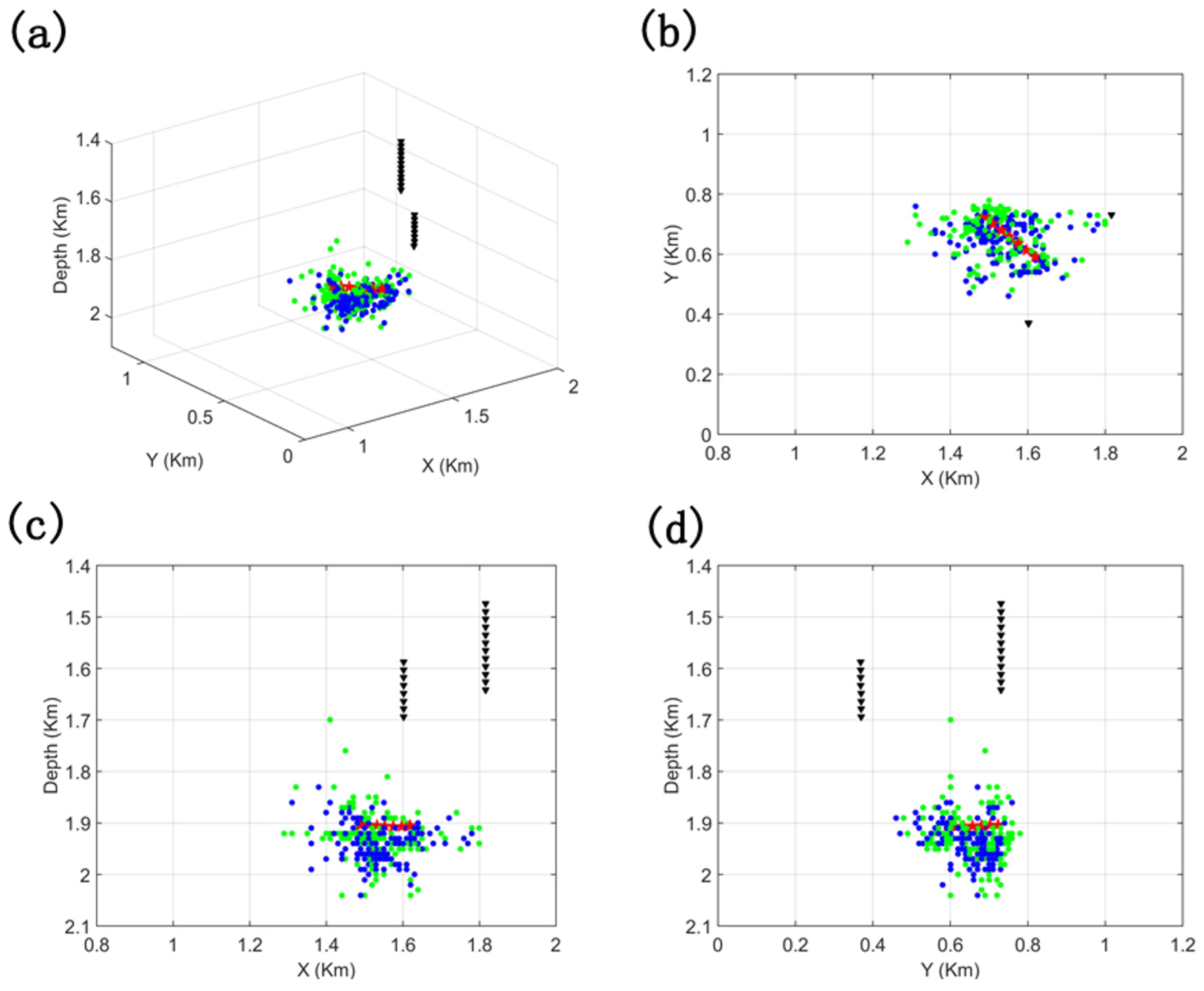
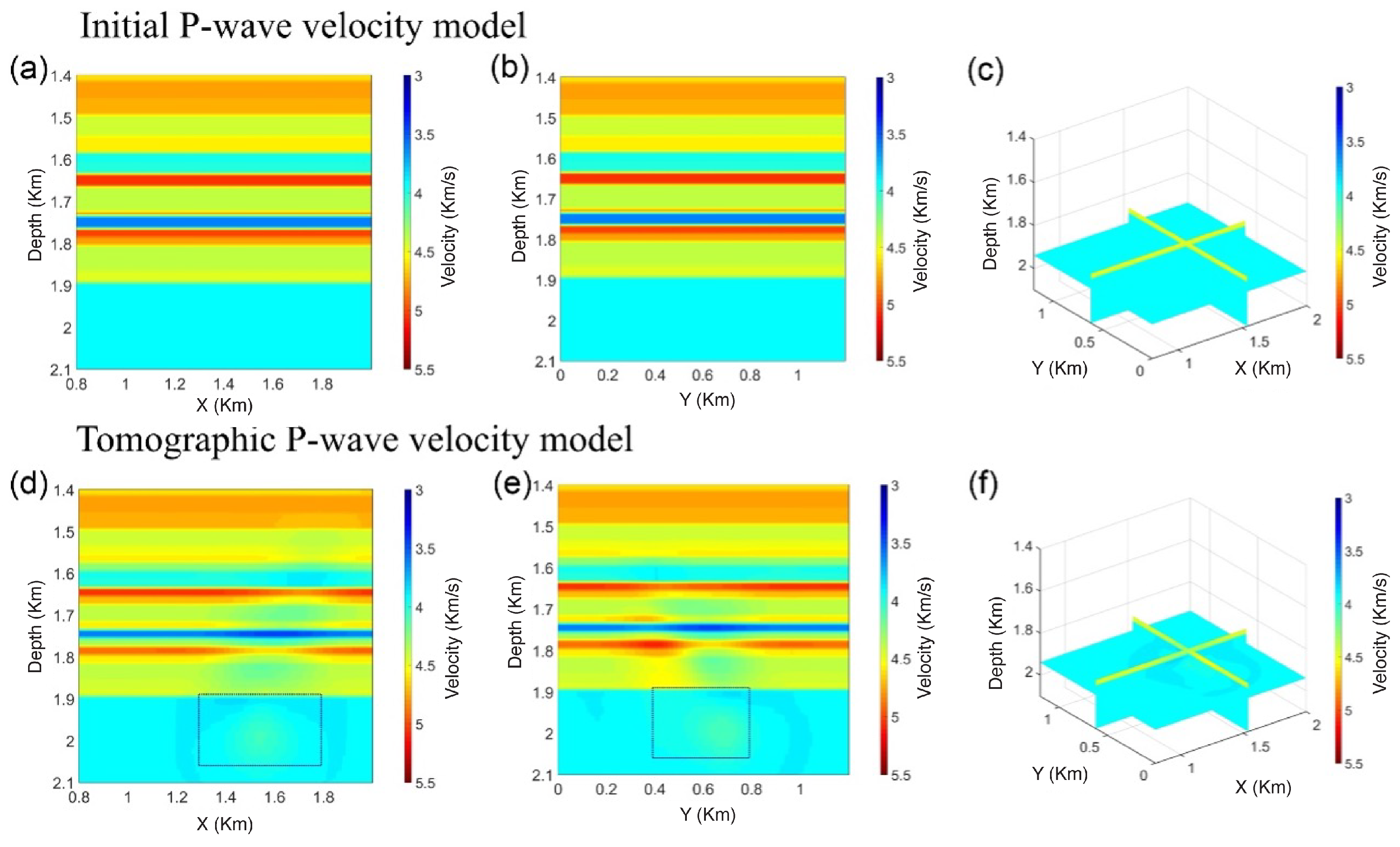
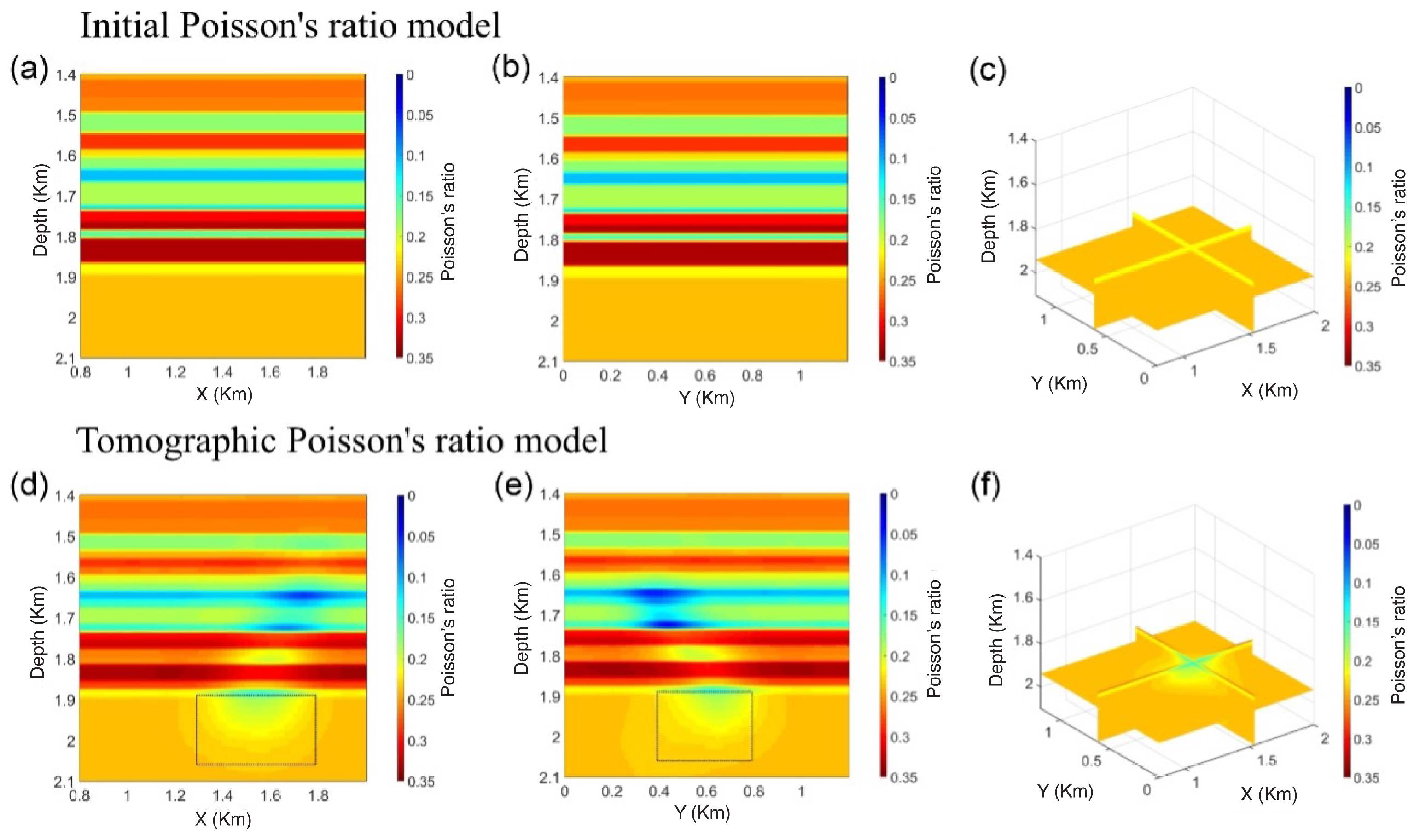
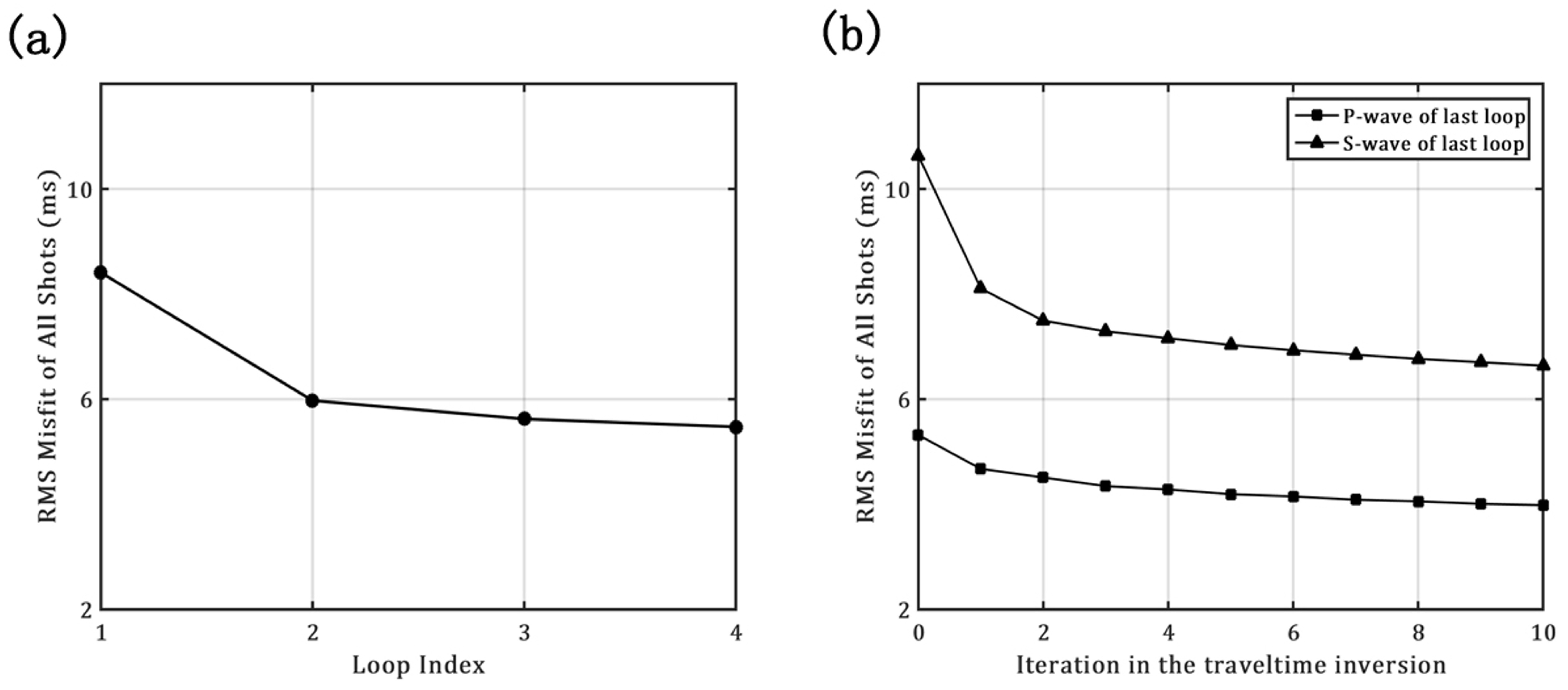
3.1. Synthetic Example

To evaluate the efficacy of our proposed method, we conduct a synthetic test featuring two observation wells and a simulated red cloud of 726 microseismic events as depicted in Figure 1. Each well is equipped with 20 receivers spaced 20 m apart. We design two-layered grid models for Vp and Vs, incorporating an abnormal volume within each layer, from which we derive the true Poisson’s ratio model. As illustrated in Figure 2a–c and Figure 3a–c, these anomalies represent the zones of hydraulic fracturing for a stimulation stage. We hypothesize that the red event cloud (shown in Figure 1) is triggered by fractures due to shear or tensile failure, which could increase porosity and permeability while significantly lowering the Poisson’s ratio. This stimulated region, or anomaly, is identified as the shale sweet spot. We initialize the models by altering the true Vp and Vs layered models by 5% and 10%, respectively, based on sonic logs or calibrated models. The initial Poisson’s ratio model is further obtained based on initial Vp and Vs models.

After establishing the velocity models and survey geometry, we employ 3D wavefront raytracing to compute the traveltime data based on the true event locations within the models. The synthetic data are treated as the observed or picked arrival times typically encountered in field situations. We iteratively invert the Vp and Poisson’s ratio and refine the event locations using the grid search method during each iteration loop. This process continues until the event locations stabilize and no longer change. As shown in Figure 1, the event locations determined by the grid search method closely match the true locations, with a maximum discrepancy of about 30 m. Notably, the error in the Y-axis positioning is less than that in the X-axis, which can be attributed to the constraints imposed by the two receiver arrays.

In addition to event localization, the final inversion results for the Vp and Poisson’s ratio models incorporate the initial models’ layer constraints. Figure 2 displays the Vp models—true, initial, and inverted—highlighting that the abnormal area (indicated by a black rectangle) near the event cloud is accurately recovered. Similarly, a comparison between the true and inverted Poisson’s ratio models in Figure 3 shows effective recovery of the abnormal area around the event cloud. These comparisons confirm that the embedded anomaly is well inverted, demonstrating the effectiveness of our methodology.

We also perform traditional traveltime tomography to invert Vp and Vs separately and subsequently derive Poisson’s ratio. We extract Vp and Poisson’s ratio profiles from both tomographic methods along two horizontal axes at a depth of 1.88 km. Figure 4 illustrates the comparison of the Vp and Poisson’s ratio images obtained from the traditional and our tomographic methods. The green lines represent the true models, while the blue and red lines depict results from our proposed and the traditional methods, respectively. The comparison reveals that the red lines, indicating our method, more accurately recover the abnormal area compared to the blue lines, demonstrating superior Vp and Poisson’s ratio solutions.

Throughout the procedure, we continuously monitor data misfit, which includes a 3D grid search for event location and simultaneous traveltime tomography for Vp and Poisson’s ratio models during each loop. Figure 5a displays the convergence curve of the data misfit across four loops. We limit the display to four loops, as subsequent loops do not further reduce the data misfit. Additionally, each traveltime tomography iteration involves ten iterations to achieve stable solutions. Figure 5b illustrates the traveltime misfit for each iteration in the final loop. In the traveltime tomography of each loop, we use the initial models rather than the inverted solutions from the previous loop. This approach helps to avoid biases that might arise from cumulative errors in the models during the tomography process.

3.2. Field Example

We further apply our method to a field case involving a microseismic dataset created during hydraulic fracturing in the Barnett Shale reservoir [43]. To ensure sufficient raypath coverage and high-quality data, we select 156 effective events recorded by two nearby vertical receiver arrays during the fifth stage of hydraulic stimulation. Figure 6 shows recordings from one event by both arrays, where P and S wave arrivals are clearly identifiable. One vertical well employs a recording system consisting of 12 three-component geophones, while the other uses 8. These geophones are spaced approximately 15 m apart. The deployment geometry of these geophones is illustrated in Figure 7.

We construct the initial Vp and Vs layer models from sonic logs, which provide velocity profiles along the wells, and convert these into 3D Vp and Vs grid models. From these grids, we calculate the Poisson’s ratio model. Using our proposed method, we continue refining the event locations and Vp and Poisson’s ratio models until the event locations stabilized. Figure 7a illustrates the 3D distribution of our event locations (blue dots) alongside those provided by a service company (green dots), showing an average discrepancy of about 30 m. We further project both sets of event results in different views (Figure 7b–d), observing that our event locations maintain a similar distribution to the green ones but with greater convergence. The seven red stars in Figure 7 mark the perforations during the fifth stage. From the X-Y plan view, our event locations correspond closely with these perforations, a result of the constraints imposed by two observation wells. The depth positioning from the X-Z and Y-Z plan views also aligns well with the service company’s data, reflecting the accuracy of our calibrated layer models.

Figure 8d–f and Figure 9d–f display the inversion results for Vp and Poisson’s ratio, respectively. Across various plan views, we identify a region with a relatively low Poisson’s ratio, marked by a black rectangle, located around a depth of 1.9 km. This low Poisson’s ratio area delineates the sweet spot and helps estimate the stimulated hydrocarbon volume. Figure 10 presents the data misfit curve, demonstrating the convergence of our method. Despite numerous iterations, the data misfit stabilizes after four loops as shown in Figure 10a. Additionally, we include the misfit curves for P- and S-wave traveltime tomography from the final loop, illustrating detailed convergence behavior.

4. Discussion

In our synthetic examples, we demonstrate the capability of using two observation wells to effectively map the sweet spot, characterized by a low Poisson’s ratio distribution. Both the event locations and velocity solutions are accurately recovered. However, as the distance between events and receivers increases, the effectiveness of recovering event locations and structural models decreases. Furthermore, using just one monitoring well proves insufficient for effectively recovering event locations and velocities. By testing our method with three observation wells arranged in a triangular distribution, we significantly improve the accuracy of both event locations and velocity results. These tests highlight the importance of sufficient ray coverage to balance the trade-off between event locations and structural models. Our findings suggest that with at least two strategically positioned observation wells, our method can effectively reconstruct Vp and Poisson’s ratio models.

Our method uses 3D grid search to locate events without requiring prior known locations. Initial velocity models are directly constructed from sonic logs. With high-quality observed data and well-prepared initial models, we successfully derive reliable Poisson’s ratio models and map sweet spots. In complex geological settings, the disparity between P and S rays might lead to biased Poisson’s ratio results from the conventional Vp and Vs models [44]. Traditional techniques, such as calculating the Vp/Vs ratio [45] or inverting S-P time ratios [14,22], might inaccurately estimate Poisson’s ratio or Vp/Vs models under such conditions. Our method, not assuming identical P- and S-wave raypaths, avoids biases from unresolved portions of the Vp model. In synthetic tests, our traveltime tomography produces more accurate P-wave velocity and Poisson’s ratio solutions than traditional methods. However, in real cases where P- and S-wave raypaths are similar due to the short distances between events and receivers, our method does not show significant improvements over traditional techniques.

We observe that the cluster of induced events correlates strongly with the low Poisson’s ratio area marked by a black rectangle in Figure 9. This anomaly in Poisson’s ratio could indicate changes in the shale rock properties triggered by high-pressure fluid injection during fracturing. The treatment enhances porosity and permeability, allowing hydrocarbons to fill the fractures and subsequently lower the Poisson’s ratio. Thus, a low Poisson’s ratio can serve as an indicator for predicting hydrocarbon presence or sweet spots. In our field example, the limited data restrict our analysis to only one stimulation stage, impacting the resolution and accuracy of the sweet spot map. However, with more data, we could produce a more precise and detailed map, which would aid in estimating the volume of the reservoir stimulated during hydraulic fracturing, applicable to widespread unconventional hydrocarbon [46] and geothermal [47] exploitations.

5. Conclusions

In this study, we introduce an alternating method that integrates 3D traveltime tomography with 3D grid search to recover 3D Vp, Poisson’s ratio models, and event locations. Our synthetic tests validate the capability of this method to directly reconstruct 3D Vp and Poisson’s ratio models within the event area, achieving the accurate identification of the low Poisson’s ratio areas, which we associate with sweet spots. Field examples further demonstrate the method’s effectiveness, yielding reliable event locations and promising Poisson’s ratio models. These locations help characterize fractures, and the anomalies identified in low Poisson ratios can estimate the volume of stimulated reservoirs. With adequate ray coverage, our method can accurately map Poisson ratio distributions, helping to identify sweet spots in shale reservoirs.

References

1. Schenk, C.J. Geologic definition of conventional and continuous accumulations in select US basins—The 2001 approach. In Proceedings of the Abstract for AAPG Hedberg Research Conference on Understanding, Exploring and Developing Tight Gas Sands, Vail, CO, USA, 24–29 April 2005. [Google Scholar]
2. Norton, M.; Hovdebo, W.; Cho, D.; Maxwell, S.; Jones, M. Integration of surface seismic and microseismic for the characterization of a shale gas reservoir. CSEG Rec. 2011, 34, 31–33. [Google Scholar]
3. Holbrook, W.S.; Gajewski, D.; Krammer, A.; Prodehl, C. An interpretation of wide-angle compressional and shear wave data in southwest Germany: Poisson’s ratio and petrological implications. J. Geophys. Res. Solid Earth 1988, 93, 12081–12106. [Google Scholar] [CrossRef]
4. Ikwuakor, K.C. The Vp/Vs ratio after 40 years: Uses and abuses. In Proceedings of the SEG International Exposition and Annual Meeting, SEG–2006, New Orleans, LA, USA, 1–6 October 2006. [Google Scholar]
5. McCormack, M.; Justice, M.; Sharp, W. A Stratigraphic Interpretation of Shear and Compressional Wave Seismic Data for the Pennsylvanian Morrow Formation of Southeastern New Mexico: Chapter 13. AAPG Spec. Vol. 1985, 225–239. [Google Scholar]
6. Tatham, R.H. V p/V s and lithology. Geophysics 1982, 47, 336–344. [Google Scholar] [CrossRef]
7. Anderson, P.F. A Comparison of Inversion Techniques for Estimating Vp/Vs from 3-C 3-D Seismic Data. Proc. Masters Abstr. Int. 2010, 49, 3. [Google Scholar]
8. Goodway, B.; Chen, T.; Downton, J. Improved AVO fluid detection and lithology discrimination using Lamé petrophysical parameters;“λρ”,“μρ”, & “λ/μ fluid stack”, from P and S inversions. In SEG Technical Program Expanded Abstracts 1997; Society of Exploration Geophysicists: Houston, TX, USA, 1997; pp. 183–186. [Google Scholar]
9. Hampson, D.P.; Russell, B.H.; Bankhead, B. Simultaneous inversion of pre-stack seismic data. In SEG Technical Program Expanded Abstracts 2005; Society of Exploration Geophysicists: Houston, TX, USA, 2005; pp. 1633–1637. [Google Scholar]
10. Martakis, N.; Tselentis, A.; Kapotas, S.; Karageorgi, E. Passive Seismic Tomography a Complementary Geophysical Method–Successful Case Study. In Proceedings of the 65th EAGE Conference & Exhibition, European Association of Geoscientists & Engineers, Stavanger, Norway, 2–5 June 2003; p. cp-6-00074. [Google Scholar]
11. Martakis, N.; Kapotas, S.; Tselentis, G. Integrated passive seismic acquisition and methodology. Case Studies. Geophys. Prospect. 2006, 54, 829–847. [Google Scholar] [CrossRef]
12. Thurber, C.H.; Atre, S.R.; Eberhart-Phillips, D. Three-dimensional Vp and Vp/Vs structure at Loma Prieta, California, from local earthquake tomography. Geophys. Res. Lett. 1995, 22, 3079–3082. [Google Scholar] [CrossRef]
13. Eberhart-Phillips, D.; Michael, A.J. Seismotectonics of the Loma Prieta, California, region determined from three-dimensional V p, V p/V s, and seismicity. J. Geophys. Res. Solid Earth 1998, 103, 21099–21120. [Google Scholar] [CrossRef]
14. Chiarabba, C.; Amato, A. Vp and Vp/Vs images in the Mw 6.0 Colfiorito fault region (central Italy): A contribution to the understanding of seismotectonic and seismogenic processes. J. Geophys. Res. Solid Earth 2003, 108, B5. [Google Scholar] [CrossRef]
15. Thurber, C.H. Analysis methods for kinematic data from local earthquakes. Rev. Geophys. 1986, 24, 793–805. [Google Scholar] [CrossRef]
16. Kissling, E. Geotomography with local earthquake data. Rev. Geophys. 1988, 26, 659–698. [Google Scholar] [CrossRef]
17. Iyer, H.; Hirahara, K. Seismic Tomography: Theory and Practice; Springer Science & Business Media: Berlin, Germany, 1993. [Google Scholar]
18. Rutledge, J.T.; Phillips, W.S. Hydraulic stimulation of natural fractures as revealed by induced microearthquakes, Carthage Cotton Valley gas field, east Texas. Geophysics 2003, 68, 441–452. [Google Scholar] [CrossRef]
19. Maxwell, S.C.; Urbancic, T.I. The role of passive microseismic monitoring in the instrumented oil field. Lead. Edge 2001, 20, 636–639. [Google Scholar] [CrossRef]
20. Treadgold, G.; Campbell, B.; McLain, B.; Sinclair, S.; Nicklin, D. Eagle Ford shale prospecting with 3D seismic data within a tectonic and depositional system framework. The Leading Edge 2011, 30, 48–53. [Google Scholar] [CrossRef]
21. Valoroso, L.; Improta, L.; De Gori, P.; Di Stefano, R.; Chiaraluce, L. From 3D to 4D Passive Seismic Tomography-The Sub-surface Structure Imaging of the Val d’Agri Region, Southern Italy. In Proceedings of the 70th EAGE Conference and Exhibition incorporating SPE EUROPEC 2008, European Association of Geoscientists & Engineers, Rome, Italy, 9–12 June 2008; p. cp-40-00309. [Google Scholar]
22. Zhang, H.; Thurber, C.; Bedrosian, P. Joint inversion for vp, vs, and vp/vs at SAFOD, Parkfield, California. Geochem. Geophys. Geosyst. 2009, 10. [Google Scholar] [CrossRef]
23. Tselentis, G.A.; Martakis, N.; Paraskevopoulos, P.; Lois, A. High-resolution passive seismic tomography for 3D velocity, Poisson’s ratio ν, and P-wave quality QP in the Delvina hydrocarbon field, southern Albania. Geophysics 2011, 76, B89–B112. [Google Scholar] [CrossRef]
24. Barthwal, H.; van der Baan, M. Passive seismic tomography using recorded microseismicity. In Proceedings of the SEG International Exposition and Annual Meeting, SEG–2014, Denver, CO, USA, 26–31 October 2014. [Google Scholar]
25. Chatterjee, S.; Pitt, A.; Iyer, H. Vp/Vs ratios in the Yellowstone national park region, Wyoming. J. Volcanol. Geotherm. Res. 1985, 26, 213–230. [Google Scholar] [CrossRef]
26. Julian, B.; Ross, A.; Foulger, G.; Evans, J. Three-dimensional seismic image of a geothermal reservoir: The Geysers, California. Geophys. Res. Lett. 1996, 23, 685–688. [Google Scholar] [CrossRef]
27. Lees, J.M.; Wu, H. Poisson’s ratio and porosity at Coso geothermal area, California. J. Volcanol. Geotherm. Res. 2000, 95, 157–173. [Google Scholar] [CrossRef]
28. Lees, J.M. Three-dimensional anatomy of a geothermal field, Coso, southeast-central California. Geol. Soc. Am. Mem. 2002, 195, 259–276. [Google Scholar]
29. Hauksson, E.; Unruh, J. Regional tectonics of the Coso geothermal area along the intracontinental plate boundary in central eastern California: Three-dimensional Vp and Vp/Vs models, spatial-temporal seismicity patterns, and seismogenic deformation. J. Geophys. Res. Solid Earth 2007, 112, B6. [Google Scholar] [CrossRef]
30. Kummerow, J.; Reshetnikov, A.; Hring, M.; Asanuma, H. Distribution of the Vp/Vs ratio within the Basel 1 geothermal reservoir from microseismic data. In Proceedings of the 74th EAGE Conference and Exhibition incorporating EUROPEC 2012, European Association of Geoscientists & Engineers, Copenhagen, Denmark, 4–7 June 2012; p. cp-293-00092. [Google Scholar]
31. Zang, A.; Oye, V.; Jousset, P.; Deichmann, N.; Gritto, R.; McGarr, A.; Majer, E.; Bruhn, D. Analysis of induced seismicity in geothermal reservoirs—An overview. Geothermics 2014, 52, 6–21. [Google Scholar] [CrossRef]
32. Maxwell, S. Microseismic location uncertainty. CSEG Rec. 2009, 34, 41–46. [Google Scholar]
33. Thurber, C.H. Hypocenter-velocity structure coupling in local earthquake tomography. Phys. Earth Planet. Inter. 1992, 75, 55–62. [Google Scholar] [CrossRef]
34. Thurber, C.; Eberhart-Phillips, D. Local earthquake tomography with flexible gridding. Comput. Geosci. 1999, 25, 809–818. [Google Scholar] [CrossRef]
35. Concha, D.; Fehler, M.; Zhang, H.; Wang, P. Imaging of the Soultz enhanced geothermal reservoir using microseismic data. In Proceedings of the Thirty-Fifth Workshop on Geothermal Reservoir Engineering Stanford University, Stanford, CA, USA, 1–3 February 2010. [Google Scholar]
36. Jansky, J.; Plicka, V.; Eisner, L. Feasibility of joint 1D velocity model and event location inversion by the neighbourhood algorithm. Geophys. Prospect. 2010, 58, 229–234. [Google Scholar] [CrossRef]
37. Zhou, R.; Huang, L.; Rutledge, J. Microseismic event location for monitoring CO2 injection using double-difference tomography. Lead. Edge 2010, 29, 208–214. [Google Scholar] [CrossRef]
38. Rodi, W.; Toksöz, M.N. Grid-search techniques for seismic event location. In Proceedings of the 22nd Annual DoD/DOE Seismic Research Symposium: Planning for Verification of and Compliance with the Comprehensive Nuclear-Test-Ban Treaty, Defense Threat Reduction Agency, Dulles, Virginia, 1 August 2000. [Google Scholar]
39. Eberhart-Phillips, D. Three-dimensional P and S velocity structure in the Coalinga region, California. J. Geophys. Res. Solid Earth 1990, 95, 15343–15363. [Google Scholar] [CrossRef]
40. Aldridge, D.F.; Bartel, L.C.; Symons, N.P.; Warpinski, N.R. Grid search algorithm for 3D seismic source location. In Proceedings of the SEG International Exposition and Annual Meeting, SEG–2003, Dallas, TX, USA, 26–31 October 2003. [Google Scholar]
41. Sethian, J.A.; Popovici, A.M. 3-D traveltime computation using the fast marching method. Geophysics 1999, 64, 516–523. [Google Scholar] [CrossRef]
42. Nolet, G. Waveform tomography. In Seismic Tomography: With Applications in Global Seismology and Exploration Geophysics; Springer: Berlin, Germany, 1987; pp. 301–322. [Google Scholar]
43. Kuang, W.; Zoback, M.; Zhang, J. Estimating geomechanical parameters from microseismic plane focal mechanisms recorded during multistage hydraulic fracturing. Geophysics 2017, 82, KS1–KS11. [Google Scholar] [CrossRef]
44. Nicholson, C.; Simpson, D.W. Changes in Vp/Vs with depth: Implications for appropriate velocity models, improved earthquake locations, and material properties of the upper crust. Bull. Seismol. Soc. Am. 1985, 75, 1105–1123. [Google Scholar]
45. Nakamura, M.; Yoshida, Y.; Zhao, D.; Katao, H.; Nishimura, S. Three-dimensional P-and S-wave velocity structures beneath the Ryukyu arc. Tectonophysics 2003, 369, 121–143. [Google Scholar] [CrossRef]
46. Kokkinos, N.; Nkagbu, D.; Marmanis, D.; Dermentzis, K.; Maliaris, G. Evolution of Unconventional Hydrocarbons: Past, Present, Future and Environmental FootPrint. J. Eng. Sci. Technol. Rev. 2022, 15, 15–24. [Google Scholar] [CrossRef]
47. Sharmin, T.; Khan, N.R.; Akram, M.S.; Ehsan, M.M. A state-of-the-art review on geothermal energy extraction, utilization, and improvement strategies: Conventional, hybridized, and enhanced geothermal systems. Int. J. Thermofluids 2023, 18, 100323. [Google Scholar] [CrossRef]
Figure 1. The survey geometry and event location results in the synthetic case. The black reverse triangles denote two receiver arrays installed in two wells. The red and blue dots are the true and searched event locations, respectively. (a) 3D view; (b) X-Y plan view; (c) X-Z plan view; and (d) Y-Z plan view.
Applsci 14 08056 g001
Figure 2. True, initial, and inverted P-wave velocity models in the synthetic case. (a,d,g) Plan view (Y = 1.0 Km), (b,e,h) plan view (X = 0.86 Km), and (c,f,i) cross-sectional view (X = 0.86 Km, Y = 1.0 Km, and Z = 1.9 Km). (ac) Map views of true 3D P-wave velocity model. (df) Map views of initial 3D P-wave velocity model. (gi) Map views of the inverted 3D P-wave velocity result. The black rectangle denotes the border of the embedded anomaly in the true model.
Applsci 14 08056 g002
Figure 3. True, initial, and inverted Poisson’s ratio models in the synthetic case. (a,d,g) Plan view (Y = 1.0 Km), (b,e,h) plan view (X = 0.86 Km), and (c,f,i) cross-sectional view (X = 0.86 Km, Y = 1.0 Km, and Z = 1.9 Km). (ac) Map views of true 3D Poisson’s ratio model. (df) Map views of initial 3D Poisson’s ratio model. (gi) Map views of the inverted 3D Poisson’s ratio result. The black rectangle denotes the border of the embedded anomaly in the true model.
Applsci 14 08056 g003
Figure 4. The Vp (a) and Poisson’s ratio (b) images extracted along two horizontal directions at a depth of 1.88 km of tomographic models. The green and red lines represent the images of true and inverted Vp or Poisson’s ratio models with our traveltime tomographic methods, the blue lines are the images of the Vp and derived Poisson’s ratio models from Vp and Vs models inverted separately using standard traveltime tomography.
Applsci 14 08056 g004
Figure 5. (a) Convergence curve of location error of 3D grid search over three loops in the synthetic case. (b) Misfit curves of the traveltime tomography of the last loop. The circle represents the data misfit of each loop, and the triangles and squares are the traveltime misfits over each iteration of P and S waves, respectively.
Applsci 14 08056 g005
Figure 6. The different recordings of the same microseismic event from (a) eight-receiver array and (b) twelve-receiver array, respectively, in one field case. The P- and S-wave arrivals display a high signal-to-noise ratio and are easily picked (red and blue, respectively) on all 20 receivers.
Applsci 14 08056 g006
Figure 7. The survey geometry and event location results of the field case. The black reverse triangles stand for two receiver arrays installed in the two monitoring wells. The seven red stars are the perforations in one stage. The blue dots are our searched location results, and the green dots are the location results provided by service company. (a) The 3D view; (b) X-Y plan view; (c) X-Z plan view; and (d) Y-Z plan view.
Applsci 14 08056 g007
Figure 8. Initial and inverted P-wave velocity models in the field case. (a,d) Plan view (Y = 1.0 Km), (b,e) plan view (X = 0.86 Km), and (c,f) cross-sectional view (X = 0.86 Km, Y = 1.0 Km, and Z = 1.9 Km). (ac) Map views of initial 3D P-wave velocity model. (df) Map views of the inverted 3D P-wave velocity result.
Applsci 14 08056 g008
Figure 9. Initial and inverted Poisson’s ratio models in the field case. (a,d) Plan view (Y = 1.0 Km), (b,e) plan view (X = 0.86 Km), and (c,f) cross-sectional view (X = 0.86 Km, Y = 1.0 Km, and Z = 1.9 Km). (ac) Map views of initial 3D Poisson’s ratio model. (df) Map views of the inverted 3D Poisson’s ratio result.
Applsci 14 08056 g009
Figure 10. (a) Convergence curve of location error of 3D grid search over three loops in the field case. (b) Misfit curves of the traveltime tomography of the last loop. The circle represents the data misfit of each loop, and the triangle and square are the traveltime misfits over each iteration of P and S waves, respectively.
Applsci 14 08056 g010
Disclaimer/Publisher’s Note: The statements, opinions and data contained in all publications are solely those of the individual author(s) and contributor(s) and not of MDPI and/or the editor(s). MDPI and/or the editor(s) disclaim responsibility for any injury to people or property resulting from any ideas, methods, instructions or products referred to in the content.