Levitating Control System of Maglev Ruler Based on Active Disturbance Rejection Controller

Abstract

The autonomous displacement and displacement measurement functions of the maglev ruler are performed by the mover core. The magnetic levitation ruler can serve as a viable alternative to the linear measurement system of a coordinate measuring machine. The stability of the four magnetic fields in air gaps and the levitation position of the maglev ruler is one of the key factors for the stability of the thrust force on the power core, and it is also one of the key factors for ensuring the precision of the maglev ruler. There is cross-coupling between the two ends of the mover core of the maglev ruler, resulting in a strongly coupled, nonlinear, multi-input and multi-output system for the levitating system of the maglev ruler. This paper establishes a mathematical model for the levitating system of the maglev ruler and designs a levitating control system for the maglev ruler based on an active disturbance rejection control algorithm to achieve decoupling and disturbance suppression. Through simulation analysis and experimental testing of the levitating system with starting and disturbance, it is proved that the levitating control system of the maglev ruler has good dynamic characteristics, static characteristics, and robustness.

1. Introduction

A coordinate measuring machine (CMM) is capable of measuring free-form surface components, and its linear measurement system comprises a grating scale, servo motor, and linear motion mechanism. The magnetic levitation ruler can streamline the linear measurement system of the CMM. The two functions of the maglev ruler (MR), autonomous displacement and displacement measurement, are completed by its mover core (MC) [1]. This MC adopts a step-by-step autonomous displacement. Each step length is the scale of the MR. While performing autonomous displacement, the displacement is converted into a pulse quantity, which is sent to the microcontroller to complete displacement measurement. Obviously, the stability of the step length improves the precision of the maglev rule. According to Newton’s second law of motion, the stability of the thrust force applied to the MC determines the stability of the step length. The stability of the magnetic field in air gaps and the current of the horizontal control coil determine the stability of the thrust force [1,2]. The four air-gap magnetic fields of the MR exhibit coupling and are susceptible to external interference, being regulated by four levitating control coils. Additionally, these magnetic fields play a pivotal role in determining the levitating height of the MC. Consequently, the levitating control system of the MR can be characterized as a coupled four-input, two-output system [1]. This paper mainly studies how to improve the stability of the magnetic field in air gaps through the levitating control system of the MR.

The maglev ball system can be used as an experimental device to verify the maglev control method. Its working principle is to generate magnetic force through electromagnets to balance the gravity of the ball. Therefore, the ball is stably levitated at the equilibrium point. The coil current of the electromagnet determines the levitating position of the ball [3]. Victor [4] et al. discussed the role of direct-current to direct-current (DC/DC) converters in magnetic suspension systems and verified the feasibility of a magnetic suspension positioning system that included a proportional, integral, differential (PID) algorithm for a maglev ball as the research object. Debdoot Sain [5] proposed a maglev positioning system based on a 2-DOF PID controller, which was used for the positioning of maglev balls [5]. Aysen [6] et al. proposed an opposing artificial electric field algorithm (OBAEFA), which was used in the adjustment of fractional order PID (FOPID) control systems [6]. FOPID was used in the maglev ball positioning system [6]. The OBAEFA is an upgraded version of the artificial electric field algorithm (AEFA), using an opposing learning strategy to enhance the search capabilities of the AEFA algorithm [6]. The experimental results verified the superiority of OBAEFA [6]. In the maglev ball positioning system, the OBAEFA was used to debug FOPID, which optimized the transient response of the positioning system by minimizing an optimization objective function with a simple structure [7]. T. Deepa [8] compared and analyzed the control performance of PID controller and linear quadratic regulator (LQR) controller [8]. It proved that the use of LQR controllers improved the performance of maglev systems [8]. S. Pandey [9,10,11] studied how to apply the fractional-order sliding mode controllers in maglev ball positioning systems [9,10,11]. Rahul Sanmugam Gopi et al. [12] proposed a new adaptive control method for ball position controllers to improve maglev systems. The method included proportional integral speed plus feedforward in the control structure and used a modified version of the standard tuning rule as the adaptive mechanism [12]. The control method was applied to the maglev ball positioning system. Kim S. K. et al. [13] studied a sensorless nonlinear controller for maglev ball positioning systems [13]. Massive studies have revealed the characteristics of the magnetic field in the air gap of the maglev ball and the control method for the levitating position of the maglev ball, providing a reference for the study of the levitating system of the MC of the MR in this paper. However, the maglev ball only has one air gap. The levitating control method of the maglev ball cannot be applied to the MR.

Zhou Zhenxiong et al. [14] studied the levitating system of the TU-type maglev platform [14]. The four basic levitation magnetic loops of the TU-type maglev platform are the same as those of the MR [14]. The T-shaped mover of the TU-type maglev platform has three ends [14]. There are two air gaps between each end and the stator yoke, an upper air gap and a lower air gap [14]. The magnetic flux in the upper and lower air gaps determines the force on the ends where they are located, controlling the levitation height of the ends [14]. The magnetic flux in the air gap can also be divided into two parts, one from the permanent magnet and the other from the levitating control coil [14]. The magnetic flux emitted by the levitating control coil is related to the current of the levitating control coil [14]. Therefore, the magnetic flux emitted by the levitating coil can adjust the size of the air gap flux, thus achieving stable levitation of the T-shaped mover [14]. However, the TU-type maglev platform uses one coil to control the upper and lower air gap fluxes at one end, which cannot solve the simultaneous asynchronous interference in the two air gap fluxes [14]. In addition, due to the use of one control coil to adjust the magnetic flux in the upper and lower air gaps, there is a commutation problem in the current of the control coil [14]. The control coil is an inductance and an energy storage element [14]. During current commutation, there is a transition process, causing the current in the control coil to have a turning point at the commutation point [14]. Therefore, the TU-type maglev platform is equipped with only two levitating control magnetic circuits, making it incapable of independently regulating four air gaps. Furthermore, the current flowing through the levitating control coil of the TU-type maglev platform does not exhibit a linear relationship with time. The MR establishes four levitating control magnetic loops. The magnetic flux of each magnetic loop can be independently controlled, eliminating the need for current commutation of the levitating coil, eliminating the inflection point, and allowing independent control of the magnetic flux in each air gap. The working principle of the levitating system of the MR is analyzed, and a mathematical model of the levitating system is established in this paper. The levitating system uses an active disturbance rejection control (ADRC) control algorithm to stabilize the levitation position of the MC while also stabilizing the magnetic field in air gaps.

The structure of this paper is as follows: In the second part, this paper analyzes the characteristics of the maglev system of the MR and establishes a mathematical model. In the third part, this paper designs a maglev control system based on ADRC according to the characteristics of the maglev system of the MR and conducts simulation analysis on the maglev control system. In every fourth part, this paper conducts experimental testing on the maglev control system. The organization of this paper is as follows. In Section 2, the characteristics of the maglev system of the MR are analyzed, and a mathematical model is established. In Section 3, according to the characteristics of the maglev system, a levitating control system based on ADRC was designed, and a simulation analysis of the levitating control system was conducted. In Section 4, an experimental test was conducted on the levitating control system. Finally, conclusions are presented in Section 5.

2. Analysis Model of Levitating Force

Changes in the horizontal position of the mover core result in variations in the length of the magnetic circuit, subsequently altering the air gap magnetic field and ultimately affecting the levitating force [1]. Evidently, there exists a correlation between the levitating force and the planar position of the mover core. Given the intricate coupling among the levitating heights at both ends of the mover core and its planar position [1], a simplistic modeling approach that treats these three parts as mutually independent systems fails to capture the intricate working principle of internal coupling within the system. Consequently, such a model diverges significantly from the actual object, rendering it challenging to achieve high-performance control.

This article establishes a relatively precise mathematical model by conducting a thorough analysis of the magnetic circuit and forces involved in the MR. This model effectively uncovers the intricate coupling relationships between the levitating heights at both ends of the mover core, as well as the intricate coupling between the levitating height and the plane position. Notably, this model is well suited for the application of the ADRC control method.

2.1. Magnetic Potential Calculation and Leakage Coefficient

The MR uses four permanent magnets to provide bias magnetic fields for the six air gaps of the system. The magnetic field strength of the four permanent magnets was analyzed using finite element analysis, and their average values were:

Average magnetic field intensity: H_BM = 265 × 10³ A/m.

The average magnetic potential of permanent magnets: V_m = H_BM ∙ l_BM = 2650 A.

The MR system chooses four permanent magnets of the same size, so the magnetic field strength of the four permanent magnets can also be considered to be the same.

There are two types of magnetic levitating loops: the first is a basic levitating loop based on permanent magnets, which produces bias magnetic fields in the air gap; the second is a control levitating loop based on levitating coils, which produces control magnetic fluxes. During the operation of the MR, its MC is in a magnetic saturation state. Therefore, there must be significant magnetic losses and magnetic leakage in the magnetic loop, and two types of leakage coefficients need to be introduced to compensate for the air gap reluctance model.

The two magnetic leakage coefficients are:

σ_BM is the leakage factor of the basic levitating loop;

σ_CM is the leakage factor of the control levitating loop.

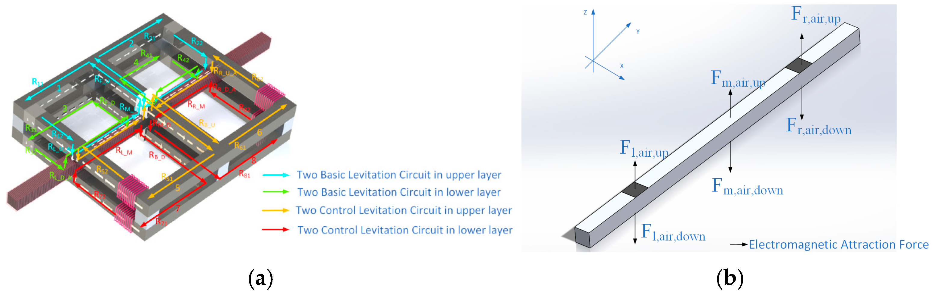
2.2. Analysis Model of Buoyancy Force

The levitating force of the MC comes from three parts: the electromagnetic suction force on the left support, the right support, and the center point. The schematic diagram of the electromagnetic suction force on the magnetic loop and the MC is shown in Figure 1.

The MR is divided into three parts, the left, right, and middle, as shown in Figure 1b. The levitating force in the middle is affected by the levitating forces on the left and right, and these levitating forces are similar. Therefore, this paper first studies the levitating force using the left levitating force as an example.

Figure 1b also indicates the electromagnetic suction force acting on the MC. The resultant force of the upper and lower electromagnetic suction forces on the MC is the left levitating force:

$$F_{left}=F_{l\_air\_up}-F_{l\_air\_down}$$

(1)

where F_left is the levitating force on the left end of MC, F_{l_air_up} is the upward electromagnetic suction force on the left end of MC, and F_{l_air_down} is the downward electromagnetic suction force on the left end of MC.

According to the electromagnetic suction force calculation equation [15]:

$$F_R=-{\displaystyle \frac{1}{2}}{\displaystyle \frac{{\varphi }^2}{{\mu }_0\cdot A}}$$

(2)

where μ₀ is the permeability of the air gap; A is the area of the pole surface, which is the vertical intersection of the U-shaped conductor and the MC, i.e., the black area on the MC in Figure 1b. Therefore, the electromagnetic suction force F_R is proportional to the square of the magnetic flux $\varphi$ [1].

There are eight magnetic loops on the MR, which are numbered as shown in Figure 1a. The magnetic fluxes of the loop 1 to loop 8 magnetic loops are respectively: $\varphi$1, $\varphi$2, $\varphi$3, $\varphi$4, $\varphi$5, $\varphi$6, $\varphi$7, and $\varphi$8. Among them, $\varphi$1, $\varphi$2, $\varphi$3, and $\varphi$4 are the magnetic fluxes of the basic levitating loop; $\varphi$5, $\varphi$6, $\varphi$7, and $\varphi$8 are the magnetic fluxes of the control levitating loop.

As shown in Figure 1a, the magnetic flux in the upper air gap on the left support is the sum of the magnetic flux of the base levitating loop and the control levitating loop, and both directions are downward. Therefore, the calculation equation for the magnetic flux in the upper air gap on the left support is [16]:

$${\varphi }_{l\_up\_air}={\varphi }_1+{\varphi }_5$$

(3)

Similarly, the magnetic flux in the lower air gap of the left support is also the sum of the magnetic flux of the base levitating loop and the control levitating loop, and both directions are upward. Therefore, the calculation equation for the magnetic flux in the lower air gap of the left support is [16]:

$${\varphi }_{l\_down\_air}={\varphi }_3+{\varphi }_7$$

(4)

The total magnetic flux of the air gap in the upper part of the left support starts from the left upper permanent magnet and the left upper levitating coil. According to Hopkinson’s law [16]:

$$\varphi ={\displaystyle \frac{V}{R}}$$

(5)

where V represents the magnetic potential and R represents the magnetic reluctance.

As can be seen from Figure 1, the structures of the eight levitation magnetic loops are similar, consisting of permanent magnets or levitating coils and six magnetic conductors. For ease of calculation, a label is assigned to the magnetic reluctance of each magnetic conductor, as shown in Figure 1a.

As shown in Figure 1a, the MR has 28 magnetic resistors, including R₁₁, R₁₂, R₂₁, R₂₂, R₃₁, R₃₂, R₄₁, R₄₂, R₅₁, R₅₂, R₆₁, R₆₂, R₇₁, R₇₂, R₈₁, R₈₂, R_{M_U}, R_{M_D}, R_{F_U}, R_{F_D}, R_{B_U}, R_{B_D}, R_{L_M}, R_{R_M}, R_{L_U_A}, R_{L_D_A}, R_{R_U_A}, R_{R_D_A}. The air gap length of the MR can also be divided into two parts: the nominal air gap length and the coil air gap length occupied by the coil. In addition, due to the different leakage coefficients of the basic levitating loop and the control levitating loop, R_{M_U}, R_{M_D}, R_{L_U_A}, R_{L_D_A}, R_{R_U_A}, R_{R_D_A} can also be decomposed into R_{M_U_B}, R_{M_U_C}, R_{M_D_B}, R_{M_D_C}, R_{L_U_A_B}, R_{L_U_A_C}, R_{LCU_U}, R_{L_D_A_B}, R_{L_D_A_C}, R_{LCU_D}.

The known equation for calculating the magnetic reluctance is as follows [17]:

$$R={\displaystyle \frac{l}{\mu A}}$$

(6)

According to the dimensions of the components of the MR [1], combined with the magnetic reluctance calculation Equation (6) and the finite element analysis results, the following magnetic reluctance calculation equations can be obtained:

$$R_{11}=R_{21}=R_{31}=R_{41}={\displaystyle \frac{l_h}{{\mu }_{h\_f}A}}$$

(7)

$$R_{51}=R_{61}=R_{71}=R_{81}={\displaystyle \frac{l_h}{{\mu }_{h\_b}A}}$$

(8)

$$R_{L\_M}=R_{R\_M}={\displaystyle \frac{l_h}{{\mu }_{h\_m}A}}$$

(9)

$$R_{12}=R_{22}=R_{32}=R_{42}={\displaystyle \frac{l_{s\_y0}-y}{{\mu }_{b\_s}A}}$$

(10)

$$R_{52}=R_{62}=R_{72}=R_{82}={\displaystyle \frac{l_{s\_y0}+y}{{\mu }_{c\_s}A}}$$

(11)

$$R_{F\_D}=R_{F\_U}={\displaystyle \frac{l_{m\_y0}-y}{{\mu }_{f\_m}A}}$$

(12)

$$R_{B\_D}=R_{B\_U}={\displaystyle \frac{l_{m\_y0}+y}{{\mu }_{b\_m}A}}$$

(13)

$$R_{L\_U\_A\_B}={\displaystyle \frac{(l_A-z_l)}{{\mu }_{air}A{\sigma }_{BM}}}$$

(14)

$$R_{L\_D\_A\_B}={\displaystyle \frac{(l_A+z_l)}{{\mu }_{air}A{\sigma }_{BM}}}$$

(15)

$$R_{R\_U\_A\_B}={\displaystyle \frac{(l_A-z_r)}{{\mu }_{air}A{\sigma }_{BM}}}$$

(16)

$$R_{R\_D\_A\_B}={\displaystyle \frac{(l_A+z_r)}{{\mu }_{air}A{\sigma }_{BM}}}$$

(17)

$$R_{L\_U\_A\_C}={\displaystyle \frac{(l_A-z_l)}{{\mu }_{air}A{\sigma }_{CM}}}$$

(18)

$$R_{L\_D\_A\_C}={\displaystyle \frac{(l_A+z_l)}{{\mu }_{air}A{\sigma }_{CM}}}$$

(19)

$$R_{R\_U\_A\_C}={\displaystyle \frac{(l_A-z_r)}{{\mu }_{air}A{\sigma }_{CM}}}$$

(20)

$$R_{R\_D\_A\_C}={\displaystyle \frac{(l_A+z_r)}{{\mu }_{air}A{\sigma }_{CM}}}$$

(21)

$$R_{M\_U\_B}={\displaystyle \frac{(2l_A-z_l-z_r)}{2{\mu }_{air}A{\sigma }_{BM}}}$$

(22)

$$R_{M\_U\_C}={\displaystyle \frac{(2l_A-z_l-z_r)}{2{\mu }_{air}A{\sigma }_{CM}}}$$

(23)

$$R_{M\_D\_B}={\displaystyle \frac{(2l_A+z_l+z_r){\sigma }_{BM}}{2{\mu }_{air}A}}$$

(24)

$$R_{M\_D\_C}={\displaystyle \frac{(2l_A+z_l+z_r){\sigma }_{CM}}{2{\mu }_{air}A}}$$

(25)

$$R_{LCU\_U\_B}=R_{LCU\_D\_B}=R_{RCU\_U\_B}=R_{RCU\_D\_B}={\displaystyle \frac{l_{CU}}{{\mu }_{CU}A{\sigma }_{BM}}}$$

(26)

$$R_{LCU\_U\_C}=R_{LCU\_D\_C}=R_{RCU\_U\_C}=R_{RCU\_D\_C}={\displaystyle \frac{l_{CU}}{{\mu }_{CU}A{\sigma }_{CM}}}$$

(27)

where l_h is the length of loops 1, 2, 3, and 4 on the T-shaped conductor arm and the length of loops 5, 6, 7, and 8 on the bottom of the U-shaped conductor. l_{s_y0} is the length of the eight magnetic loops on the U-shaped conductor side arm when the MC is in its center position. l_{m_y0} is the length of the eight magnetic loops on the T-shaped conductor vertical arm. l_A is the length of each air gap when the MC is in the center position. l_CU is the diameter of copper wire. y is the offset of the MC on the y-axis. z_l is the upward offset of the left end of the MC. z_r is the upward offset of the left support of the MC [1].

After setting the magnetic leakage coefficients σ_BM = 6 and σ_CM = 3, the equation calculates the magnetic flux of eight magnetic loops from Equations (7)–(27). The results of Equations (7)–(27) are presented in

Table 1. The result of magnetic reluctance.

	Result (H−1)		Result (H−1)
R11	$5.06\times {10}^6$	R12	${\displaystyle \frac{0.07-y}{2.96}}\times {10}^7$
R21		R22
R31		R32
R41		R42
R51	$1.67\times {10}^6$	R52	${\displaystyle \frac{0.07+y}{2.39}}\times {10}^7$
R61		R62
R71		R72
R81		R82
RL_M	$3.76\times {10}^6$	RF_U	${\displaystyle \frac{0.09-y}{1.82}}\times {10}^7$
RR_M		RF_D
RB_U	${\displaystyle \frac{0.09+y}{2.14}}\times {10}^7$	RL_U_A_B	${\displaystyle \frac{\left(6.2\times {10}^{-4}-z_l\right)}{5.03\times {\sigma }_{BM}}}\times {10}^{10}$
RB_D		RL_U_A_C	${\displaystyle \frac{\left(6.2\times {10}^{-4}-z_l\right)}{5.03\times {\sigma }_{CM}}}\times {10}^{10}$
RL_D_A_B	${\displaystyle \frac{\left(6.2\times {10}^{-4}+z_l\right)}{5.03\times {\sigma }_{BM}}}\times {10}^{10}$	RL_D_A_C	${\displaystyle \frac{\left(6.2\times {10}^{-4}+z_l\right)}{5.03\times {\sigma }_{CM}}}\times {10}^{10}$
RR_U_A_B	${\displaystyle \frac{\left(6.2\times {10}^{-4}-z_r\right)}{5.03\times {\sigma }_{BM}}}\times {10}^{10}$	RR_U_A_C	${\displaystyle \frac{\left(6.2\times {10}^{-4}-z_r\right)}{5.03\times {\sigma }_{CM}}}\times {10}^{10}$
RR_D_A_B	${\displaystyle \frac{\left(6.2\times {10}^{-4}+z_r\right)}{5.03\times {\sigma }_{BM}}}\times {10}^{10}$	RR_D_A_C	${\displaystyle \frac{\left(6.2\times {10}^{-4}+z_r\right)}{5.03\times {\sigma }_{CM}}}\times {10}^{10}$
RM_U_B	${\displaystyle \frac{\left(1.24\times {10}^{-3}-z_l-z_r\right)}{1.01\times {\sigma }_{BM}}}\times {10}^9$	RM_U_C	${\displaystyle \frac{\left(1.24\times {10}^{-3}-z_l-z_r\right)}{1.01\times {\sigma }_{CM}}}\times {10}^9$
RM_D_B	${\displaystyle \frac{\left(1.24\times {10}^{-3}+z_l+z_r\right)\cdot {\sigma }_{BM}}{1.01}}\times {10}^9$	RM_D_C	${\displaystyle \frac{\left(1.24\times {10}^{-3}+z_l+z_r\right)\cdot {\sigma }_{CM}}{1.01}}\times {10}^9$
RLCU_U_B	${\displaystyle \frac{9.55\times {10}^5}{{\sigma }_{BM}}}$	RLCU_U_C	${\displaystyle \frac{9.55\times {10}^5}{{\sigma }_{CM}}}$
RLCU_D_B		RLCU_D_C
RRCU_U_B		RRCU_U_C
RRCU_D_B		RRCU_D_C

.

This paper takes magnetic loop 1 and magnetic loop 5 as examples to analyze the calculation method of the magnetic flux of each magnetic loop [1].

As shown in Figure 1a, the magnetic flux of loop 1 starts from the permanent magnet, travels along the left arm of the U-shaped magnetic conductor, the MC, the vertical arm of the T-shaped magnetic conductor, and then returns to the permanent magnet. According to Equation (5), the magnetic flux of the 1 magnetic loop is the ratio of the average magnetic potential of the permanent magnet to the total magnetic reluctance of loop 1. Let the total magnetic reluctance of the loop 1 be R_1C. The equation for calculating the total magnetic reluctance is as follows:

$$R_{1C}=R_{11}+R_{12}+R_{L\_U\_A\_B}+R_{LCU\_U\_B}+R_{L\_M}+R_{M\_U\_B}+R_{F\_U}$$

(28)

Substituting the average magnetic potential V_m and R_1C into Equation (5), we can obtain the magnetic flux of the loop 1 $\varphi$₁:

$${\varphi }_1={\displaystyle \frac{V_m}{R_{1C}}}={\displaystyle \frac{1}{3.81\times {10}^3-3.35\times {10}^3\times y-1.89\times {10}^5\times z_l-6.23\times {10}^4\times z_r}}$$

(29)

The magnetic flux of loop 5 starts from the levitating coil, follows the left arm of the U-shaped magnetic conductor, the MC, the vertical arm of the T-shaped magnetic conductor, and then reaches the bottom of the U-shaped magnetic conductor and finally returns to the levitating coil. According to Equation (5), the magnetic flux of loop 5 is the ratio of the magnetic potential of the levitating coil to the total magnetic reluctance of the loop 5. Let the total magnetic reluctance of loop 5 be R_5C. The calculation equation for total magnetic reluctance is as follows:

$$R_{5C}=R_{51}+R_{52}+R_{L\_U\_A\_C}+R_{LCU\_U\_C}+R_{L\_M}+R_{M\_U\_C}+R_{B\_U}$$

(30)

Substituting the magnetic potential of the levitating coil and R_5C into Equation (5), we can obtain the magnetic flux of loop 5 $\varphi$₅:

$${\varphi }_5={\displaystyle \frac{N{i}_1}{R_{5C}}}={\displaystyle \frac{i_1}{2.26\times {10}^4+2.78\times {10}^4\times y-3.07\times {10}^6\times z_l-1.02\times {10}^6\times z_r}}$$

(31)

where N is the number of windings of the upper left levitating coil, which is 47 [1]. Where i₁ is the current of the upper left levitating coil. Substituting Equations (29) and (31) into Equation (3), the magnetic flux in the air gap on the upper left side of the MC can be calculated as follows:

$$\begin{array}{l}{\varphi }_{l\_up\_air}={\varphi }_1+{\varphi }_5={\displaystyle \frac{1}{3.81\times {10}^3-3.35\times {10}^3\times y-1.89\times {10}^5\times z_l-6.23\times {10}^4\times z_r}}\\ +{\displaystyle \frac{i_1}{2.26\times {10}^4+2.78\times {10}^4\times y-3.07\times {10}^6\times z_l-1.02\times {10}^6\times z_r}}\end{array}$$

(32)

It can be seen from Equation (32) that the upper left magnetic flux in the air gap is controlled by the levitating coil current of loop 5. At the same time, the horizontal position and upward offset of the MC also affect the magnetic flux in the air gap, which can be seen as external interference.

According to the above calculation method, the magnetic fluxes $\varphi$3 and $\varphi$7 of loop 3 and loop 7 can be obtained. Then, according to Equation (4), $\varphi$_{l_down_air} can be calculated. Finally, combining Equations (1) and (2), the equation of the left levitating force of the MC can be obtained:

$$\begin{array}{l}{F}_{left}=-{\displaystyle \frac{({{\varphi }^2}_{l\_air\_up}-{{\varphi }^2}_{l\_air\_down})}{2{\mu }_0\cdot A}}=-9.95\times {10}^8\\ [({\displaystyle \frac{1}{3.81\times {10}^3-3.35\times {10}^3\times y-1.89\times {10}^5\times z_l-6.23\times {10}^4\times z_r}}\\ +{\displaystyle \frac{i_1}{2.26\times {10}^4+2.78\times {10}^4\times y-3.07\times {10}^6\times z_l-1.02\times {10}^6\times z_r}}{)}^2\\ -({\displaystyle \frac{1}{3.81\times {10}^3-3.35\times {10}^3\times y+1.89\times {10}^5\times z_l+6.23\times {10}^4\times z_r}}\\ +{\displaystyle \frac{i_3}{2.26\times {10}^4+2.78\times {10}^4\times y+3.07\times {10}^6\times z_l+1.02\times {10}^6\times z_r}}{)}^2]\end{array}$$

(33)

Similarly, the equation of the levitating force of the right side of the MC can be obtained:

$$\begin{array}{l}{F}_{right}=-{\displaystyle \frac{({{\varphi }^2}_{r\_air\_up}-{{\varphi }^2}_{r\_air\_down})}{2{\mu }_0\cdot A}}=-9.95\times {10}^8\\ [({\displaystyle \frac{1}{3.81\times {10}^3-3.35\times {10}^3\times y-6.23\times {10}^4\times z_l-1.89\times {10}^5\times z_r}}\\ +{\displaystyle \frac{i_2}{2.26\times {10}^4+2.78\times {10}^4\times y-1.02\times {10}^6\times z_l-3.07\times {10}^6\times z_r}}{)}^2\\ -({\displaystyle \frac{1}{3.81\times {10}^3-3.35\times {10}^3\times y+6.23\times {10}^4\times z_l+1.89\times {10}^5\times z_r}}\\ +{\displaystyle \frac{i_4}{2.26\times {10}^4+2.78\times {10}^4\times y+1.02\times {10}^6\times z_l+3.07\times {10}^6\times z_r}}{)}^2]\end{array}$$

(34)

As can be seen from Equations (33) and (34), the levitating forces on both sides of the MC are related to the MC plane position y and the upward offset of the MC. Next, this paper will discuss these characteristics.

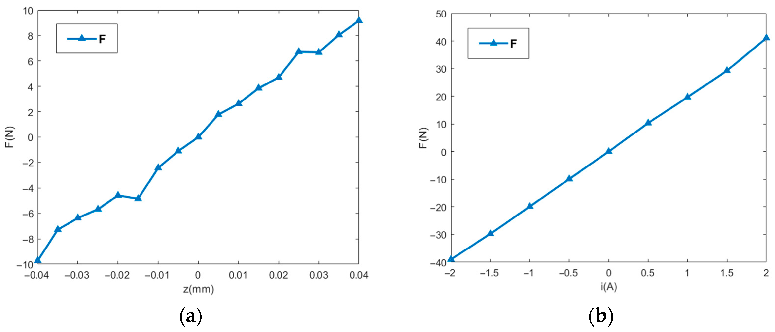
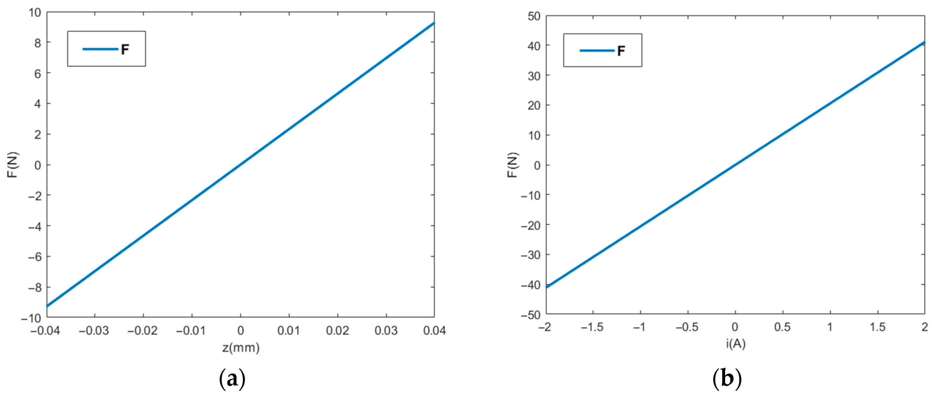
2.3. The Correlation between the Levitating Force and the Levitating Position of the MC

From Equations (33) and (34), it can be seen that the levitating force is related to both the upward offset of the MC and the planar position of the MC.

Let the current of the levitating coil be zero and the plane position y = 0, then Equations (33) and (34) can be transformed into:

$$F_{left}=-{({\displaystyle \frac{1}{0.1206-5.981\times z_l-1.9715\times z_r}})}^2+{({\displaystyle \frac{1}{0.1206+5.981\times z_l+1.9715\times z_r}})}^2$$

(35)

$$F_{right}=-{({\displaystyle \frac{1}{0.1206-1.9715\times z_l-5.981\times z_r}})}^2+{({\displaystyle \frac{1}{0.1206+1.9715\times z_l+5.981\times z_r}})}^2$$

(36)

From Equations (34) and (35), it can be seen that there is a cross-coupling between the levitating force on both sides of the MC and its upward offset.

When the left side of the MC moves upward, its left upward offset z_l increases, and the length of the upper left air gap decreases, which also decreases the length of the middle upper air gap, but the decrease is less than that of the left upper air gap. The decrease in two air gaps results in a decrease in two magnetic reluctance. Since the magnetic potentials of each magnetic loop remain unchanged, the magnetic fluxes of both loops increase, which is the increase in magnetic flux of loop 1 and loop 2, resulting in an increase in electromagnetic suction force on the upper left side. The decrease in the upper left air gap and the increase in the length of the lower left air gap result in an increase in the magnetic reluctance of the lower left air gap, which reduces the magnetic flux of loop 3, resulting in a decrease in electromagnetic suction force on the lower left side. Since the left levitating force is the sum of the upper electromagnetic suction force and the lower electromagnetic suction force on the left MC, an increase in z_l on the left side will result in an increase in levitating force on the left side. At the same time, an increase in magnetic flux of loop 2 results in an increase in electromagnetic suction force on the upper right side, while at this time, the length of the middle lower air gap and the left lower air gap increases, and magnetic flux of loop 3 decreases, resulting in a decrease in electromagnetic suction force on the lower right side. Therefore, the levitating force on the right side also increases upward. Since the upward offset z_r of the MC is less than that of the left side, z_l has a greater impact on the levitating force on the left side than on the right side. Similarly, z_r also has an impact on the levitating force on both sides of the MC. The influence of z_r on the right side levitating force is greater than that on the left side. Therefore, it can be seen that there is a strong coupling between the levitating forces on both sides of the MC and their upward offsets.

From Equations (32) and (33), it can be seen that the levitating forces on both sides of the MC are affected by the planar position y of the MC. From Equations (10)–(13), it can be seen that changes in the planar position y of the MC cause some changes in magnetic reluctance, resulting in changes in the magnetic flux of the eight magnetic loops, which ultimately lead to changes in the levitating forces on both sides of the MC.

The instantaneous upward offset and plane position changes of the MC can cause changes in relative magnetic permeability, but this is not included in the analytical model. To increase the precision of the model, it is necessary to use the actual curve instead of a linear approximation curve. However, this also increases the complexity of the analytical model and introduces more uncertainties.

The permanent magnet in the MR causes the magnetic loop to be in a magnetic saturation state, so that the magnetization point is only slightly affected by the upward shift and plane position changes of the MC. Therefore, the change in the relative magnetic permeability of the MR is also very small and can be almost ignored in engineering.

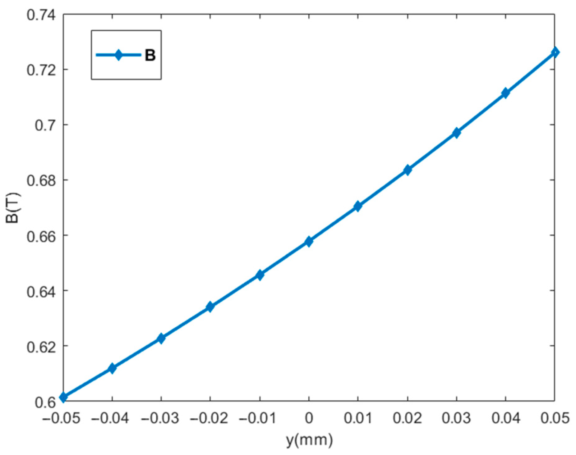
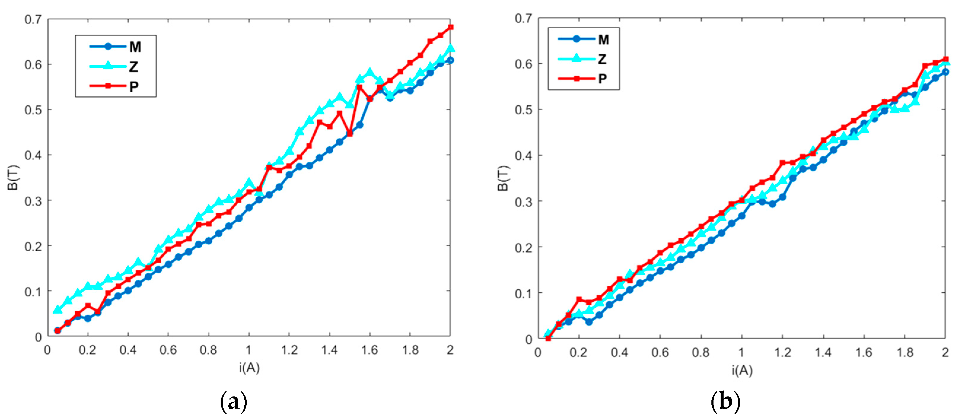
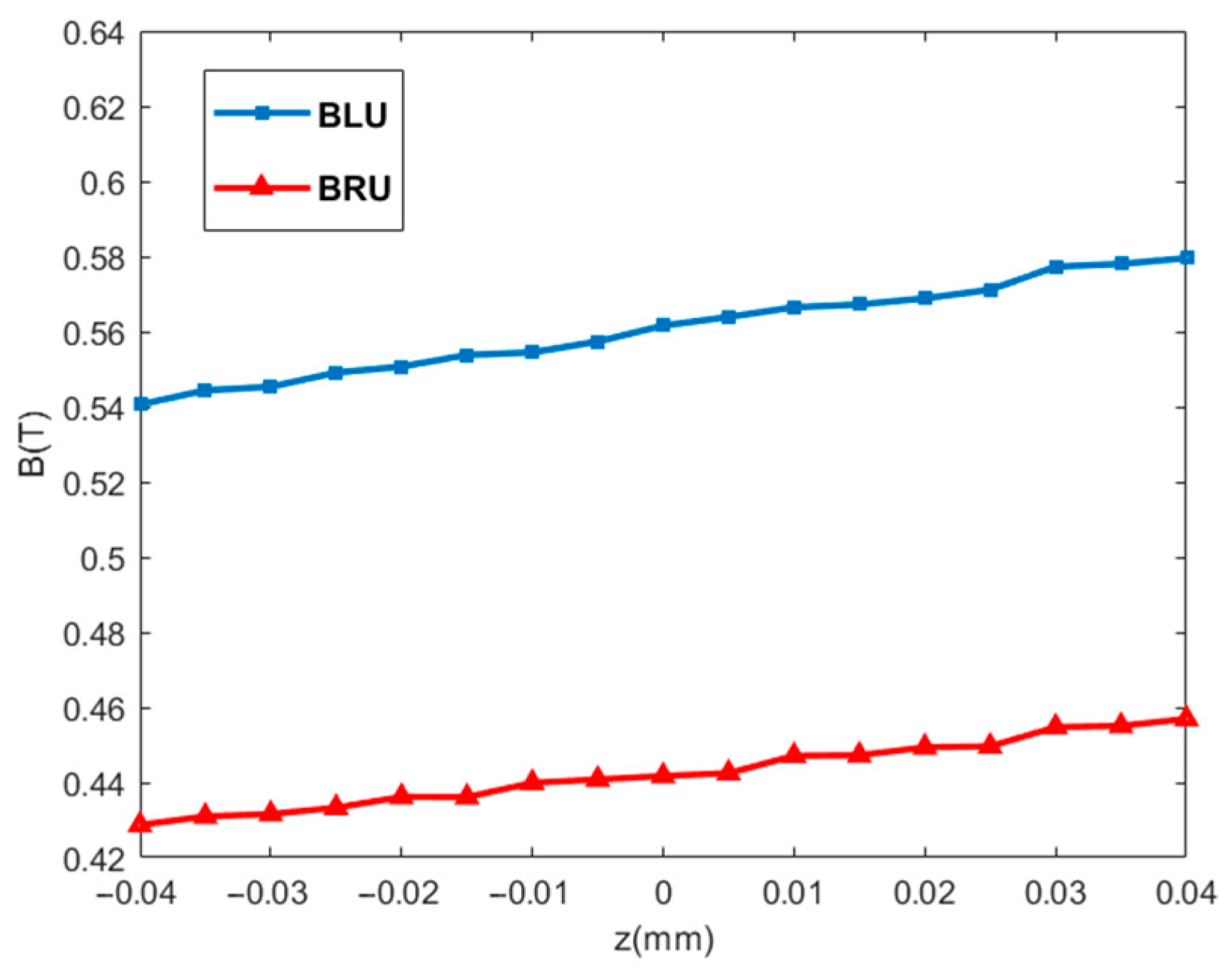
2.4. Verification of the Levitating Force Model and Magnetic Flux Leakage Parameters

It can be seen from the experiment that the change in the planar position of the MC will cause changes in the air gap flux [1]. From Equation (32), it can be seen that the air gap flux is the sum of the base levitating loop flux and the control levitating loop flux. In order to study the relationship between the planar position of the MC and the magnetic flux in air gaps, we can set i₁ = 0 A, z_l = z_r = 0 m, and substitute it into Equation (32), which can be calculated as follows:

$${\varphi }_{l\_up\_air}={\displaystyle \frac{1}{1.52\times {10}^4-2.85\times y\times {10}^4}}$$

(37)

By testing a corresponding set of air gap flux density values from y = −0.05 m to y = 0.05 m, a relationship curve between the plane position y and the air gap flux density was plotted, as shown in Figure 2.

When passing a current i₁ = 0~2 A through the upper left levitating coil, a set of upper left air gap flux density values was measured, and the relationship between the i₁ and the magnetic flux in the upper left air gap was plotted, as shown in Figure 3a.

When passing a current i₃ = 0~2 A through the upper right levitating coil, a set of upper right air gap flux density values were measured, and the relationship between the i₃ and the magnetic flux in the upper right air gap was plotted, as shown in Figure 3b.

The three colored lines in Figure 3, M, Z, and P, are data measured at the negative limit position, zero position, and positive limit position of the MC plane position.

The MC is temporarily fixed to the z-direction micro-motion platform, and adjust the height of the MC. The resolution of the z-direction micro-motion platform is 5 μm. The relationship between the height change of the MC and the air gap flux density can be detected. The detection conditions are that the current of the horizontal thrust coil i = 0 A and z_l = z_r. The detection results are shown in Figure 4.

The BLU curve in Figure 4 is the relationship between the magnetic flux in the upper left air gap and the levitation position of the MC; the BRU curve is the relationship between the magnetic flux in the upper right air gap and the levitation position of the MC. From Figure 4, it can be seen that changes in the air gap on the upper part of the MC will lead to changes in air gap flux density.

Static force detection still requires a z-direction micro-motion platform, with the MC temporarily fixed on the platform. A force sensor is added between the MC and the platform to detect the force applied to the MC.

During the detection process, the MC is first placed at the center of the plane, that is, at the plane position y = 0, to ensure uniformity of detection. Secondly, the levitating positions of the left and right ends of the MC are ensured to be the same, that is, z_l = z_r. Under the action of the magnetic field, if the levitation positions of the left and right ends of the MC are not the same, the levitating forces on the left and right ends of the MC will cross-couple and affect each other seriously.

Figure 5 shows the relationship between z and F_left, as well as ia and F_left. i_a = i₃ − i₁.

Next, the estimated values of the magnetic flux leakage system and the levitating force model are verified.

Equation (33) is obtained after substituting the leakage factor σ_BM = 6 of the basic levitation magnetic loop and controlling the leakage factor σ_CM = 3 of the levitation magnetic loop. The equation before substitution is as follows:

$$\begin{array}{l}{F}_{left}=-{\displaystyle \frac{({{\varphi }^2}_{l\_air\_up}-{{\varphi }^2}_{l\_air\_down})}{2{\mu }_0\cdot A}}=-9.95\times {10}^8\\ [({\displaystyle \frac{2650}{9.56\times {10}^6+\frac{3.42\times {10}^6}{{\sigma }_{BM}}-(8.87\times {10}^6\times y+\frac{2.98\times {10}^9\times z_l}{{\sigma }_{BM}}+\frac{0.99\times {10}^9\times z_r}{{\sigma }_{BM}})}}\\ +{\displaystyle \frac{N{i}_1}{6.14\times {10}^6+\frac{3.42\times {10}^6}{{\sigma }_{CM}}+8.94\times {10}^6\times y-\frac{2.98\times {10}^9\times z_l}{{\sigma }_{CM}}-\frac{0.99\times {10}^9\times z_r}{{\sigma }_{CM}}}}{)}^2\\ -({\displaystyle \frac{2650}{9.56\times {10}^6+\frac{3.42\times {10}^6}{{\sigma }_{BM}}-8.87\times {10}^6\times y+\frac{2.98\times {10}^9\times z_l}{{\sigma }_{BM}}+\frac{0.99\times {10}^9\times z_r}{{\sigma }_{BM}}}}\\ +{\displaystyle \frac{N{i}_3}{6.14\times {10}^6+\frac{3.42\times {10}^6}{{\sigma }_{CM}}+8.94\times {10}^6\times y+\frac{2.98\times {10}^9\times z_l}{{\sigma }_{CM}}+\frac{0.99\times {10}^9\times z_r}{{\sigma }_{CM}}}}{)}^2]\end{array}$$

(38)

In Equation (38), y = 0, i₁ = i₃ = 0, and z_l =z_r = z. Then, Equation (38) can be seen as F_left = f(z, σ_BM). Combining with Figure 6a, the least squares method can be used to estimate σ_BM = 6.1326. In addition, the leakage factor of the base levitation magnetic loop can also be estimated by using Figure 2 and the calculation equation for the magnetic flux $\varphi$₁ of the No. 1 magnetic loop. The estimated values obtained by the two methods are basically equal.

Then, substitute σ_BM = 6.1326 into Equation (38), set y = 0, z_l = z_r = 0, and set i_a = i₃ − i₁. Equation (38) can be seen as F_left = f(i_a, σ_BM), and then combined with Figure 5b, using the least squares method, it can be estimated that σ_CM = 2.8765.

Substituting the estimated leakage factor of the base levitating loop and the control levitating loop into Equation (38), the relationship between z and F_left can be obtained, as shown in Figure 6a, as well as the relationship between i_a and F_left, as shown in Figure 6b.

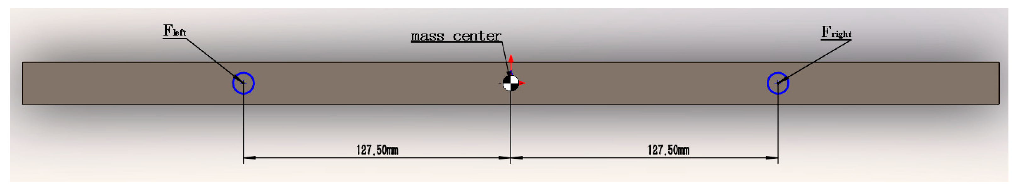
2.5. Dynamic Model of Levitating System

According to the analysis of electromagnetic suction force in Figure 1, the MC has two degrees of freedom in the levitating system: (1) vertical motion in the z-direction; (2) rotation around the y-axis with the center of mass of the MC as the center of rotation, denoted by ψ. This paper uses Newton’s second law of motion to describe the vertical motion of the MC and uses the torque equation to describe the rotational motion of the MC [18].

$$F=m\cdot {\displaystyle \frac{{\partial }^2{z}_a}{\partial t^2}}$$

(39)

$$M_{\alpha }=J_{\alpha }\cdot {\displaystyle \frac{{\partial }^2\alpha }{\partial t^2}}$$

(40)

In Equation (39), F is the sum of all forces on the MC in the z-direction, m is the mass of the MC, and z_a is the displacement of the mass center of the MC in the z-direction. In Equation (40), M_α is the torque of the resultant force of F, J_α is the moment of inertia, and α is the rotation angle. Figure 7 shows the position of the mass center, the force points of the levitating forces on the left and right ends of the MC, and the length of the arm of force.

$$J_{\alpha }=m_h{r}^2$$

(41)

In Equation (41), m_h is the mass of the mass center of the MC to the end, and r is the distance from the mass center to the point of action of the levitating force. From this, J_α can be calculated: J_α = 1.49 × 10⁻² kg∙m². Ignoring other disturbances, such as base vibration and horizontal thrust, the sum of all forces on the MC in the z-direction is:

$$F=-F_g+F_{left}+F_{right}$$

(42)

In Equation (42), F_g = mg = 17.93 N is the gravity force on the MC. From the dimensions indicated in Figure 7, the moment equation around the y-axis is as follows:

$$M_{\alpha }=-0.1275\times F_{left}+0.1275\times F_{right}$$

(43)

According to Equation (40), a new equation can be obtained:

$$-0.1275\times F_{left}+0.1275\times F_{right}=J_{\alpha }\cdot {\displaystyle \frac{{\partial }^2\psi }{\partial t^2}}$$

(44)

From Equations (39) and (42), a new equation can be obtained:

$$F_{left}+F_{right}-F_g=m\cdot {\displaystyle \frac{{\partial }^2{z}_a}{\partial t^2}}$$

(45)

Thus, the rigid body dynamics equation of the MC is obtained:

$$\left[\begin{array}{cc}1& 1\\ -0.1275& 0.1275\end{array}\right]\cdot \left[\begin{array}{c}{F}_{left}\\ F_{right}\end{array}\right]+\left[\begin{array}{c}17.93\\ 0\end{array}\right]=\left[\begin{array}{cc}1.83& 0\\ 0& 0.0273\end{array}\right]\left[\begin{array}{c}{\displaystyle \frac{{\partial }^2{z}_a}{\partial t^2}}\\ {\displaystyle \frac{{\partial }^2\psi }{\partial t^2}}\end{array}\right]$$

(46)

From Equations (33) and (34), it can be seen that F_left and F_right are related to z_l and z_r, which are in the [z_l, z_r] coordinate system with the air gap length as the research point. However, Equation (45) is in the [z_a, ψ] coordinate system with the mass center as the research point. A coordinate transformation is needed to convert the air gap length coordinate system to the mass center coordinate system.

As shown in Figure 1b, when the MC rotates around the y-axis, there is a relationship between z_l and z_r, the displacement of the mass center z_a, and the rotation angle ψ as follows:

$$z_l=z_a-0.1275\times \tan \psi$$

(47)

$$z_r=z_a+0.1275\times \tan \psi$$

(48)

Due to the very small length of the air gap, the rotation angle ψ is also very small, so tanψ≈ψ. Therefore, Equations (47) and (48) can be written as:

$$\left[\begin{array}{c}{z}_l\\ z_r\end{array}\right]=\left[\begin{array}{cc}1& -0.1275\\ 1& 0.1275\end{array}\right]\left[\begin{array}{c}{z}_a\\ \psi \end{array}\right]$$

(49)

The above equation can be used to convert the air gap length coordinate system into the centroid coordinate system. Since the left and right side levitating forces are two multivariable, nonlinear functions, the formula is very complex and requires approximate conversion. The conversion method is: (1) Assuming that the MC is at the zero point of the plane; (2) At the zero point of the levitation position, namely [z_l, z_r] = [0, 0], Taylor expansion is performed, and the high-order terms after the first term are truncated, resulting in simplified equations for the left and right end levitating forces of the MC as follows:

$$F_{left}=23.11\times i_{\mathrm{a}}-13600\times z_l-4483\times z_r$$

(50)

$$F_{right}=23.11\times i_b-4483\times z_l-13600\times z_r$$

(51)

In Equations (50) and (51), i_a = i₃ − i₁, and i_b = i₄ − i₂. i₁, i₂, i₃, and i₄ are the currents of the four levitating coils, respectively.

(3) Perform coordinate system transformation, and the transformation result is as follows:

$$F_{left}=23.11\times i_{\mathrm{a}}-18083\times z_a+1162.42\times \psi$$

(52)

$$F_{right}=23.11\times i_b-18083\times z_a-1162.42\times \psi$$

(53)

Substituting Equations (52) and (53) into Equation (46), the analysis model of the levitating system of the MR is obtained after sorting out:

$$\left[\begin{array}{cc}-36166& 0\\ 0& 296\end{array}\right]\left[\begin{array}{c}{z}_a\\ \psi \end{array}\right]+\left[\begin{array}{cc}23.11& 23.11\\ -2.9465& 2.9465\end{array}\right]\left[\begin{array}{c}{i}_a\\ i_b\end{array}\right]+\left[\begin{array}{c}17.93\\ 0\end{array}\right]=\left[\begin{array}{cc}1.83& 0\\ 0& 0.0273\end{array}\right]\left[\begin{array}{c}{\displaystyle \frac{{\partial }^2{z}_a}{\partial t^2}}\\ {\displaystyle \frac{{\partial }^2\psi }{\partial t^2}}\end{array}\right]$$

(54)

From Equation (54), it can be seen that the levitating system is a nonlinear system with two inputs and two outputs. Moreover, the system has strong coupling. Conventional linear algorithms cannot achieve effective control of the system. For the levitating system, ADRC is a more suitable controller.

3. A Levitating Control System Based on Active Disturbance Rejection

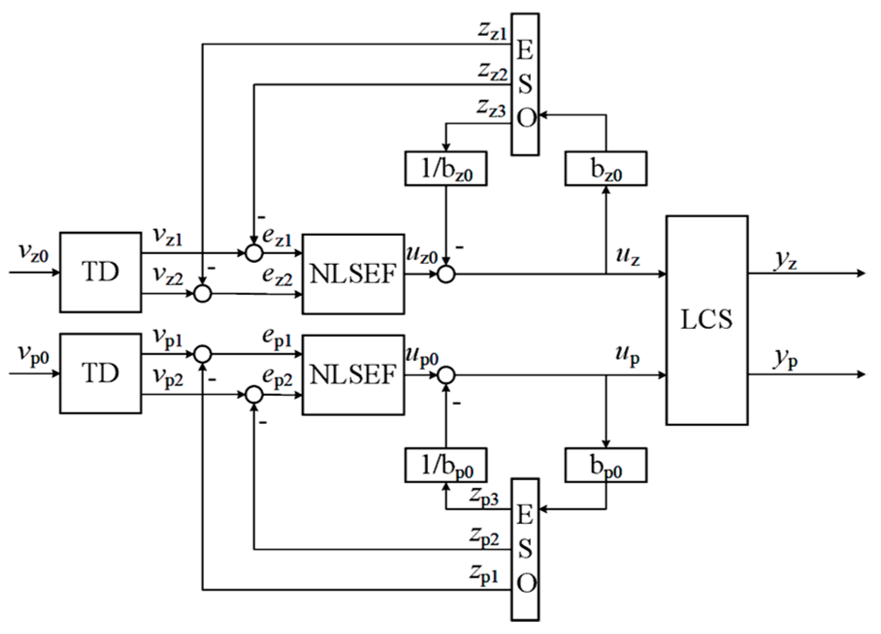
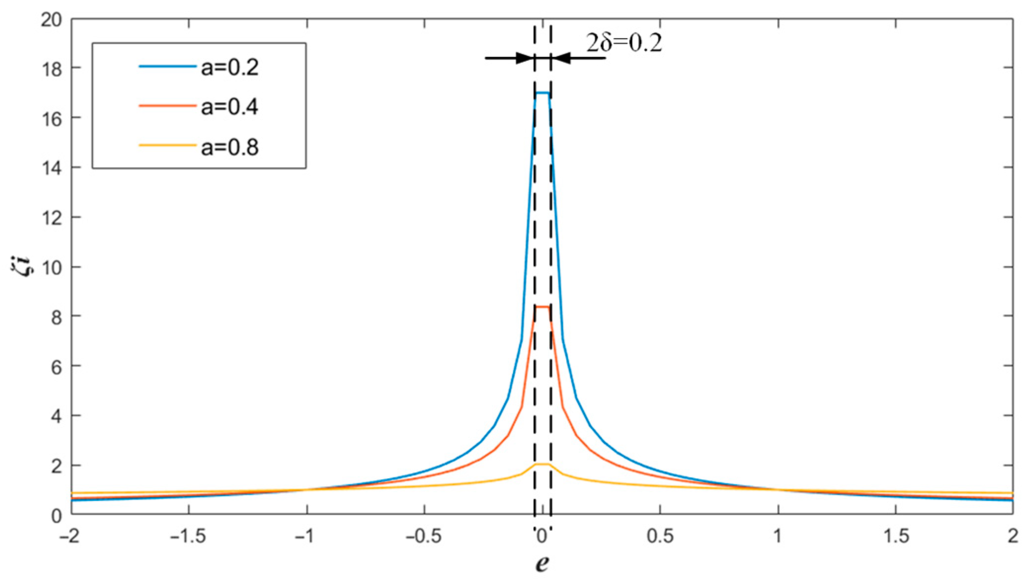
3.1. Design of Active Disturbance Rejection Controller for Levitating Control System

Based on an in-depth analysis of the PID control algorithms, Han Jingqing proposed the auto-disturbance rejection control technology [19]. This control technology does not require high precision in the mathematical model and can estimate and compensate for “internal disturbances” and “external disturbances” in the system in real time, with strong adaptability and good anti-interference performance [19,20].

Due to the susceptibility of the levitating system to working magnetic field, current, and load disturbances of the levitating coil, an active disturbance rejection control strategy is an effective solution to restrain the disturbances [19]. Because active disturbance rejection control not only requires lower modeling precision but also can observe and compensate for coupling disturbances between different degrees of freedom (z_a and ψ) through an extended state observer, thereby solving the decoupling and disturbance suppression problems in levitating control [19].

The ADRC controller of the levitating system is shown in Figure 8. It mainly consists of a tracking differentiator (TD), an extended state observer (ESO), and a nonlinear state error feedback control law (NLSEF) [20].

Han Jingqing proposed the concept of the nonlinear tracking differentiator, whose discrete tracking differentiator has the following form [2]:

1. Tracking differentiator (TD)

When the MR system is started, the given position will undergo a sudden change. However, due to inertia, the position of the MC will not immediately reach the given position, but there will be a relatively slow change process. This leads to the emergence of a transition process. When using the classical PID control algorithm for position control, if the z_a needs to track the v_z0 as soon as possible, the control quantity should be increased. However, after increasing the control quantity, the z_a will have an overshoot. The transition process of the z_a is an objective existence. Therefore, the best way to eliminate the overshoot is to arrange a transition process for the v_z0 [2].

The TD in the ADRC can be used to arrange a reasonable transition process for the given position. Equation (55) is a discretized second-order tracking differentiator [2].

$$\left\{\begin{array}{l}{v}_{z1}(n+1)=v_{\mathrm{z}1}(n)+h{v}_{z2}(n)\hfill \\ v_{z2}(n+1)=v_{z2}(n)+hfhan[v_{z1}(n)-v_{z0}(n),v_{z2}(n),r,h]\hfill \end{array}\right.$$

(55)

In the equation:

$$\begin{array}{l}fhan=\left\{\begin{array}{l}-rsign(\alpha ) \left|\alpha \right|>\delta \hfill \\ -r{\displaystyle \frac{\alpha }{\delta }} \left|\alpha \right|\le \delta \hfill \end{array}\right.\\ \alpha =\left\{\begin{array}{l}{v}_{\mathrm{z}2}(n)+{\displaystyle \frac{{\alpha }_0-\delta }{2}}sign(y_z(n)) \left|y_z(n)\right|>{\delta }_0\hfill \\ v_{z2}(n)+h{y}_z(n) \left|y_z(n)\right|\le {\delta }_0\hfill \end{array}\right.\\ {\alpha }_0=\sqrt{{\alpha }^2+8r\left|y_z(n)\right|}\\ \delta =r{h}_0\\ {\delta }_0=\delta h_0\\ y_z(n)=v_{z1}(n)-v_{z0}(n)+h_0{v}_{z2}(n)\end{array}$$

In the equation, v_z0(n) is the z_a initial signal, v_z1(n) traces the signal of v_z0(n), v_z2(n) is the differential signal of v_z0(n); h is the integration size of step, tracing speed is determined by r, and h₀ controls the effect of the noise filtering. r and h₀ should be coordinated to get a suitable transition process.

2. Extended State Observer (ESO)

According to the active disturbance rejection control law [21], Equation (53) is changed to:

$$\left\{\begin{array}{l}{\displaystyle \frac{{\partial }^2{z}_a}{\partial t^2}}=b_z{i}_a+w_z(t)\hfill \\ {\displaystyle \frac{{\partial }^2\Psi }{\partial t^2}}=b_p{i}_b+w_p(t)\hfill \end{array}\right.$$

(56)

In the equation, w_z(t) and w_p(t) are the equivalent disturbances of the system, which include coupling and disturbance. i_a and i_b are control variables. b_z and b_p in Equation (55) are the control parameters of control variables i_a and i_b. i_a = i₃ − i₁, i_b = i₄ − i₂. i₁, i₂, i₃, i₄ are the currents of the four levitating coils. Let Δi_a and Δi_b be the changes of i_a and i_b, respectively, then:

$$\left\{\begin{array}{l}{i}_a+\Delta i_a=(i_3+{\displaystyle \frac{\Delta i_a}{2}})-(i_1-{\displaystyle \frac{\Delta i_a}{2}})\hfill \\ i_b+\Delta i_b=(i_4+{\displaystyle \frac{\Delta i_b}{2}})-(i_2-{\displaystyle \frac{\Delta i_b}{2}})\hfill \end{array}\right.$$

(57)

After compensation, Equation (55) can be rewritten as:

$$\left\{\begin{array}{l}{\displaystyle \frac{{\partial }^2{z}_a}{\partial t^2}}=i_a^{*}\hfill \\ {\displaystyle \frac{{\partial }^2\Psi }{\partial t^2}}=i_b^{*}\hfill \end{array}\right.$$

(58)

After compensation, z_a and ψ are decoupled and controllable. Taking z_a as an example, it can be seen from Equation (53) that the system controls z_a through i_a. However, changes in i_a also cause changes in ψ, resulting in coupling. In Equation (55), after parameter adjustment, i_a becomes part of the equivalent disturbance of w_p(t), which is then observed and compensated by ESO. Similarly, controlling the other degree of freedom, i_b, also causes changes in z_a. In Equation (55), after parameter adjustment, i_b becomes part of the equivalent disturbance of w_z(t), and then ESO observes and compensates it. The ESO of the levitating system is as follows [2]:

$$\left\{\begin{array}{l}e(n)=z_1(n)-y_z(n)\hfill \\ z_1(n+1)=z_1(n)+h[z_2(n)-{\beta }_{e1}e(n)]\hfill \\ \begin{array}{c}{z}_2(n+1)=z_2(n)+h\left\{z_3(n)-{\beta }_{e2}fal[e(n),a_1,\delta ]+\right.\\ \left.b_0{u}_z(n)\right\}\end{array}\hfill \\ z_3(n+1)=z_3(n)-h{\beta }_{e3}fal[e(n),a_2,\delta ]\hfill \end{array}\right.$$

(59)

In the equation:

$$fal(e,a_j,\delta )=\left\{\begin{array}{l}{\left|e\right|}^{a_j}sign(e) \left|e\right|>\delta \hfill \\ {\displaystyle \frac{e}{{\delta }^{1-a_j}}} \left|e\right|\le \delta \hfill \end{array}\right.$$

In the equation: z₁(n), z₂(n), and z₃(n) are the state variables of the ESO, z₁(n) and z₂(n) are used to trace the state variables of the levitating system, and z₃(n) is used to trace the state variables of the total disturbance; β_e1, β_e2, and β_e3 are the gains of the ESO. a₁ and δ are undetermined parameters. If a_j is less than 1, the function has nonlinear characteristics; δ represents the linear range, aiming to avoid oscillation caused by large gain with minimal error.

3. Nonlinear error feedback control law (NLSEF)

In this paper, the levitating control system adopts the following form of NLSEF [2]:

$$\left\{\begin{array}{l}{e}_1(n+1)=w_1(n+1)-z_1(n+1)\hfill \\ e_2(n+1)=w_2(n+1)-z_2(n+1)\hfill \\ u_0(n+1)={\beta }_{f1}fal[e_1(n+1),a_3,{\delta }_{f1}]+\hfill \\ {\beta }_{f2}fal[e_2(n+1),a_4,{\delta }_{f1}]\hfill \end{array}\right.$$

(60)

In the equation, e₁(n) and e₂(n) are the deviations and derivatives between the expected transition process and the estimated value of the system output; a₂, a₃, and δ_f1 are the relevant parameters of fal; u₀ is the output of NLSEF; b₀ is the compensation coefficient.

4. Interference compensation [2]

Use ESO to track the variable z₃(n) expanded from the original system. Use the control variable to compensate for the disturbance. The control variable is:

$$u(n+1)={\displaystyle \frac{u_0(n+1)-z_3(n+1)}{b_0}}$$

(61)

After a large number of simulation experiments and prototype testing experiments [2], this paper summarizes the parameter tuning method for the levitating control system:

1. Parameter tuning of TD.

There are three parameters in TD that need to be tuned, namely r, h₀, and h.

r is the tracking factor. The tracking factor determines the speed at which w₁(n) and w₂(n) track the z_a given signal. The larger the tracking factor, the faster the tracing speed and the steeper the tracking curve. The smaller the tracking factor, the slower the tracing speed and the slower the tracking curve. However, it is also necessary to set a suitable tracking factor value based on the inertia of the MC to ensure the tracing effect of w₁(n) and w₂(n). h₀ is the filtering factor. The effect of TD is determined by the h₀. h₀ is related to the execution frequency of the controller [2]. h is the integration step size [2]. The shorter the integration step size, the higher the precision of the integral value, but the stronger the lag. An overly short integration step size can cause system oscillations. However, an overly long integration step size can reduce the precision of the integral value. In this paper, h = h₀.

2. Parameter tuning of ESO.

By analyzing the inherent laws of ESO parameters and referring to the bandwidth method [22], this section proposes an ESO parameter tuning method for the levitation control system.

Suppose:

$$fal(e, a_j, \delta )={\displaystyle \frac{fal(e, a_j, \delta )}{e}}e={\zeta }_i(e)e$$

(62)

where i = 1, 2. Substituting Equation (62) into Equation (59):

$$\left\{\begin{array}{l}e=z_1-y_z\hfill \\ {\dot{z}}_1=z_1+h\left(z_2-{\beta }_{e1}e\right)\hfill \\ {\dot{z}}_2=z_2+h\left[z_3-{\beta }_{e2}{\zeta }_1(e)e+b_0{u}_z\right]\hfill \\ {\dot{z}}_3=z_3-h{\beta }_{e3}{\zeta }_1(e)e\hfill \end{array}\right.$$

(63)

In order to analyze the characteristics of the function ζ_i(e) and compare the changes in the output of the function ζ_i(e) corresponding to different a_j values, this article selects a_j = 0.2, a_j = 0.4, a_j = 0.8, and δ = 0.1, resulting in the output curve of the function ζ_i(e) shown in Figure 9.

From Figure 9, it can be seen that as the a_j decreases, the nonlinearity of function ζ_i(e) increases, and the maximum gain increases. It can be seen that too small a_j may lead to high-frequency oscillations in the observed values, while a larger a_j may make it difficult for ESO to leverage its advantages of fast error attenuation and strong anti-interference capabilities. That is to say, a_j can significantly affect the performance of ESO. In addition, if the error e is within the range [−δ, δ], the function ζ_i(e) is a constant, and ${\left({\zeta }_i\left(e\right)\right)}_{\max }={\delta }^{a_j-1}$. Additionally, an excessively large linear interval δ can cause the nonlinear gain to fail, while a δ that is too small can render the observer unstable. Typically, δ should fall within the range of [0.001, 0.1], with δ = h being suitable in this context; a_j must satisfy the condition that a₁ > a₂. According to the empirical values, a₁ = 0.5 and a₂ = 0.25.

In ESO, there are three additional parameters that require adjustment, namely β_e1, β_e2, and β_e3. β_e3 is the most important of the three parameters. When tuning the parameters, first select the parameter β_e3. If β_e3 is too small, it will cause insufficient observation precision of z₃(n), and z₁(n) and z₂(n) will lag behind w₁(n) and w₂(n). If β_e3 is too large, it will cause increased system fluctuations and even system oscillations. Therefore, adjust β_e3 first to ensure the precision of ESO, and then adjust β_e1 and β_e2 from small to large to reduce the oscillation of ESO output. Due to the coupling of the levitating system, these two parameter values should be as small as possible while ensuring stable ESO output.

This paper employs the bandwidth method and experimental approach to tune the parameters of ESO. Therefore, based on the optimal parameter settings obtained through simulation in reference [2,23], the tuning formulas for β_e1, β_e2, and β_e3 proposed in this paper can be expressed as follows:

$${\beta }_{e1}=2{\omega }_0, {\beta }_{e2}={\displaystyle \frac{7{\omega }_0^2}{50}}, {\beta }_{e3}={\displaystyle \frac{{\omega }_0^3}{1000}}$$

(64)

Consequently, the performance of ESO is influenced by ω₀. Performing the Laplace transform on Equation (63) yields:

$$\left\{\begin{array}{l}e=z_1-y_z\hfill \\ s{z}_1=z_1+h\left(z_2-{\beta }_{e1}e\right)\hfill \\ s{z}_2=z_2+h\left[z_3-{\beta }_{e2}{\zeta }_1(e)e+b_0{u}_z\right]\hfill \\ s{z}_3=z_3-h{\beta }_{e3}{\zeta }_1(e)e\hfill \end{array}\right.$$

(65)

According to Equation (65), the transfer function model is obtained as:

$$z_1={\displaystyle \frac{({\beta }_{e2}{h}^2{b}_0{u}_z+{\beta }_{e2}{h}^2{y}_z{\zeta }_1(e))(s-1)+{\beta }_{e3}{h}^3{y}_z{\zeta }_2(e)+{\beta }_{e1}h{y}_z{(s-1)}^2}{s^3+({\beta }_{e1}h-3)s^2+({\beta }_{e2}{h}^2{\zeta }_1(e)+3-2{\beta }_{e1}h)s+{\beta }_{e1}h-1+{\beta }_{e3}{\zeta }_2(e)h^3-{\beta }_{e2}{\zeta }_1(e)h^2}}$$

(66)

$$\begin{array}{l}{z}_2={\displaystyle \frac{((b_0{\beta }_{e2}h{u}_z+{\beta }_{e2}h{y}_z{\zeta }_1(e))(s-1)+{\beta }_{e3}{h}^2{\zeta }_2(e)y_z)(s+{\beta }_{e1}h-1)}{s^3+({\beta }_{e1}h-3)s^2+({\beta }_{e2}{h}^2{\zeta }_1(e)+3-2{\beta }_{e1}h)s+{\beta }_{e1}h-1+{\beta }_{e3}{\zeta }_2(e)h^3-{\beta }_{e2}{\zeta }_1(e)h^2}}-\\ {\displaystyle \frac{{\beta }_{1}h{y}_z({\beta }_3{h}^2{\zeta }_2(e)+{\beta }_{2}h{\zeta }_1(e)(s-1))}{s^3+({\beta }_{e1}h-3)s^2+({\beta }_{e2}{h}^2{\zeta }_1(e)+3-2{\beta }_{e1}h)s+{\beta }_{e1}h-1+{\beta }_{e3}{\zeta }_2(e)h^3-{\beta }_{e2}{\zeta }_1(e)h^2}}\end{array}$$

(67)

$$\begin{array}{l}{z}_3={\displaystyle \frac{({\beta }_{e3}h{\zeta }_2(e)y_z({\beta }_{e2}{h}^2{\zeta }_1(e)+{\beta }_{e1}h(s-1)+{(s-1)}^2))}{s^3+({\beta }_{e1}h-3)s^2+({\beta }_{e2}{h}^2{\zeta }_1(e)+3-2{\beta }_{e1}h)s+{\beta }_{e1}h-1+{\beta }_{e3}{\zeta }_2(e)h^3-{\beta }_{e2}{\zeta }_1(e)h^2}}-\\ {\displaystyle \frac{{\beta }_{e3}{h}^2{\zeta }_2(e)(b_0{\beta }_{e2}h{u}_z+{\beta }_{e2}h{\zeta }_1(e)y_z)}{s^3+({\beta }_{e1}h-3)s^2+({\beta }_{e2}{h}^2{\zeta }_1(e)+3-2{\beta }_{e1}h)s+{\beta }_{e1}h-1+{\beta }_{e3}{\zeta }_2(e)h^3-{\beta }_{e2}{\zeta }_1(e)h^2}}-\\ {\displaystyle \frac{{\beta }_{e1}{\beta }_{e3}{h}^2{\zeta }_2(e)y_z(s-1)}{s^3+({\beta }_{e1}h-3)s^2+({\beta }_{e2}{h}^2{\zeta }_1(e)+3-2{\beta }_{e1}h)s+{\beta }_{e1}h-1+{\beta }_{e3}{\zeta }_2(e)h^3-{\beta }_{e2}{\zeta }_1(e)h^2}}\end{array}$$

(68)

According to Equation (66), ESO exhibits superior suppression of disturbances to u_z. However, the effectiveness in suppressing disturbances introduced by y_z requires further analysis. Hence, the effects of u_z interference and nonlinear factors can be disregarded to simplify the analysis; setting u_z = 0, ζ₁(e) = ζ₂(e) = 1, and then substituting Equation (64) into (66) yields:

$${\displaystyle \frac{z_1}{y_z}}={\displaystyle \frac{2{\omega }_0{s}^2+(0.14\times {10}^{-3}{\omega }_0^2-4{\omega }_0)s+{10}^{-6}{\omega }_0^3-0.14\times {10}^{-3}{\omega }_0^2+2{\omega }_0}{1000s^3+(2{\omega }_0-3)s^2+(0.14\times {10}^{-3}{\omega }_0^2-4{\omega }_0+3)s+{10}^{-6}{\omega }_0^3-0.14\times {10}^{-3}{\omega }_0^2+2{\omega }_0-1000}}$$

(69)

With the increase in ω₀, the ESO exhibits better dynamic performance, evidenced by more precise disturbance estimation, reduced phase lag in disturbance observation, and accelerated convergence of estimation error. However, the influence of a broad bandwidth on high-frequency noise is significant and cannot be overlooked, potentially resulting in a decline in the suspension control system’s performance. Therefore, in practical applications, it is advisable to adjust ω₀ gradually until the disturbance observation satisfies the requirements of system.

3. Parameter tuning of NLSEF.

Three parameters of NLSEF needed to be tuned, namely β_f1, β_f2, and b₀. b₀ is the coefficient of the control variable u. The adjustment methods for β_f1 and β_f2 are similar to those for PD parameters.

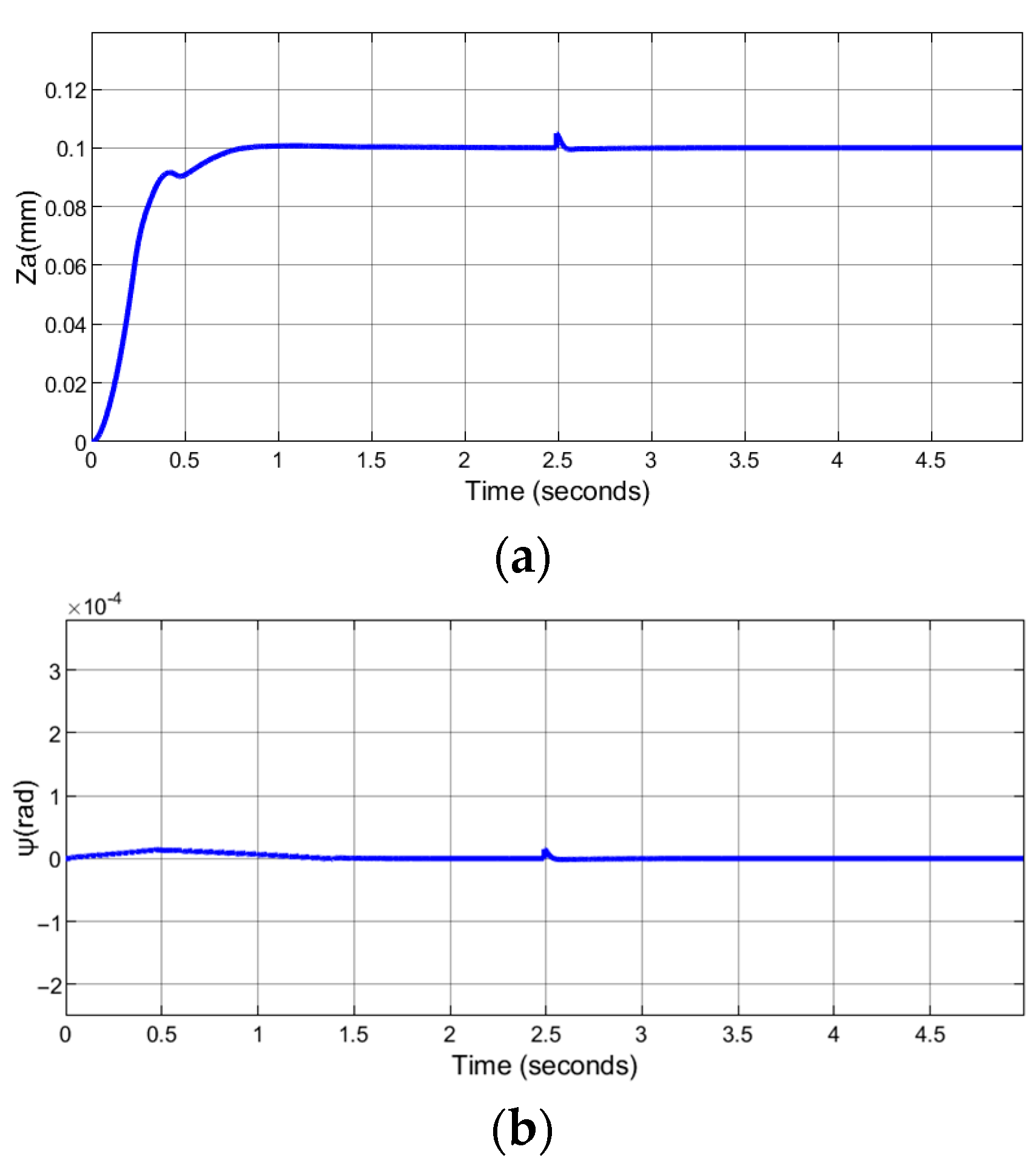
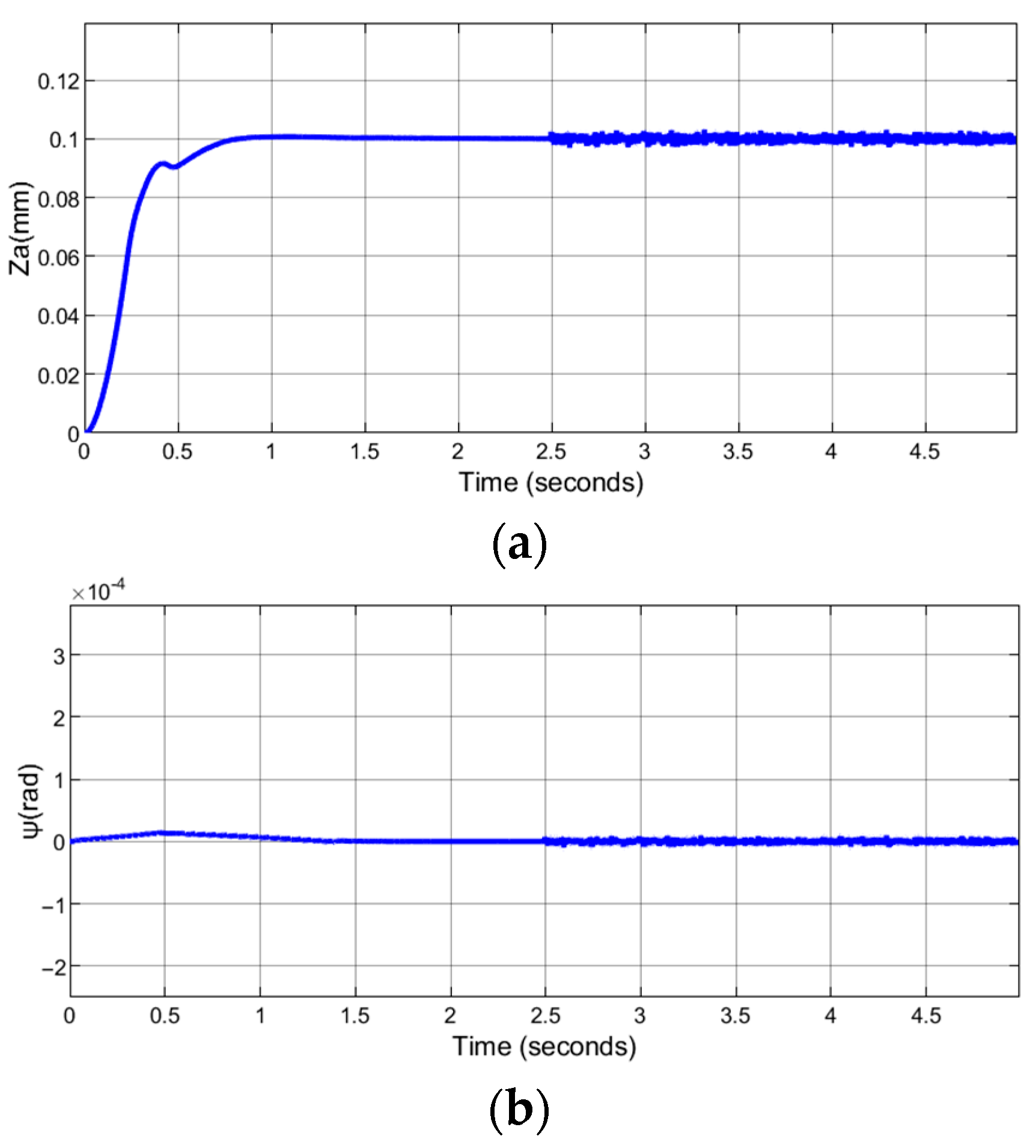
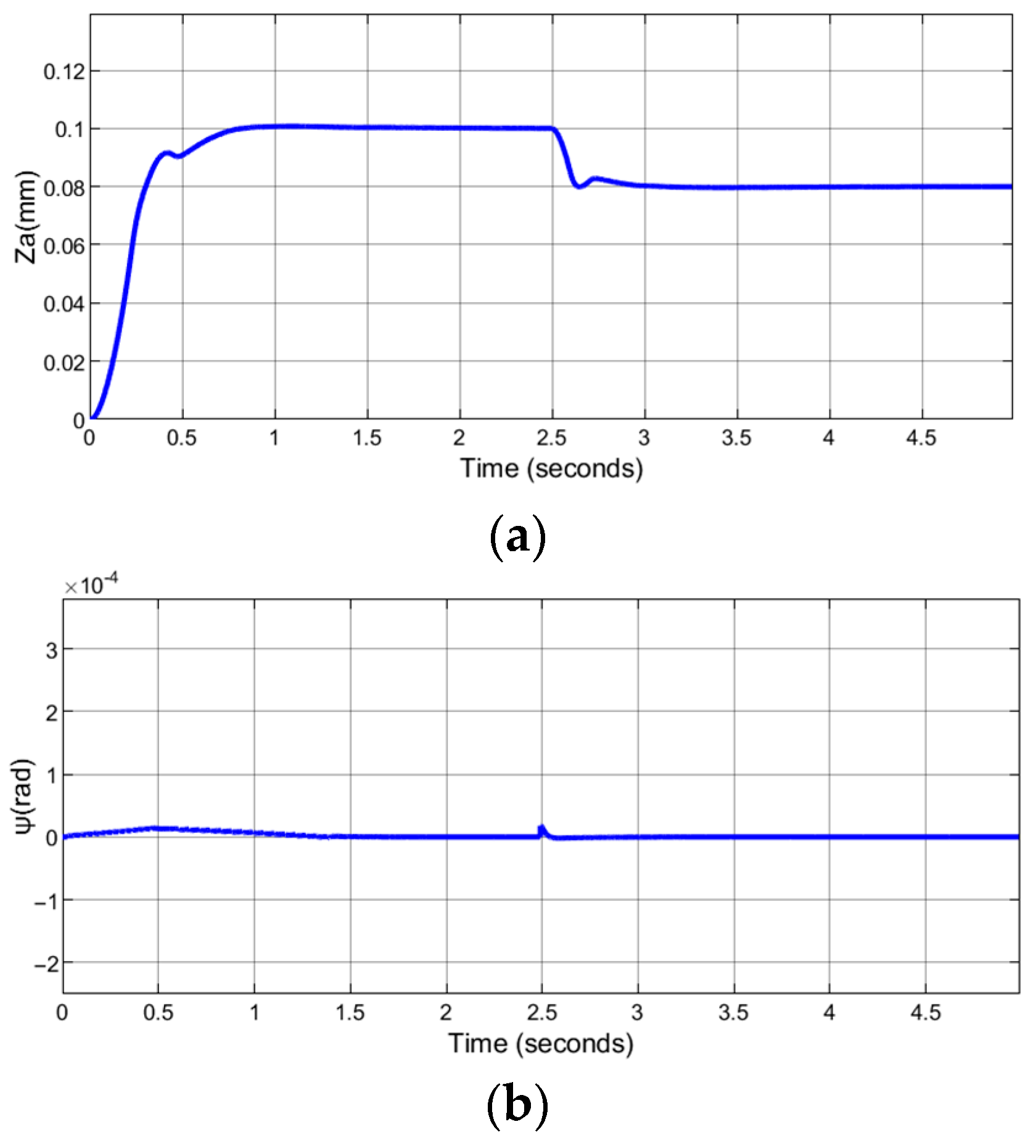
3.2. Simulation Analysis of the Levitating Control System

In order to facilitate the simulation analysis of the feasibility of the levitating control system, a simulation model of the levitating control system was built using Simulink, as shown in Figure 10.

The parameters of the MC are: J_α = 1.49 × 10⁻² kg∙m², r = 0.1275 m, and mass m = 1.83 kg. The parameters of ADRC are shown in

Table 2. Main parameters of ADRC.

Parameter	Value	Parameter	Value	Parameter	Value
r	900	βe2	1398	βf2	0.01
h	0.001	βe3	1015	a2	0.25
βe1	200	βf1	30	a3	0.5

.

When t = 0 s and the y-direction coordinate value of the MC is 0, a given value z*_a = 0.1 mm is suddenly applied with ψ* = 0 rad/s to detect the response characteristics of the levitating system during system startup.

In addition, when the MC moves along the y-axis, the magnetic field in air gaps will fluctuate, causing changes in the levitating position [1]. Therefore, at t = 2.5 s, a position disturbance with z_a = 0.008 mm is used to replace the fluctuation of the magnetic field in air gaps to simulate the disturbance to the levitating system. The simulation results are shown in Figure 11.

As shown in Figure 11, when the system started, the mover core reached the equilibrium position within 1 s without overshooting. The angle change in the mover core was also very small. The disturbance that occurred at 2.5 s had little effect on the levitation position of the mover core. The position change was less than 0.008 mm. The disturbance also had little effect on the angle of the mover core.

Next, the levitating control system was subjected to a system stability test by adding white noise with an amplitude of 0.5 at t = 2.5 s to simulate external interference. The simulation results are shown in Figure 12.

As can be seen from Figure 12, the white noise that appears at 2.5 s is a high-frequency interference signal that had little effect on the levitation position of the mover core and had little effect on the angle of the mover core. The levitation system can overcome the high-frequency interference simulated in the experiment.

Finally, at t = 2.5 s, the system setting was suddenly changed from 0.1 mm to 0.08 mm, and then a stability test was conducted. The simulation results are shown in Figure 13.

As shown in Figure 13, there was a sudden change in the set point of the system at 2.5 s. The mover core stabilized at a new position within 0.5 s. Although there was an overshoot during the process, the magnitude of the overshoot was less than 0.005 mm, which met the system requirements.

As can be seen from Figure 11, Figure 12 and Figure 13, the response curve of the levitating control system is relatively smooth, with a relatively small fluctuation amplitude.

4. Experimental Testing of the Levitating Control System

To confirm the effectiveness of the MR’s levitating control system, this paper conducted experimental testing of the levitating control using the hardware platform shown in Figure 14.

The hardware platform comprised an MR [1], levitating control coil, DC/DC converter, sensors, and a data collector. The levitating height sensor was securely mounted on the stator yoke and utilized a clamping mechanism. z_a in the Figure 15 was captured by levitating height sensor. The angle sensor is affixed to the mover core using an adhesive. ψ in Figure 15 was captured by an angle sensor. The gathered data was transmitted to the data collector via the bus. The data collector employed the Kalman filtering technique to eliminate invalid data.

Figure 15 is the measured start-up response curve of the MC.

As shown in Figure 15a, the levitating position setting value of the MC was adjusted to increase by 0.1 mm upward at t = 1 s. The levitating position of the MC reached the set value within 0.75 s, with no significant overshoot. After 0.75 s, the levitating position of the MC stabilizes at the set levitating position value; the error is within ±2 μm. It can be seen that the independent control of the four air gap magnetic fields makes the levitating control system of the MR have characteristics of small overshoot, fast following of the given value, good stability, and few oscillation times, with good dynamic and static characteristics.

As shown in Figure 15b, the angle of the MC deflected at t = 1 s. At this moment, the set value of the levitating position of the MC also underwent a sudden change, and the levitating control system began to adjust the levitating position of the MC. At t = 1.5 s, the deflection angle attained its maximum, and during the interval from t = 1 s to t = 1.5 s, the slope of the curve depicting the levitating position of the MC exhibited its steepest incline. After t = 1.5 s, the levitating position of the MC approached and reached the set levitating position, and the deflection angle also continuously decreased. Before t = 2.5 s, the deflection angle returned to zero degrees, and the transition process of the levitating position was also completed, with the MC stabilized at the new levitating position. It is evident that there exists a strong coupling in controlling the levitating positions of the left and right ends of the MC. The transitional process of the levitating position introduces disturbances to the angle of the MC. Nevertheless, the levitating control system promptly mitigates these disturbances. Consequently, the levitating control system effectively achieves decoupling control and possesses excellent robustness.

5. Discussion

The levitating system of the MR is characterized as a nonlinear, strongly coupled, and inherently unstable system. This paper establishes a mathematical model of the levitating system through magnetic circuit analysis and force analysis, revealing the relationship between the current of the levitating control coil and the air gap magnetic field, as well as the levitating height (z_a) and angle (ψ) of the MR. It also reveals the principle of strong coupling of the levitating system and converts the levitating system from a four-input, two-output system to a two-input, two-output system, proposing a levitating control system based on ADRC.

In the literature [1], the selection of magnetic circuit components and parameter settings for the MR were designed, and a large number of experiments were conducted to demonstrate that the four air gap magnetic fields can be independently controlled, as well as the fluctuation range of the levitating force of the MC at different positions. Based on the literature [1], this paper establishes a mathematical model of the suspension system through magnetic circuit analysis and force analysis. From Equations (50) to (54), it can be seen that there is a coupling between the suspension heights at both ends of the mover core, and the suspension system is a second-order system, not a typical linear system. These are not proposed in the literature [1].

The standard ADRC controller is capable of controlling second-order systems and decoupling effectively [2,12,19,20,21]. However, the levitating system of the MR is a four-input two-output system, which is different from the system in the literature. This paper simplifies the levitating system into a two-input two-output system using Equations (50) and (51). And improvements have been made to the ESO of ADRC, as shown in Equation (57). The improved ADRC can be applied to the suspension system of magnetic levitation rulers. Through simulation and experiments, it has been proven that the suspension control system of the magnetic levitation ruler can quickly follow the set value, effectively suppress sudden interference and white noise, have small overshoot, and have good dynamic and static characteristics as well as robustness.

In addition, classical PID controllers cannot achieve decoupling control and cannot be applied in four-input, two-output systems.

6. Conclusions

This paper first establishes a mathematical model of the levitating system of the MR, theoretically revealing the relationship between the current of the levitating control coil and the position and rotation angle of the MC and the suspension height between the two ends of the mover iron core. It further elucidates the coupling relationship between the levitating heights at both ends of the MC. In addition, the levitating system is simplified to a dual-input, dual-output system. The levitating system is a nonlinear and strongly coupled system. Classical PID control methods cannot achieve decoupling control. Therefore, a levitating controller based on ADRC is proposed. The ESO of ADRC has been improved to adapt to the simplified levitating system.

Simulation analysis and experimental testing through system startup, interference addition, white noise addition, and given sudden changes indicate that the levitating control system can quickly track changes in the setpoint, effectively suppress interference, have a small overshoot, and exhibit good dynamic and static characteristics as well as robustness. The levitating control system can ensure the stability of the levitating position of the MC, thereby ensuring the stability of the four air gap magnetic fields.

References

1. Sun, J.-Y.; Li, P.; Zheng, Y.; Tian, C.-L.; Zhou, Z.-Z. A novel magnetic circuit and structure for magnetic levitation ruler. Meas. Control 2023, 56, 1545–1561. [Google Scholar] [CrossRef]
2. Zhou, Z.-Z.; Wang, H.-X.; Liu, B.-S. Levitation position control of a precise 6-DOF Planar magnetic Levitation stage. Mach. Tool Hydraul. 2018, 46, 125–131. [Google Scholar] [CrossRef]
3. Liu, L.-L.; Zhou, J.-H. Parameter Self-adjusting Control Method of Fuzzy PID for Magnetic Levitation Ball System. Control Eng. China 2021, 28, 354–359. [Google Scholar] [CrossRef]
4. Hernández-Guzmán, V.M.; Silva-Ortigoza, R.; Marciano-Melchor, M. Position Control of a Maglev System Fed by a DC/DC Buck Power Electronic Converter. Complexity 2020, 2020, 8236060. [Google Scholar] [CrossRef]
5. Debdoot, S. Real-Time implementation and performance analysis of robust 2-DOF PID controller for Maglev system using pole search technique. J. Ind. Inf. Integr. 2019, 15, 183–190. [Google Scholar] [CrossRef]
6. Aysen, D.; Serdar, E.; Baran, H.; Davut, I. Opposition-based artificial electric field algorithm and its application to FOPID controller design for unstable magnetic ball levitating system. Eng. Sci. Technol. Int. J. 2021, 24, 469–479. [Google Scholar] [CrossRef]
7. Chauhan, D.; Yadav, A. Stability and agent dynamics of artificial electric field algorithm. J. Supercomput. 2024, 80, 835–864. [Google Scholar] [CrossRef]
8. Deepa, T.; Subbulekshmi, D.; Lakshmi, P.; Maheedhar, M.; Kishore, E.; Vinodharanai, M.; Chockalingam, T. Comparative Study of Different Controllers for Levitating Ferromagnetic Material. Adv. Mater. Sci. Eng. 2022, 2022, 4344083. [Google Scholar] [CrossRef]
9. Pandey, S.; Dourla, V.; Dwivedi, P.; Junghare, A. Introduction and realization of four fractional-order sliding mode controllers for nonlinear open-loop unstable system: A magnetic levitation study case. Nonlinear Dyn. 2019, 98, 601–621. [Google Scholar] [CrossRef]
10. Yaseen, H.M.S.; Siffat, S.A.; Ahmad, I.; Malik, A.S. Nonlinear adaptive control of magnetic levitation system using terminal sliding mode and integral backstepping sliding mode controllers. ISA Trans. 2022, 126, 121–133. [Google Scholar] [CrossRef]
11. Acharya, D.S.; Swain, S.K.; Mishra, S.K. Real-Time Implementation of a Stable 2 DOF PID Controller for Unstable Second-Order Magnetic Levitation System with Time Delay. Arab. J. Sci. Eng. 2020, 45, 6311–6329. [Google Scholar] [CrossRef]
12. Gopi, R.S.; Srinivasan, S.; Panneerselvam, K.; Teekaraman, Y.; Kuppusamy, R.; Urooj, S. Enhanced Model Reference Adaptive Control Scheme for Tracking Control of Magnetic Levitation System. Energies 2021, 14, 1455. [Google Scholar] [CrossRef]
13. Kim, S.K.; Ahn, C.K. Sensorless non-linear position-stabilising control for magnetic levitation systems. IET Control. Theory Appl. 2020, 14, 2682–2687. [Google Scholar] [CrossRef]
14. Zhu, H.; Teo, T.J.; Pang, C.K. Magnetically Levitated Parallel Actuated Dual-Stage (Maglev-PAD) System for Six-Axis Precision Positioning. IEEE/ASME Trans. Mechatron. 2019, 24, 1829–1838. [Google Scholar] [CrossRef]
15. Trbusic, M.; Jesenik, M.; Trlep, M.; Hamler, A. Energy Based Calculation of the Second-Order Levitation in Magnetic Fluid. Mathematics 2021, 9, 2507. [Google Scholar] [CrossRef]
16. Li, Y.-Q.; Feng, G.-S.; Wang, X.-F.; Wu, J.-Z.; Ma, J.; Xiao, L.-T.; Jia, S.-T. Reduction of characteristic RL time for fast, efficient magnetic levitation. AIP Adv. 2017, 7, 095016. [Google Scholar] [CrossRef]
17. Wu, C.; Li, S.-S. Modeling, Design and Suspension Force Analysis of a Novel AC Six-Pole Heteropolar Hybrid Magnetic Bearing. Appl. Sci. 2023, 13, 1643. [Google Scholar] [CrossRef]
18. Chen, W.; Tong, J.-Q.; Yang, H.-H.; Liu, F.-L.; Qin, Z.; Ren, Z.-Y. Modeling and Vibration Analysis of a 3-UPU Parallel Vibration Isolation Platform with Linear Motors Based on MS-DT-TMM. Shock. Vibation 2021, 2021, 9918097. [Google Scholar] [CrossRef]
19. Yu, T.-T.; Zhang, Z.-Z.; Li, Y.; Zhao, W.-L.; Zhang, J.-C. Improved active disturbance rejection controller for rotor system of magnetic levitation turbomachinery. Electron. Res. Arch. 2023, 31, 1570–1586. [Google Scholar] [CrossRef]
20. Tan, L.-L.; Chen, Z.-X.; Gao, Q.-H.; Liu, J.-F. Performance recovery of uncertain nonaffine systems by active disturbance rejection control. Meas. Control 2024, 57, 3–15. [Google Scholar] [CrossRef]
21. Sun, X.-D.; Jin, Z.-J.; Chen, L.; Yang, Z.-B. Disturbance rejection based on iterative learning control with extended state observer for a four-degree-of-freedom hybrid magnetic bearing system. Mech. Syst. Signal Process. 2021, 153, 107465. [Google Scholar] [CrossRef]
22. Wei, Z.-X.; Huang, Z.-W.; Zhu, J.-M. Position Control of Magnetic Levitation Ball Based on an Improved Adagrad Algorithm and Deep Neural Network Feedforward Compensation Control. Math. Probl. Eng. 2020, 2020, 8935423. [Google Scholar] [CrossRef]
23. He, H.-C.; Si, T.-T.; Sun, L.; Liu, B.-T.; Li, Z.-B. Linear Active Disturbance Rejection Control for Three-Phase Voltage-Source PWM Rectifier. IEEE Access 2020, 8, 45050–45060. [Google Scholar] [CrossRef]
Figure 1. (a) Magnetic loops of MR. (b) The electromagnetic suction force on the MC.
Applsci 14 08069 g001
Figure 2. The relationship between y and the air gap flux.
Applsci 14 08069 g002
Figure 3. The relationship between i3 and the air gap flux: (a) in upper left air gap; (b) in upper right air gap.
Applsci 14 08069 g003
Figure 4. The relationship between z and ϕ l_up_air and ϕ R_up_air.
Applsci 14 08069 g004
Figure 5. (a) The relationship between z and Fleft. (b) The relationship between ia and Fleft.
Applsci 14 08069 g005
Figure 6. (a) The calculation relationship between z and Fleft. (b) The calculation relationship between ia and Fleft.
Applsci 14 08069 g006
Figure 7. Force analysis of the MC.
Applsci 14 08069 g007
Figure 8. Structural diagram of levitating system.
Applsci 14 08069 g008
Figure 9. Comparison of the output of function ζi(e) corresponding to different aj.
Applsci 14 08069 g009
Figure 10. Simulation diagram of levitating control system.
Applsci 14 08069 g010
Figure 11. Simulation diagram of levitating control system. (a) Position variation curve. (b) Angle variation curve.
Applsci 14 08069 g011
Figure 12. Simulation diagram of external interference. (a) Position variation curve. (b) Angle variation curve.
Applsci 14 08069 g012
Figure 13. Simulation diagram of sudden change. (a) Position variation curve. (b) Angle variation curve.
Applsci 14 08069 g013
Figure 14. The measurement platform of the levitating system.
Applsci 14 08069 g014
Figure 15. System response curve during startup. (a) Position variation curve. (b) Angle variation curve.
Applsci 14 08069 g015