Abstract
This paper proposes a parameter optimization method for a terminal sliding mode controller (TSMC) based on a multi-strategy improved crayfish algorithm (JLSCOA) to enhance the performance of ship dynamic positioning systems. The TSMC is designed for the “Xinhongzhuan” vessel of Dalian Maritime University. JLSCOA integrates subtractive averaging, Levy Flight, and sparrow search strategies to overcome the limitations of traditional crayfish algorithms. Compared to COA, WOA, and SSA algorithms, JLSCOA demonstrates superior optimization accuracy, convergence performance, and stability across 12 benchmark test functions. It achieves the optimal value in 83% of cases, outperforms the average in 83% of cases, and exhibits stronger robustness in 75% of cases. Simulations show that applying JLSCOA to TSMC parameter optimization significantly outperforms traditional non-optimized controllers, reducing the average time for three degrees of freedom position changes by over 300 s and nearly eliminating control force and velocity oscillations.
1. Introduction
Ship dynamic positioning system (DPS) is a control system used to automatically maintain the ship’s position and heading. By sensing wind, waves, currents, and other external environmental disturbances, DPS utilizes the ship’s propellers, rudders, and other equipment to automatically adjust thrust and direction to maintain the ship in a set position or course. The system is widely used in offshore operations, such as drilling platforms, offshore installations, and underwater vessels, and is capable of maintaining precise positioning without anchoring to ensure operational safety and efficiency. The core of the DPS consists of the coordinated control of controllers, sensors, and propulsion equipment.
As the core component of dynamic positioning systems, the performance of the control system directly affects the stability, accuracy, and efficiency of dynamic positioning systems. Terminal sliding mode controllers, known for their excellent robustness and high reliability, have been repeatedly used in various ship dynamic positioning systems. However, in the complex and variable marine environment, traditional terminal sliding mode controllers often rely on empirical methods for parameter selection, leading to sub-optimal performance in complex environments. In recent years, intelligent optimization algorithms have been widely used for parameter optimization of various controllers. For example, Shengyan He et al. applied the flower pollination algorithm to PID parameter optimization [1]; Lianqiang Zhang et al. used an improved crowd search algorithm for PID parameter optimization [2]; Zifa Liu et al. applied an improved QPSO algorithm for optimizing the location and capacity of electric vehicle charging stations [3].
To enhance the performance of optimization algorithms, many scholars have conducted relevant research on strategy-improved optimization algorithms. Yanqiang Tang et al. [4] first used a cat map chaotic sequence to initialize the population, enhancing the randomness and thoroughness of the initial population. Then, they introduced Cauchy mutation and Tent chaotic disturbance to expand local search capabilities, allowing individuals to escape local optima and continue searching. Finally, they proposed an explorer-follower adaptive adjustment strategy to enhance the algorithm’s global search capability and local deep search capability. Hua Fu et al. [5] generated the initial population using an elite chaotic reverse learning strategy, improving individual quality and population diversity. They combined the random follower strategy of the chicken swarm algorithm to optimize the follower’s position update process, balancing local exploitation performance and global search capability. They employed the Cauchy–Gaussian mutation strategy to enhance population diversity retention and anti-stagnation capabilities. Optimization of 10 benchmark test functions with different characteristics was performed, and results were verified using the Wilcoxon signed-rank test. Qinghua Mao et al. [6] used Sin chaos to initialize the population, introduced the global optimal solution of the previous generation to improve global search sufficiency, and added adaptive weights to coordinate local exploitation and global exploration capabilities, accelerating convergence speed. They integrated Cauchy mutation operators and reverse learning strategies to perturb and mutate the optimal solution position, enhancing the algorithm’s ability to escape local spaces. Ziya Xiao et al. [7] used an elite reverse learning strategy to improve population diversity and quality and introduced the golden ratio to optimize WOA’s optimization method, thereby enhancing the algorithm’s convergence speed and stability [6].
The introduction of metaheuristic optimization methods in terminal sliding mode control (SMC) has significant advantages. First, metaheuristic optimization methods can effectively optimize the design parameters of sliding mode controllers, thereby improving the overall performance of the controller, including accuracy and response speed. Since the design of sliding mode controllers usually involves complex non-linear optimization problems, metaheuristic methods are able to find optimal or near-optimal parameter settings in complex search spaces to address these non-linear challenges. At the same time, in the face of system parameter uncertainties, these optimization methods can dynamically adjust controller parameters to improve their robustness and stability. In addition, metaheuristic optimization methods also support adaptive adjustment of controller parameters based on real-time performance feedback, thereby adapting to different operating conditions and environmental changes, improving design efficiency, and reducing design time and cost. These factors combined justify the use of metaheuristic optimization methods in sliding mode controllers to achieve better control effects and higher system performance. To improve the disturbance rejection capability and response speed of terminal sliding mode controllers and to reduce the difficulty of parameter tuning for terminal sliding mode controllers, this paper proposes an improved crayfish algorithm based on multi-strategy integration. This algorithm combines the crayfish algorithm with various optimization strategies to overcome the shortcomings of traditional algorithms in local optima search and convergence speed, thereby achieving parameter optimization of terminal sliding mode controllers in dynamic positioning systems. This paper aims to improve the positioning accuracy and stability of dynamic positioning systems in complex marine environments through the study of the improved crayfish algorithm, providing technical support for the safety and efficiency of marine engineering and offshore operations.
This paper integrates multiple optimization strategies into the crayfish algorithm, significantly improving the performance of the algorithm. The innovative introduction of the subtraction average algorithm, Levy Flight strategy, and sparrow search position update strategy solves the problems of the crayfish algorithm in the local extreme value dilemma, slow convergence speed, and insufficient optimization accuracy. Through a comprehensive comparison of 12 benchmark test functions with different characteristics, the improved algorithm (JLSCOA) demonstrates excellent optimization capabilities. In these tests, JLSCOA achieved the optimal solution in 83% of the cases and was better than the average in 83% of the tests, showing stronger robustness and a smaller standard deviation in 75% of the cases. These results show that JLSCOA has significantly improved accuracy, convergence, and stability.
In addition, the paper successfully applied the JLSCOA algorithm to the parameter optimization of the terminal sliding mode controller of the ship’s dynamic positioning system. Through simulation experiments, the average time of the optimized controller on the three-degree-of-freedom position change was reduced by more than 300 s, and the oscillation of control force and speed was almost completely eliminated. This achievement not only verifies the effectiveness of the JLSCOA algorithm in practical applications, but also greatly improves the performance of the ship’s dynamic positioning system, indicating that the algorithm has important application potential and practical value in practical engineering problems. These innovations and applications not only expand the research field of optimization algorithms, but also provide powerful solutions for the optimization of ship power systems, and provide valuable references for researchers and engineers in related fields.
2. The Mathematical Model of Ship Motion
2.1. Build a Mathematical Model of the Ship’s Motion
This chapter briefly reviews the mathematical model of the ship’s dynamic positioning system. The detailed model derivation and analysis have been carried out in previous studies [8], and only the key equations and parameters are provided here:
where M represents the mass matrix, D the damping matrix, and the position and yaw angle in the north-east coordinate system. The variable V v denotes the linear and angular velocities in the hull coordinate system, is the total thrust from the propeller, and d represents the environmental forces acting on the ship. The variables x, y, and ψ correspond to the three degrees of freedom of the ship: surge, sway, and yaw, respectively. Additionally, u is the surge velocity, is the sway velocity, and r is the yaw angular velocity. [9]
2.2. The “Xin Hong Zhuan” Vessel of Dalian Maritime University
This study focuses on the “Xin Hongzhuan” vessel of Dalian Maritime University. The main parameters of the ship are as follows Table 1:

Table 1.
Main parameters of intelligent ships.
The mass matrix and damping matrix of the “Xin Hong Zhuan” vessel of Dalian Maritime University, the object of the study are, respectively:
3. Sliding Mode Control Theory and Terminal Sliding Mode Controller Design
3.1. Sliding Mode Control
Sliding mode control is a non-linear control technique extensively used in dynamic systems with non-linearity, un-certainties, and disturbances. The fundamental idea of sliding mode control is to design an appropriate sliding surface so that the system’s state trajectory can reach this surface within a finite time and then slide along the surface, ultimately achieving stable control of the system. Sliding mode control has been widely applied in industrial automation, robotic control, automotive electronics, aerospace, and other fields. Its robustness and superior dynamic performance have garnered broad recognition in practical applications [10]. Sliding mode control has significant advantages over other control methods. First, it exhibits strong robustness and can effectively cope with the un-certainty of system parameters and external disturbances, so that the system can still maintain stability and good performance in the presence of modeling errors or disturbances. The strong anti-interference ability of sliding mode control enables it to perform well in complex and disturbed environments, while its fast dynamic response capability ensures that the system can quickly adjust to the target state. In terms of design, sliding mode control is relatively simple, and only requires the definition of an appropriate sliding surface, which greatly simplifies the controller design process. In addition, sliding mode control has low requirements for the precise model of the system, making it highly adaptable in practical applications, especially when dealing with non-linear systems. By converting complex non-linear problems into linear problems for control, sliding mode control effectively simplifies the control challenges of non-linear systems, while its adaptability ensures stability when the system state and environmental conditions change. These advantages make sliding mode control a very effective and reliable control strategy when facing various un-certainties, and disturbances.
3.2. Terminal Sliding Mode Control
Terminal sliding mode control (TSMC) is an improved method of sliding mode control aimed at further enhancing the dynamic performance and steady-state accuracy of a system. While traditional sliding mode control offers good robustness and response speed, it may exhibit slow convergence to the terminal state in some cases. Terminal sliding mode control addresses this issue by designing a non-linear sliding surface that ensures the system state converges to the equilibrium point within a finite time, overcoming the drawback of slow terminal state convergence [10].
3.3. Terminal Sliding Mode Controller Design
In previous research [8], we modeled the dynamic positioning system of the “Xin Hongzhuan” vessel and designed a controller based on terminal sliding mode control. While the controller demonstrated good performance, there is still room for further optimization. This study builds on that foundation, exploring how an improved optimization algorithm can enhance the controller’s performance. Based on prior research, the design of the terminal sliding mode controller for the ship dynamic positioning system is as follows:
Define the end die face:
where is the control gain, is the system error, and is the derivative of the system error.
When = 0, the equivalence is:
the switching control law is:
In this context, δ is the parameter introduced to eliminate chattering, while k2 and are tuning parameters of the controller.
Therefore, the synovial control law of the dynamic positioning terminal of the ship is obtained:
where is the equivalent control term, and is the switching control term. The detailed derivation process can be found in [8]
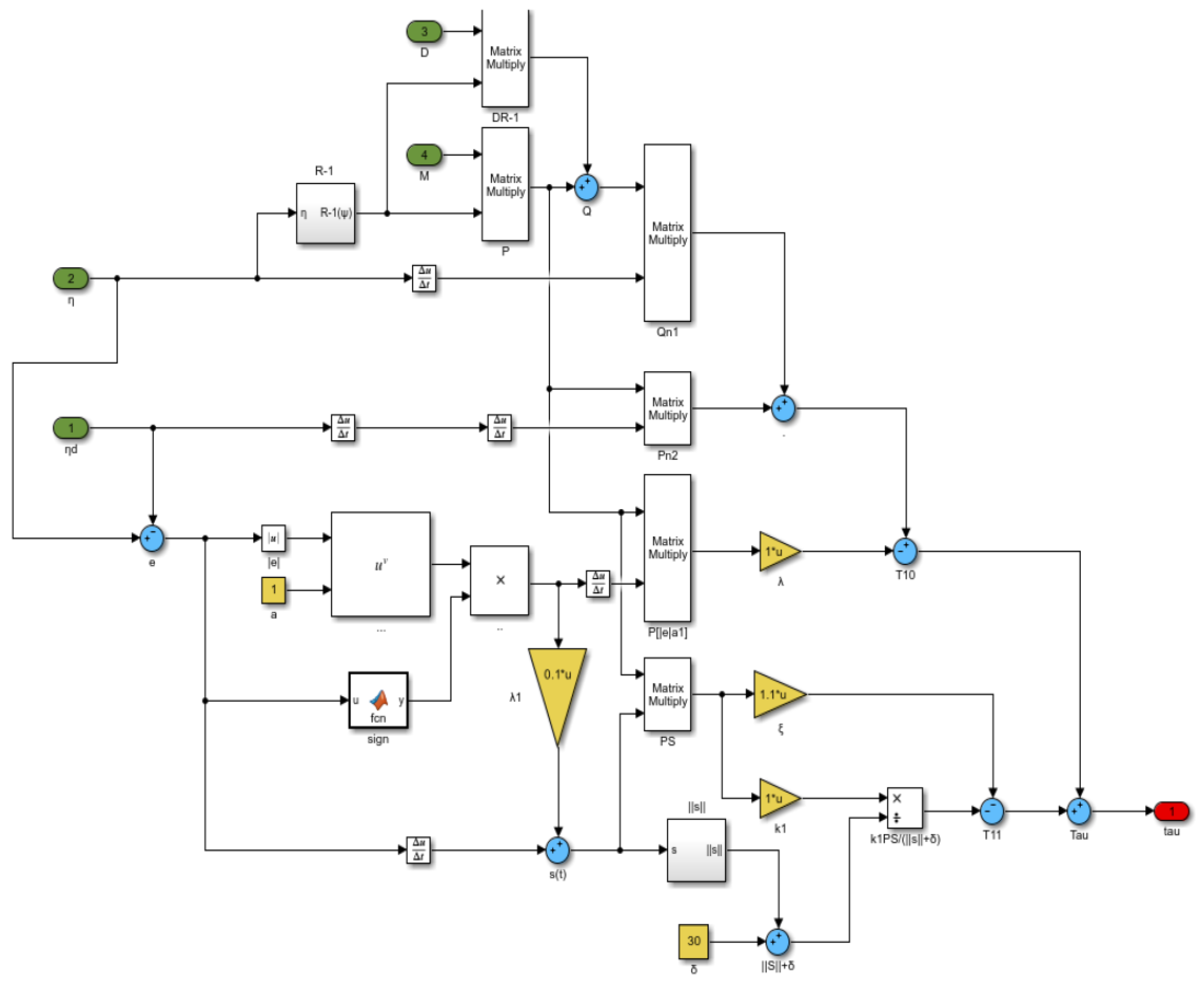
Based on this control law, the controller model is designed as follows Figure 1, the dots (.. …) means that there is no name or the name is already indicated in the box. u indicates the set parameter value [8]:
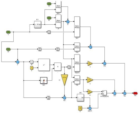
Figure 1.
Simulation model of terminal sliding mode controller for ship dynamic positioning.
4. Crayfish Optimization Algorithm
Algorithmic Principle
The Crayfish Optimization Algorithm (COA), introduced in 2023, is a metaheuristic optimization algorithm inspired by the behaviors of crayfish, including their cooling, competition, and foraging activities. These behaviors correspond to the algorithm’s cooling phase, competition phase, and foraging phase, respectively. The competition and foraging phases are the development stages of the COA, while the cooling phase represents the exploration stage of the algorithm [11]. The Crayfish Optimization Algorithm is a newly emerging algorithm in recent years. We conducted a comprehensive comparison test of this algorithm alongside other traditional optimization methods. These tests included evaluating the performance of each algorithm on multiple benchmark functions to compare their optimization accuracy, convergence speed, and stability. Specifically, we measured the algorithms’ ability and efficiency in handling different optimization problems, including how they deal with complex search spaces and un-certainties. Through these systematic comparisons, we found that the Crayfish Optimization Algorithm outperforms other methods in terms of accuracy, convergence, and robustness, especially in effectively finding global optima for complex optimization problems. However, there are still some limitations, so we adopted multiple strategies to optimize the crayfish algorithm in order to achieve better optimization performance.
The development and exploration of the COA rely on temperature regulation, with temperature acting as a random variable. When the temperature is too high, crayfish seek out caves for cooling. If no other crayfish are in the cave, they will enter directly, which corresponds to the cooling phase of the algorithm. If other crayfish are present in the cave, competition ensues, indicating that the algorithm is in the competition phase. When the temperature is moderate, the algorithm enters the foraging phase. In the foraging phase, crayfish decide whether to consume food directly or shred it before eating, depending on the size of the food. Through improvements in temperature balancing, the Crayfish Optimization Algorithm can more efficiently find the optimal fitness value.
Initialization: In multi-dimensional optimization problems, each crayfish corresponds to a 1× dim matrix, where each column represents a solution. The COA algorithm initializes by randomly generating N candidate solutions X between the lower and upper bounds, where N denotes the population size and dim denotes the problem dimension. The initialization step is as follows:
In the above formula, denotes the lower bound of the j-th dimension, denotes the upper bound of the j-th dimension, and rand is a random number in the range [0, 1].
Defining Temperature and Crayfish Foraging Amount: Temperature variations affect crayfish behavior, causing them to enter different stages. The temperature is defined as shown in Equation (3). When the temperature exceeds 30 °C, crayfish seek cool places to avoid heat; at suitable temperatures, they begin foraging. The foraging amount of crayfish is influenced by temperature, with the optimal range being between 15 °C and 30 °C, and 25 °C being the best. Therefore, the crayfish’s foraging amount can be approximated by a normal distribution, reflecting the impact of temperature. The mathematical model for crayfish foraging amount and the corresponding amounts at different temperatures are shown in the following formula.
Here, temp denotes the temperature of the environment where the crayfish are located.
Here, μ denotes the optimal temperature for the crayfish, while and are used to control the crayfish’s intake at different temperatures.
Cooling Stage: When the temperature exceeds 30 °C, it indicates that the temperature is too high. At this point, crayfish will seek out caves to cool down. The definition of the cave is as follows:
Here, denotes the optimal position obtained through the number of iterations, and denotes the optimal position obtained after updating the population of the previous generation.
The competition for caves among crayfish is a random event. In COA, when rand <0.5, this means no other crayfish are competing for the cave, so the crayfish will directly enter the cave to cool down. The formula for crayfish entering the cave is as follows:
Here, t denotes the current iteration number, t + 1 denotes the next iteration number, and is a decreasing curve defined as follows:
Here, T denotes the maximum number of iterations.
Competition Stage: When the temperature exceeds 30 °C and rand ≥ 0.5, this means that other crayfish have also chosen the same cave. At this point, they will compete for the cave. They compete for the cave using the following formula:
Here, z denotes a random individual of the crayfish.
Foraging Stage: When the temperature is less than or equal to 30 °C, it is suitable for crayfish to forage. At this point, crayfish will start searching for food. During foraging, they will decide whether to tear the food based on its size. If the food size is appropriate, the crayfish will consume it directly; if the food is too large, the crayfish will use their pincers to tear it apart and then use their second and third walking legs to alternately grasp and consume the food. The definition of the food is as follows:
The definition of food size is as follows:
Here, is the food factor representing the maximum food size, with a constant value of 3. represents the fitness value of the i-th crayfish, and represents the fitness value at the food’s location.
When , it indicates that the food is too large. At this point, the crayfish will use the following formula to tear apart the food.
After tearing apart the food, the crayfish will use their second and third walking legs alternately to grasp and consume the food. To simulate this alternating feeding behavior, a combination of sine and cosine functions is used to model the alternating process, as shown in the figure. Moreover, the amount of food obtained by the crayfish is also related to the food intake quantity. The feeding equation is as follows:
When , the crayfish will move directly towards the food and consume it. The equation is as follows:
5. Improvement Scheme for the Crayfish Algorithm
5.1. Introduction to Strategy
5.1.1. Principles of the Subtraction Averaging Algorithm
The Subtraction Averaging Algorithm is a technique for optimizing system performance by iteratively adjusting parameters. Its main goal is to improve convergence speed and result accuracy during optimization. The operation process of the algorithm can be divided into the following steps:
- Initialization: Define a set of initial parameter values based on preliminary estimates or experience.
- Difference Calculation: In each iteration, calculate the difference between the current parameter values and the target values. These target values are usually theoretically optimal values or reference values set by external standards.
- Adjustment: Based on the calculated difference, subtract a proportional amount of the difference from the current parameter values. This proportion is typically a pre-set factor used to control the adjustment magnitude. The subtraction operation moves the parameter values towards the target values.
- Averaging: Perform averaging on the adjusted values to reduce the sharp fluctuations that may result from single adjustments. By averaging multiple adjusted values, the adjustment process becomes smoother and reduces instability caused by excessive single adjustments.
- Iteration: Repeat the above steps—difference calculation, adjustment, and averaging—until the parameter values converge to the desired precision level or meet stopping criteria. Stopping criteria may include reaching the maximum number of iterations or the change magnitude falling below a certain threshold.
The advantages of the Subtraction Averaging Algorithm lie in its simplicity and efficiency. By gradually reducing differences and smoothing adjustments, it effectively improves parameter stability and accuracy, minimizing fluctuations during the convergence process. It is applicable in various fields, including control system design, machine learning model optimization, and data smoothing, making it suitable for scenarios requiring precise adjustment and optimization.
5.1.2. Levy Flight
Levy Flight is a stochastic process used for optimization and search, characterized by a combination of long and short jumps to effectively explore the global search space. This method mimics the foraging behavior of certain animals in nature, such as bees and seagulls, which exhibit specific jump patterns while searching for food. The core principles are:
Core Principle: The key feature of Levy Flight is that its step lengths follow a Levy distribution, which has heavy tails, allowing occasional long-distance jumps. These long jumps help the algorithm explore globally, effectively avoiding local optima. Short jumps assist in fine-tuning within local areas, improving local optimization.
Main Characteristics:
Long Jump Capability: Levy Flight allows for occasional long-distance jumps, helping to escape local optima and enhance global search capabilities.
Short Jump Capability: Short jumps help in fine-tuning and optimizing within local regions.
Heavy-Tailed Distribution: The Levy distribution of step lengths means that while long jumps are rare, they are possible, providing effective exploration of the global space.
Levy Flight is widely used in optimization algorithms, path planning, and data analysis. It enhances the global search capability of algorithms such as Particle Swarm Optimization (PSO) and Ant Colony Optimization (ACO), improves optimization efficiency, and provides effective search strategies in large-scale datasets and complex data distributions.
5.1.3. Sparrow Search Algorithm
The Magpie Search Algorithm (SSA) is a swarm intelligence optimization algorithm inspired by the collaborative behavior and information exchange of magpies during foraging. It simulates the roles of producers and consumers within a magpie flock and their collaborative behavior to find optimal solutions to problems. In a magpie flock, there are two roles: discoverers who search for food and provide information about foraging areas, and joiners who use the information from discoverers to obtain food. This simulation reflects the natural state of mutual monitoring among individuals, where joiners compete for food resources to improve their own foraging efficiency. All individuals remain vigilant to avoid predators during foraging.
- Abstracted Biological Characteristics:
- Producers: High-energy magpies that provide information about foraging areas and evaluate food sources based on individual health values.
- Alarm Signals: When magpies detect predators, they start calling out as an alarm signal. If the alarm level exceeds a safety threshold, producers guide all joiners to a safe area.
- Role Transition: Any magpie searching for better food sources can become a producer, but the ratio of producers to joiners remains constant within the population.
- Energy Levels: High-energy magpies act as producers, while hungry joiners may fly to other areas in search of more energy.
- Foraging Behavior: Joiners follow producers to find food, and some joiners may monitor producers to compete for food and improve their own foraging efficiency.
- Safety Behavior: Magpies on the edge of the flock move quickly to a safe area upon detecting danger, while those in the center move randomly to stay close to other magpies.
- Algorithm Steps:
- Initialization: Randomly generate a group of magpie individuals, each representing a potential solution, and initialize the positions of scouting and foraging magpies.
- Scouting Magpies Search: Scouting magpies perform random walks in the search space to discover new food sources (candidate optimal solutions).
- Foraging Magpies Search: Foraging magpies perform local searches around the food sources discovered by scouting magpies to find better solutions.
- Position Update: Update the positions of magpie individuals based on the search results of scouting and foraging magpies and update the global best solution.
- Iteration: Repeat the scouting and foraging processes until stopping conditions are met (such as reaching the maximum number of iterations or achieving the desired optimization precision).
5.2. Algorithm Improvement
5.2.1. Subtraction Averaging Algorithm
In the competitive phase of the crayfish algorithm, the Subtraction Averaging Algorithm is introduced with a 0.5 probability to select which method to use for competition. The algorithm dynamically adjusts individual positions, using the differences between the current solution and other solutions to effectively enhance local search capability. This adjustment not only helps the algorithm to explore the vicinity of the current solution more thoroughly but also improves solution quality by reducing ineffective searches, thus increasing the precision of the final solution. The Subtraction Averaging Algorithm also enhances the diversity of the population, preventing the algorithm from getting trapped in local optima, and balancing exploration with exploitation. Additionally, this method improves the stability of the algorithm, making the search process smoother and more consistent. Therefore, the introduction of the Subtraction Averaging Algorithm enhances the Crayfish Optimization Algorithm’s global search capability and performance in solving complex optimization problems.
Difference Calculation:
Here, represents the difference value from the previous dimension, and is the adjustment term for the current dimension. The term indicates the sign of the fitness difference, used to adjust the direction.
New Position Calculation:
Here, represents the scaled difference value based on a random number. The term adjusts the position of the current individual by scaling the difference value. is the optimal solution position in the d-th dimension, used to update the position.
5.2.2. Levy Flight Strategy
Introducing the Levy Flight Strategy perturbs the current position during the foraging phase with a 0.5 probability, balancing the original algorithm’s operations with Levy mutations. This integration significantly enhances the algorithm’s global search capability and optimization performance. Levy Flight introduces random perturbations with long jumps, enabling broader exploration of the solution space and helping the algorithm escape local optima to discover better global solutions. This strategy effectively improves search efficiency, particularly in complex and high-dimensional optimization problems, reducing convergence time and improving solution quality. Additionally, Levy Flight increases population diversity, preventing the algorithm from getting trapped in local optima, and maintains a good balance between exploring new solutions and local exploitation. This makes the optimization process more comprehensive and efficient, ultimately enhancing the overall performance of the algorithm [12]
- Levy Flight Factor Selection:Here, represents a perturbation factor vector based on the Levy distribution, and is a vector of ones with dimension dim.
- Handling Small Food SizesWhen the food size is too small, the crayfish moves directly towards the food and consumes it. The original algorithm’s Formula 5 is updated as follows:
- Handling Large Food Sizes : when the food size is too large, the crayfish feeding Formula 6 is updated as follows:
5.2.3. Sparrow Search Position Update Strategy
Drawing on the ideas from the Sparrow Search Algorithm, an improved position update formula is introduced, which is crucial for enhancing global search and development capabilities. This improvement increases the likelihood of escaping local extrema, making the overall optimization functionality of the algorithm more outstanding. The Sparrow Search Strategy, by incorporating an exponential decay factor in position updates, aids the algorithm in escaping local optima and increases the chances of exploring new regions, thereby improving the probability of finding the global optimum. Additionally, this strategy enhances the algorithm’s diversity and robustness, allowing it to dynamically adjust its search behavior according to the optimization phase, thereby improving optimization efficiency and effectiveness [13].
- Judgment Formula:rand < STFirst, generate a random number ‘rand’. If this random number is less than the threshold ST, then apply the Sparrow Search Position Update Strategy.
- Update Formula:
Here, Factor is the exponential decay factor, which decreases gradually with the increase in the number of iterations. The value of Factor is influenced by the random number and the maximum number of iterations. The calculation formula for Factor is as follows:
where current iteration is the current iteration count, serving as an indicator of the iteration progress. The random number variable is a random number within the range [0, 1], and total iterations is the total number of iterations. As the number of iterations increases, the value of Factor gradually decreases. This helps to reduce the magnitude of position updates in the later stages of iteration, making updates more subtle and maintaining stability in the search process during the optimization’s later phases.
5.3. Algorithm Flow
The algorithm flow of parameter optimization of terminal sliding film controller based on JLSCOA is given below:
- Initialize the algorithm parameters: set the number of iterations T, the number of populations, the number of variables dim, and the upper and lower boundaries L and H. Initialize the population position X, calculate the initial fitness value, and determine the initial global optimal solution and the best fitness.
- Enter the main loop: the number of iterations starts from 1 until T is reached.
- Update temperature and learning factor: in each iteration, randomly generate the temperature temp and update the learning factor C according to the current iteration number.
- Calculate food location: calculate food location based on the current optimal solution.
- Population position update:If temperature temp > 30, enter the heat avoidance phase:randomly choose a probability of 0.5 to update the location.If not entering the heat avoidance phase, choose with probability 0.5 to enter the competitive phase or the improved subtractive averaging algorithm strategy.If temperature temp ≤ 30, enter the foraging phase:introduce a Levy Flight strategy to perturb the current position, selecting with probability 0.5 to use.Calculate p-value and adjust population position by determining food size based on p-value.
- Introduction of sparrow search strategy: introduce the position update strategy of sparrow search for some individuals to enhance the global exploration ability.
- Boundary processing: ensure that the updated population position is within the upper and lower boundaries.
- Fitness value update: calculate the fitness value of the updated population and update the global optimal solution and the current optimal solution.
- Record the current optimal solution and fitness value: record the global optimal solution and fitness value of the current iteration.
- Check the termination condition: if the iteration number reaches the maximum, output the optimal solution, otherwise continue iteration.
6. Algorithm Performance Testing
6.1. Algorithm Performance Testing Numerical Experiments
In order to verify that the stability and optimization effect of the improved crayfish algorithm is stronger than other algorithms, this paper uses the commonly used 12 algorithmic test functions to test and compare the algorithmic test functions and the information in Table 2. Six uni-modal and six multi-modal benchmark functions were used to evaluate the performance of JLSCOA. These functions were chosen to cover a range of optimization scenarios, including both uni-modal and multi-modal features. Uni-modal functions are very effective for evaluating the accuracy and convergence behavior of the algorithm, while multi-modal functions challenge the algorithm’s ability to perform global search and avoid local optima. This combination ensures a robust evaluation of JLSCOA’s capabilities.
Table 2.
Benchmark function.
6.1.1. Algorithm Parameterization and Evaluation Metrics
In view of the fairness of the comparison test, all four algorithms were set with the same common parameters as follows:
For continuous single-peak functions, the local optimum is the global optimum, which is often used to test the convergence speed and convergence accuracy of the algorithms; multi-peak functions have multiple local optima, which can assess the ability of the algorithms to jump out of the local optimum and find the global optimum. In order to reduce the error caused by the randomness of the algorithms, for each test function, the four algorithms are independently performed 30 times, the optimal value and the worst value of each function in each group of results are recorded, and the average and standard deviation of the results of the 30 operations are obtained, which are used as the evaluation indexes of the algorithms’ performance. The optimal value and the worst value reflect the quality of understanding, the average value reflects the accuracy that the algorithm can achieve, and the standard deviation reflects the robustness and stability of the algorithm [4].
6.1.2. Comparative Analysis with Other Intelligent Algorithms
Simulation comparison test of COA, WOA, SSA, and JLSCOA in Matlab R2024a, Table 3 is a comparison of the best value, worst value, average value, and standard deviation of the four algorithms after solving the uni-modal benchmark function. Table 4 is a comparison of the best value, worst value, average value, and standard deviation of the four algorithms after solving the multi-modal benchmark function.4 algorithms performance test numerical test comparison results are shown in Table 4 and Table 5.
Table 3.
Values of public parameters for algorithm comparison tests.
Table 4.
Comparison of the performance of four algorithms, such as COA, JLSCOA, WOA, and SSA, for solving single-peak benchmark tests.
Table 5.
Comparison of the performance of four algorithms, such as COA, JLSCOA, WOA, and SSA, for solving multi-peak benchmark tests.
In the six single-peak benchmark functions, JLSCOA and COA find the theoretical optimum of 0, the mean of the worst values, and the standard deviation of 0 in solving f1, f2, f3, and f4. The other two algorithms tend to fall into the local optimum in solving f4 and thus do not arrive at the theoretical optimum. In solving f5 and f6, JLSCOA is not as good as the other two algorithms, but it is significantly better than COA. In the six multi-peak benchmark functions, JLSCOA outperforms the other algorithms in solving f7, f8, f9, f10, and it is at least two orders of magnitude better than SSA and WOA, and JLSCOA is not as good as the other two algorithms in solving f11 and f12, but is significantly better than COA. In summary, compared with WOA and SSA, JLSCOA has a big advantage over COA, and its performance in different functions is basically ahead of COA in all aspects, and compared with the other algorithms, JLSCOA has 83% of the advantage in finding the optimal value, 83% of the advantage in finding the average value, and 75% of the advantage in finding the standard deviation, and it has a stronger robustness. It is proven that the multi-strategy improved JLSCOA based on the basic COA has effectiveness and superiority and is a more efficient algorithm.
7. Parameter Optimization of Terminal Sliding Film Controller Based on JLSCOA
7.1. Fitness Function
In this paper, we take the terminal sliding film controller of the power positioning system based on the “New Hongzhu” ship of Dalian Maritime University as the research object, and search for the optimal values of two parameters that have a big influence on the control results: the parameter δ used to eliminate the jitter vibration, and the control gain λ on the surface of the sliding mode, and design the adaptivity function as follows:
where the coefficients c and b are the weights of the system error and the control quantity, respectively, representing the importance of the energy consumption requirement and the error tracking requirement [14].
7.2. Simulation Experiment and Result Analysis
7.2.1. Simulation Experiment Parameters
The initial position of the ship is set as [0 m, 0 m, 0°], and the desired position is set as [5 m, 5 m, 10°], and the simulation time is 600 s. The parameters to be optimized are set as λ and δ; the initial population size N = 6, the lower bound of the initial solution L = [1, 1], and the upper bound of the initial solution H = [500, 500], and the number of iterations is T = 30. The other parameters of the controller are set as . The weighting factor of the fitness function is set as c = 0.15, b = 0.1.
7.2.2. Simulation Experiment Results
First, the controller parameters are optimized and simulated using COA and JLSCOA, respectively. The simulation results are shown in Figures 3 and 4. The optimized controller parameters as well as the fitness function values are shown in Table 6.
Table 6.
Optimized controller parameter results and fitness values.
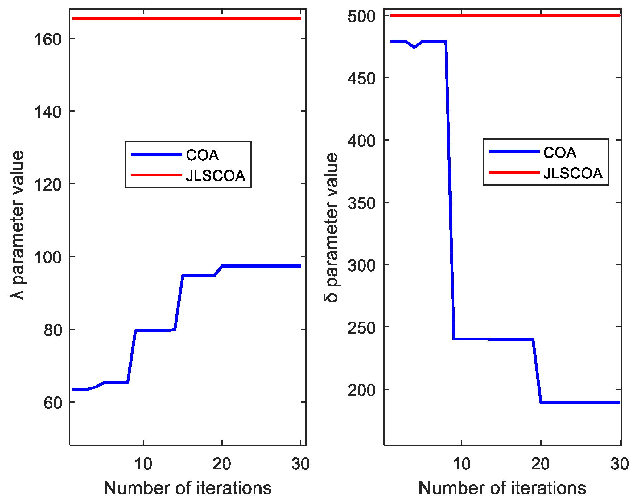
Based on Figure 2 and Figure 3, it can be seen that after the second generation of iterations, the JLSCOA algorithm quickly finds the global optimum, and the parameters of the controller reach their optimal values. Additionally, JLSCOA demonstrates greater stability during the iteration process, resulting in a smaller final fitness value. This highlights the superior performance of JLSCOA compared to the traditional crayfish algorithm in optimizing the parameters of the terminal sliding mode controller.

Figure 2.
Parameters λ and δ iterative variation curves.
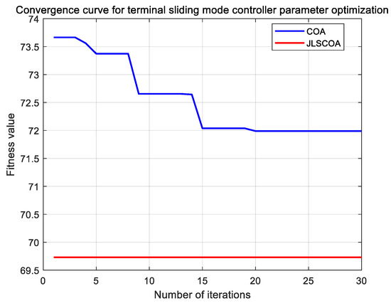
Figure 3.
Fitness function iteration variation curve.
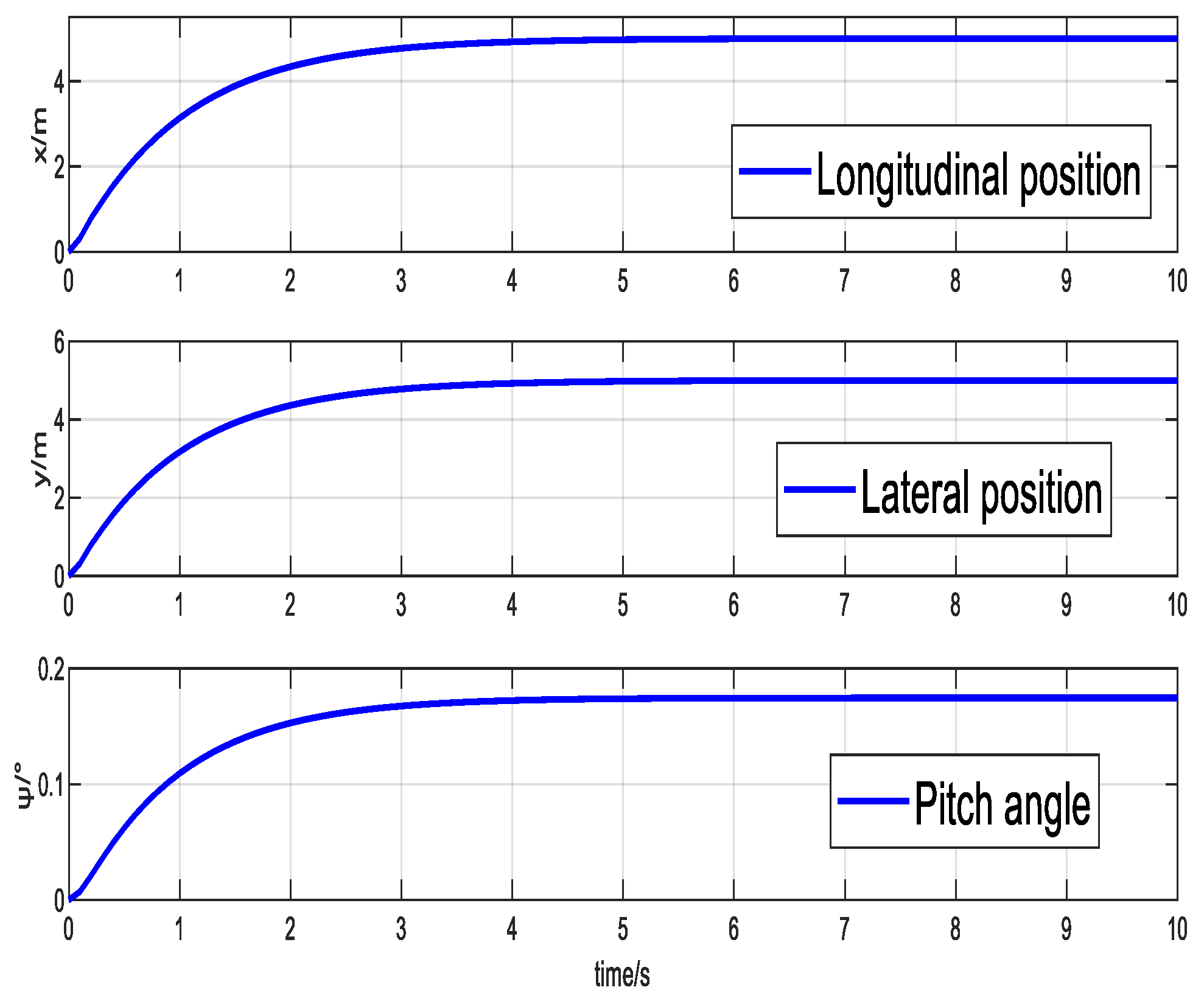
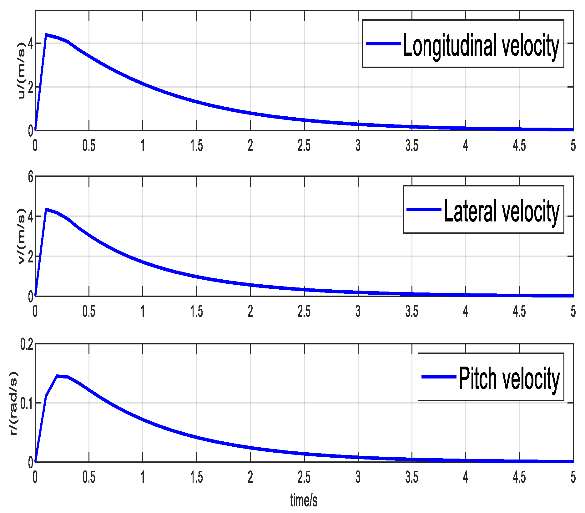
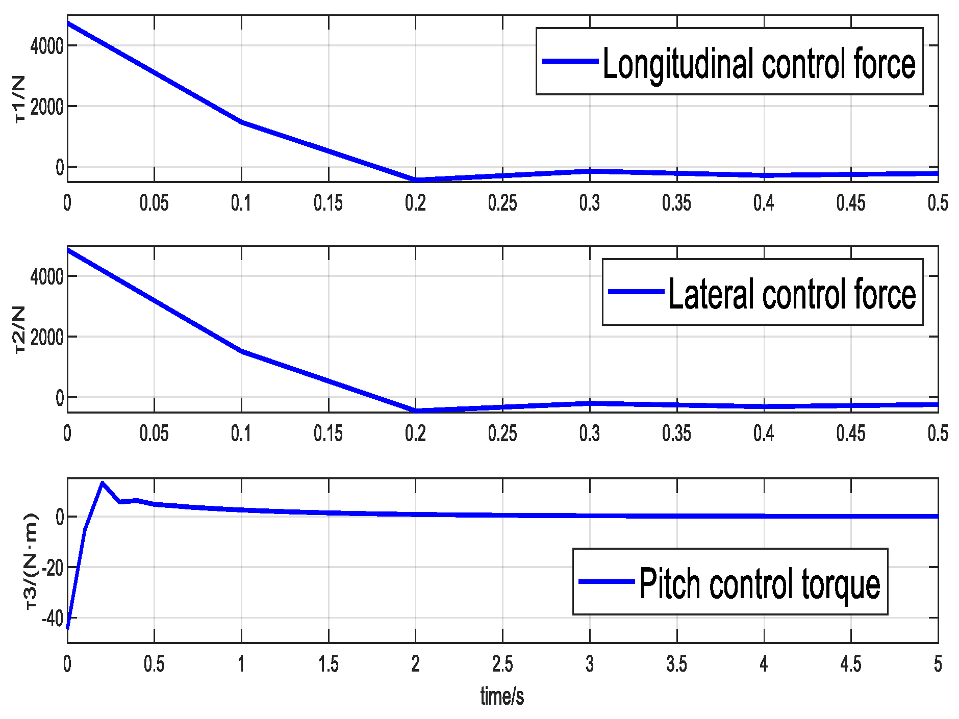
Using the “Xin Hongzhuan” ship from Dalian Maritime University as the simulation object, performance verification of the terminal sliding mode controller optimized by JLSCOA is conducted in an ideal environment. The initial position of the ship is set to [0 m, 0 m, 0°], and the desired position is set to [5 m, 5 m, 10°]. Other controller parameters are set as . The simulation time is 600 s. Figure 4, Figure 5 and Figure 6 show the results. Figure 4, Figure 5 and Figure 6 are the curves of the change of position, speed, and control force of the ship’s three freedoms.
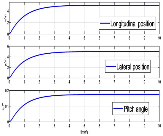
Figure 4.
Ship position and pitch angle variation curve.
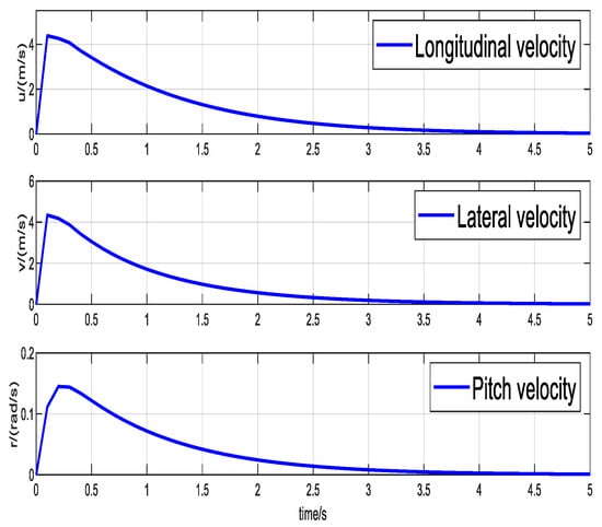
Figure 5.
Ship velocity variation curve.
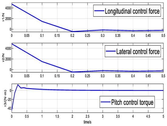
Figure 6.
Ship control force curve.
From Figure 4, it can be seen that under the control of the terminal sliding mode controller optimized by JLSCOA, the ship can stabilize at the desired position [5 m, 5 m, 10°] from the initial position [0 m, 0 m, 0°] within a limited time. The positioning process is stable, and the response time is quick. Figure 5 shows that the sliding mode control force output is continuous and bounded, with both the magnitude and process of the control force being within a reasonable range. Figure 6 indicates that the ship’s velocity changes smoothly from zero to a larger value and then back to zero, demonstrating that the entire positioning process is relatively stable. This suggests that the system control performance is ideal and meets the accuracy requirements of most practical engineering applications, highlighting the effectiveness of the terminal sliding mode controller optimized by JLSCOA.
A comparative simulation analysis is performed between the terminal sliding mode controller with given parameters and the terminal sliding mode controller optimized using the JLSCOA algorithm. The parameters of the given terminal sliding mode controller are .
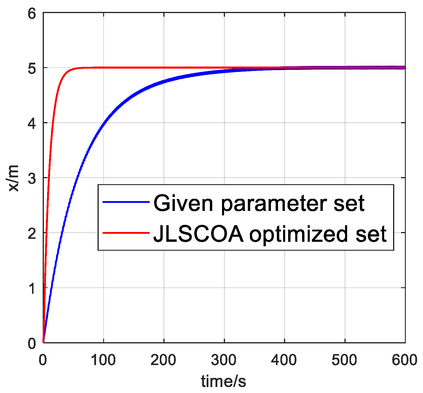
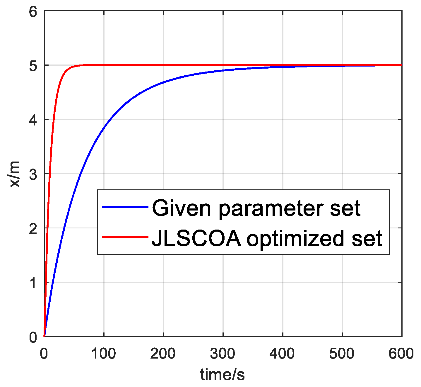
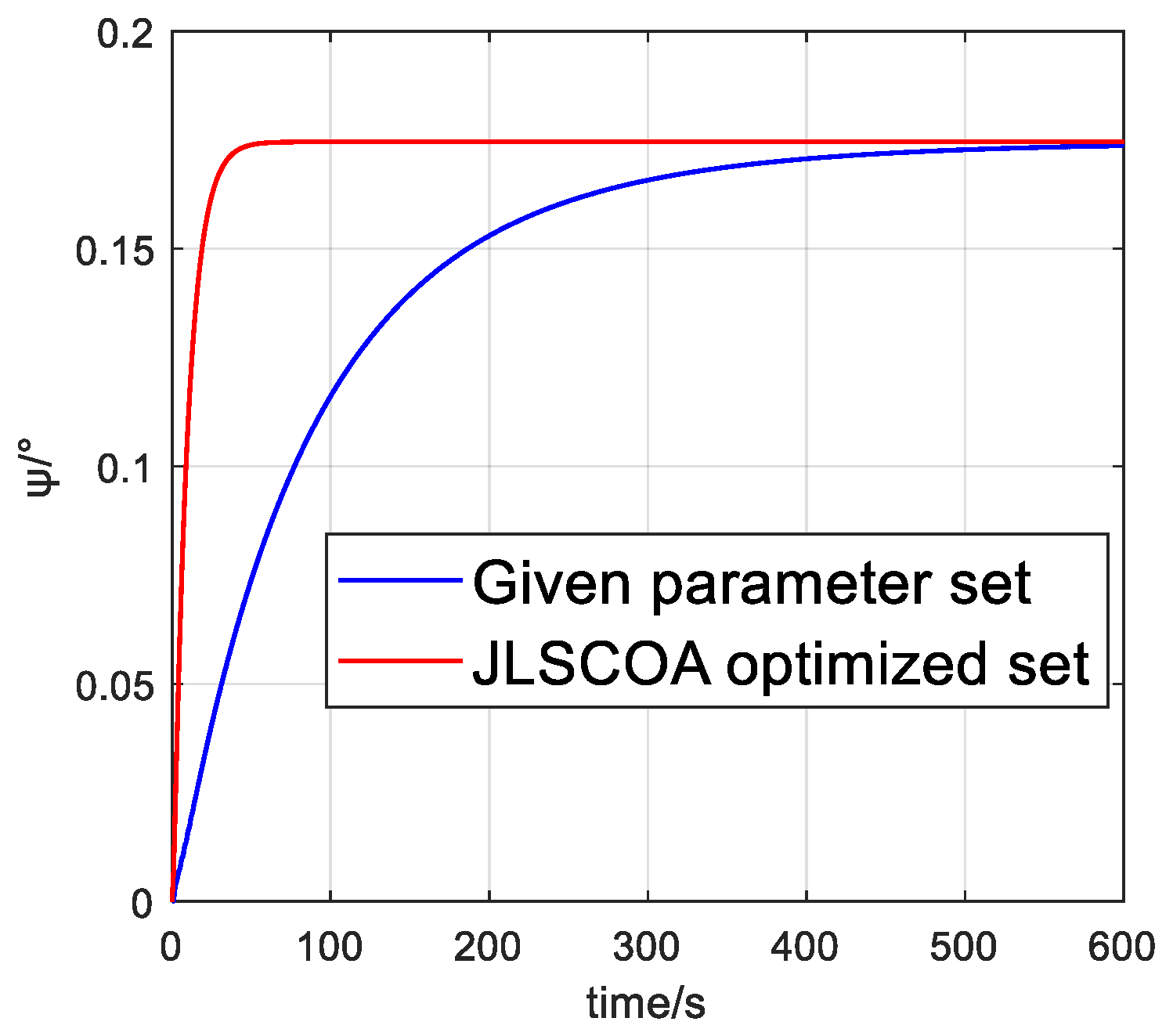
Figure 7, Figure 8 and Figure 9 show the position variations of the ship in three degrees of freedom. From the figures, it can be seen that the ship equipped with the terminal sliding mode controller optimized by the JLSCOA algorithm can complete the positioning process more quickly, with an average position change time of approximately 300 s faster than that of the given parameter set.
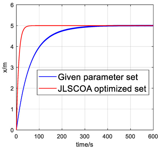
Figure 7.
Comparison of longitudinal position variations.
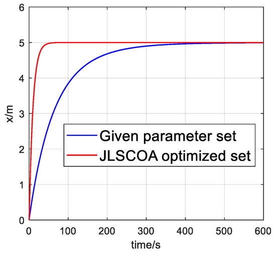
Figure 8.
Comparison of lateral position variations.

Figure 9.
Comparison of pitch angle variations.
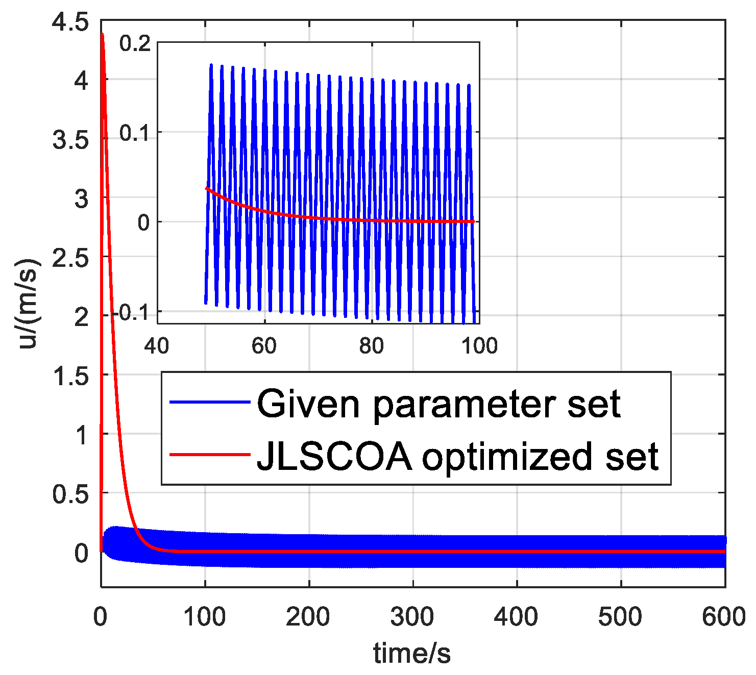
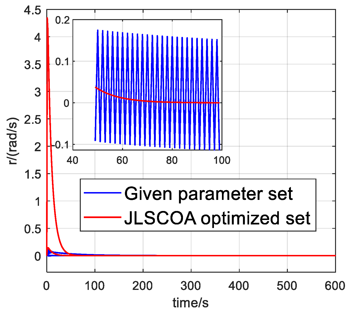
Figure 10, Figure 11 and Figure 12 depict the velocity variations in three degrees of freedom. The results indicate that the given parameter set exhibits significant velocity oscillations and smaller control forces, while the JLSCOA optimized set shows larger control forces with almost no velocity oscillations.
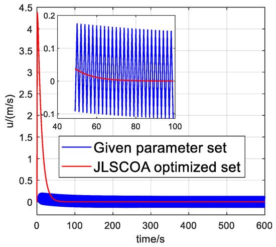
Figure 10.
Comparison of longitudinal velocity variations.
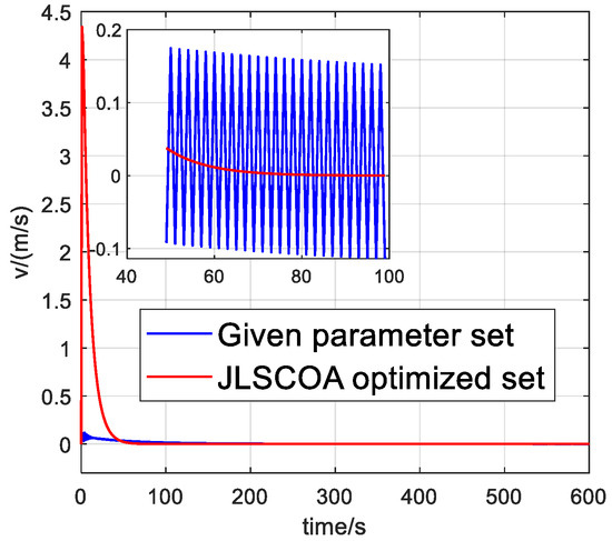
Figure 11.
Comparison of lateral velocity variations.
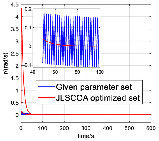
Figure 12.
Comparison of pitch rate variations.
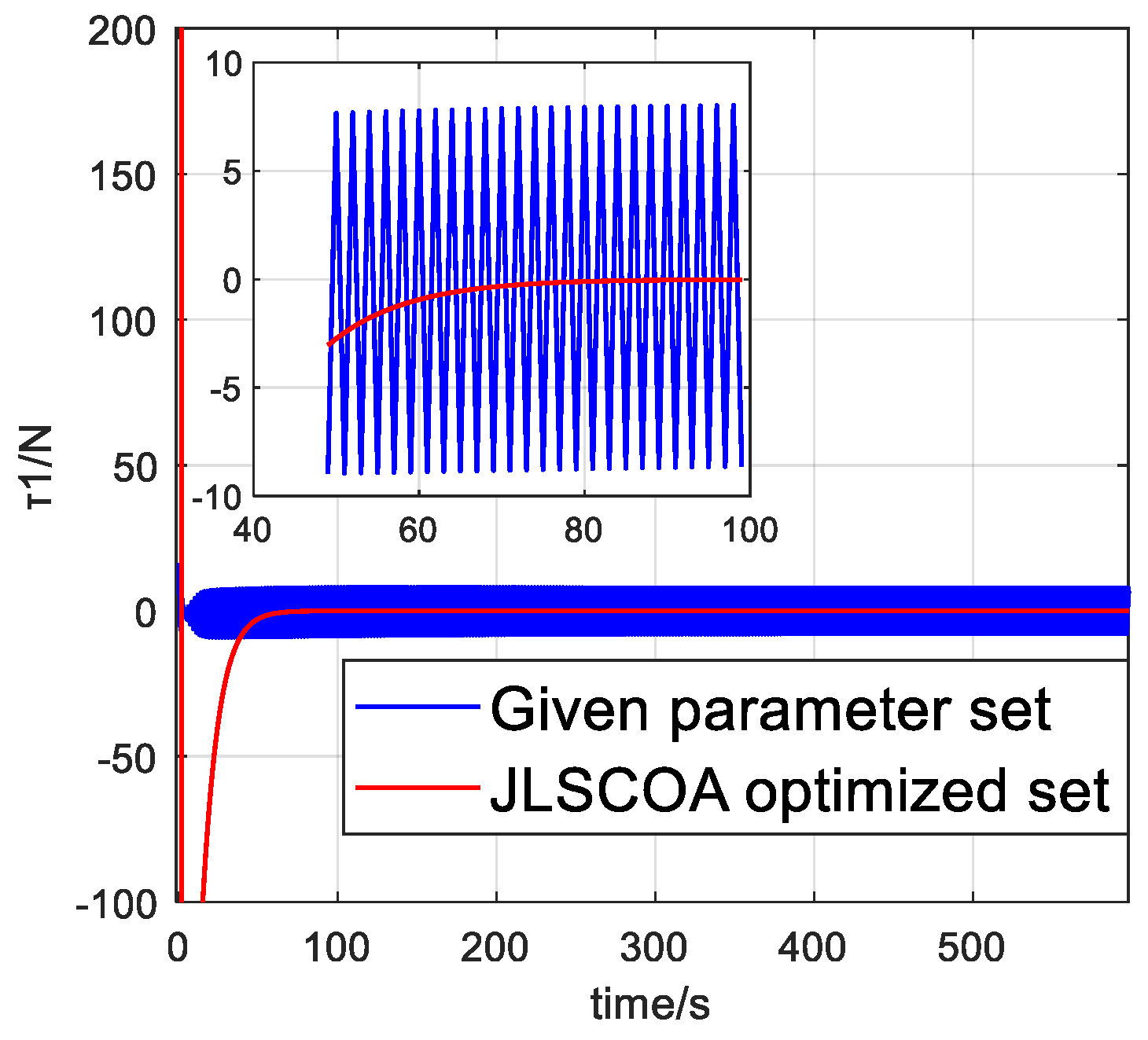
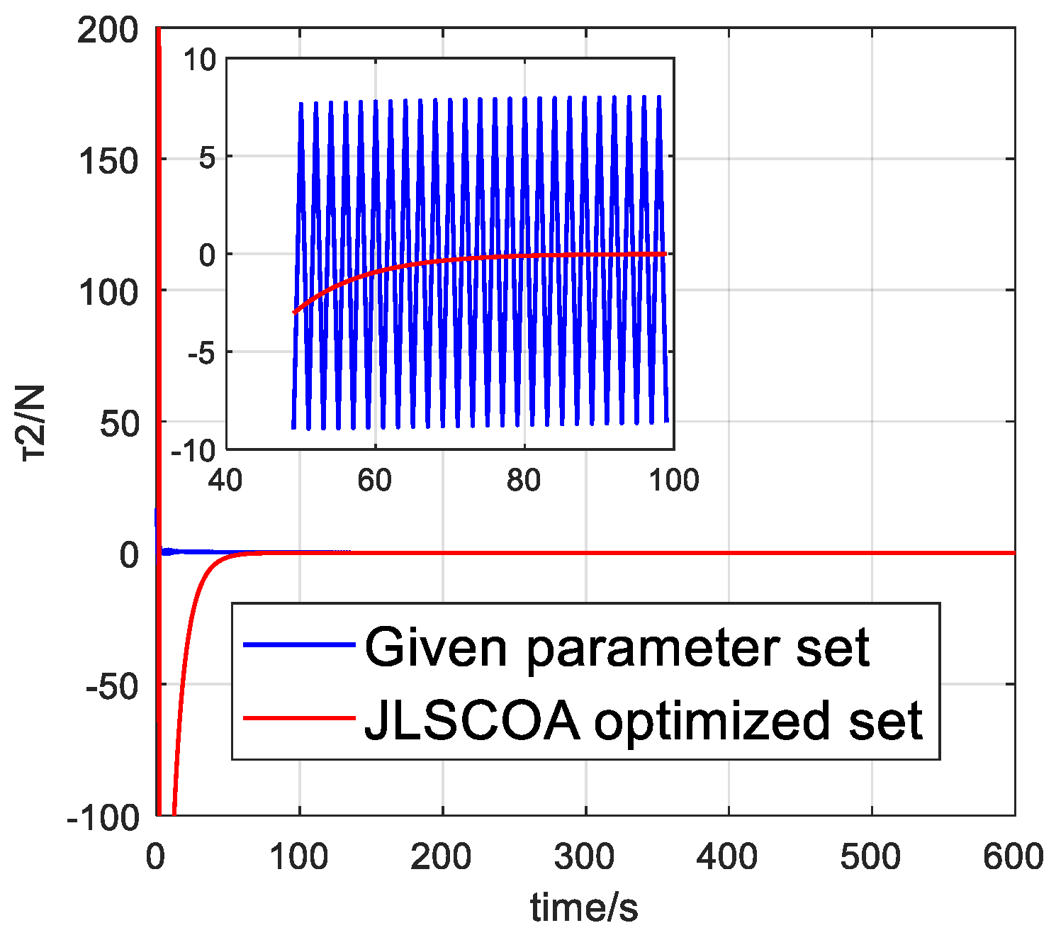
Figure 13, Figure 14 and Figure 15 illustrate the variations in the output force and torque of the terminal sliding mode controller. Analysis reveals that the control force of the given parameter set oscillates significantly, whereas the JLSCOA-optimized set exhibits minimal oscillation.

Figure 13.
Comparison of longitudinal control force variations.

Figure 14.
Comparison of lateral control force variations.
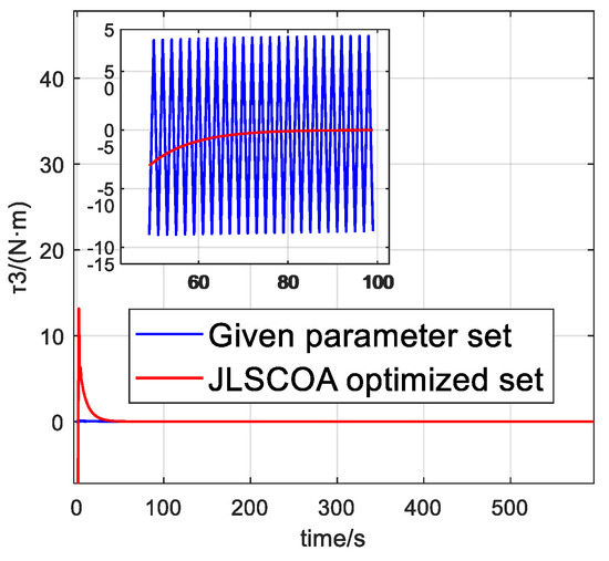
Figure 15.
Comparison of pitch control torque variations.
8. Conclusions
This paper proposes an improved crayfish algorithm based on multi-strategy fusion (JLSCOA) for optimizing the parameters of the terminal sliding mode controller in ship dynamic positioning systems. To address issues with the traditional crayfish algorithm, such as susceptibility to local optima, slow convergence in later iterations, and insufficient optimization accuracy, improvements have been made by incorporating subtraction averaging strategies, Levy Flight strategies, and sparrow search position update strategies.
Comparative tests with COA, WOA, and SSA optimization algorithms show that JLSCOA outperforms the others with an 83% advantage in finding the optimal value, an 83% advantage in average performance, and a 75% advantage in standard deviation, indicating stronger optimization capability and robustness. JLSCOA demonstrates significant advantages in optimization accuracy, convergence performance, and stability.
The application of JLSCOA to optimize the parameters of the terminal sliding mode controller has been verified through simulations on the “Xin Hongzhuan” ship from Dalian Maritime University. The simulation results indicate that the terminal sliding mode controller optimized by JLSCOA significantly outperforms the traditional un-optimized controller in terms of disturbance resistance, response speed, and system stability. The average time for three-degree-of-freedom position changes is over 300 s faster compared to the given parameter set, and control force and velocity oscillations are nearly eliminated. JLSCOA not only enhances the performance of the terminal sliding mode controller but also reduces parameter tuning difficulty, improving the robustness and reliability of the control system. This provides new insights and methods for the design and optimization of practical ship dynamic positioning systems.
In summary, the application of the multi-strategy fusion improved crayfish algorithm in optimizing the parameters of the terminal sliding mode controller for ship dynamic positioning systems shows significant effects, demonstrating its practicality and superiority in complex environments, and providing important reference value for future research and practical applications.
Author Contributions
Conceptualization, Z.W.; Funding acquisition, Z.H.; Investigation, F.Y.; Methodology, Z.W.; Project administration, Z.W.; Software, Z.W.; Validation, B.S.; Writing—original draft, Z.W.; Writing—review and editing, Z.W. All authors have read and agreed to the published version of the manuscript.
Funding
This research was funded by the Innovation Project of the Offshore LNG Equipment Industry Chain: CBG3N21-2-7; the High-technology Ship Research Program: CBG3N21-3-3; and new technology equipment for rapid and green elimination of COVID-19 hydroxyl radicals in cold chain logistics: 62127806.
Institutional Review Board Statement
Not applicable.
Informed Consent Statement
Not applicable.
Data Availability Statement
The data presented in this study are available on request from the corresponding author. The data are not publicly available due to privacy.
Acknowledgments
The authors extend their appreciation to the anonymous reviewers for their valuable feedback.
Conflicts of Interest
The authors declare no conflicts of interest.
References
- Shengyan, H.; Zhongqing, C.; Shengwei, Y. PID Parameter Optimization Based on Flower Pollination Algorithm. Comput. Eng. Appl. 2016, 52, 59–62. Available online: http://cea.ceaj.org/EN/Y2016/V52/I17/59 (accessed on 7 September 2022).
- Lianqiang, Z.; Dongfeng, W. PID Parameter Optimization Based on Improved Crowd Search Algorithm. Comput. Eng. Des. 2016, 37, 3389–3393. [Google Scholar]
- Zifa, L.; Wei, Z.; Zeli, W. Optimization Layout of Urban Electric Vehicle Charging Stations Based on Quantum Particle Swarm Optimization Algorithm. Trans. China Electrotech. Soc. 2012, 32, 39–45. [Google Scholar]
- Tang, Y.Q.; Li, C.H.; Song, Y.F.; Chen, C.; Cao, B. Adaptive mutation sparrow search optimization algorithm. J. Beijing Univ. Aeronaut. Astronaut. 2023, 49, 681–692. [Google Scholar] [CrossRef]
- Hua, F.; Hao, L. Improved Sparrow Search Algorithm with Multi-Strategy Fusion and Its Application. Control. Decis. 2022, 37, 87–96. [Google Scholar] [CrossRef]
- Mao, Q.; Zhang, Q. Improved Sparrow Search Algorithm with Cauchy Mutation and Reverse Learning. Comput. Sci. Explor. 2021, 15, 1155–1164. [Google Scholar] [CrossRef]
- Xiao, Z.; Liu, S. Elite Reverse Golden Sine Whale Optimization Algorithm and Its Engineering Optimization Study. Acta Electron. Sin. 2019, 47, 2177–2186. [Google Scholar] [CrossRef]
- Wei, Z.; He, Z.; Wu, X.; Zhang, Q. Power Positioning System Control Study of “Intelligent Research and Internship Vessel” Based on Terminal Sliding Mode. Appl. Sci. 2024, 14, 808. [Google Scholar] [CrossRef]
- Balchen, J.G.; Jenssen, N.A.; Sælid, S. Dynamic positioning using Kalman filtering and optimal control//IFAC/IFIP. In Proceedings of the Symposium on Automation in Offshore Oil Field Operation, Bergen, Norway, 14–17 June 1976; pp. 183–186. [Google Scholar]
- Lin, J. Research on Ship Power Positioning Control and Thrust Distribution. Master’s Thesis, Dalian Maritime University, Dalian China, 2021. [Google Scholar]
- Jia, H.; Rao, H.; Wen, C.; Mirjalili, S. Crayfish optimization algorithm. Artif. Intell. Rev. 2023, 56, 1919–1979. [Google Scholar] [CrossRef]
- Dehghani, M.; Montazeri, Z.; Trojovská, E.; Trojovský, P. Coati Optimization Algorithm A new bio-inspired metaheuristic algorithm for solving optimization problems. Knowl. Based Syst. 2023, 259, 110011. [Google Scholar] [CrossRef]
- Seyedali, M.; Andrew, L. The Whale Optimization Algorithm. Adv. Eng. Softw. 2016, 95, 51–67. [Google Scholar]
- Guang-chi, X.; Da-Wei, Z.; Kai-Wei, Z.; Jing-hua, G. Multi-agent chaos particle swarm optimization algorithm of thrust allocation for dynamic positioning vessels. In Proceedings of the 2015 34th Chinese Control Conference (CCC 2015), Hangzhou, China, 27–30 July 2015; pp. 2389–2396. [Google Scholar]


Disclaimer/Publisher’s Note: The statements, opinions and data contained in all publications are solely those of the individual author(s) and contributor(s) and not of MDPI and/or the editor(s). MDPI and/or the editor(s) disclaim responsibility for any injury to people or property resulting from any ideas, methods, instructions or products referred to in the content. |
© 2024 by the authors. Licensee MDPI, Basel, Switzerland. This article is an open access article distributed under the terms and conditions of the Creative Commons Attribution (CC BY) license (https://creativecommons.org/licenses/by/4.0/).