Abstract
Tailing storage facilities are very complex structures whose failure generally leads to catastrophic consequences in terms of casualties, serious environmental impacts on local biodiversity, and disruptions in the mineral supply. For this reason, structures at risk must be reinforced or decommissioned. One possible option is its reinforcement with compacted filtered tailings stabilized with binders. Alkali-activated binders provide a more sustainable solution than ordinary Portland cement but require an optimization of the tailing–binder mixture, which, in some cases, can lead to a substantial experimental effort. Statistical models have been used to reduce the number of those experiments, but a rational design methodology is still lacking. This methodology to define the right mixture for a required strength should consider both the mixture components and in situ conditions. In this paper, response surface methods were used to plan and interpret unconfined compression strength test results on an iron tailing stabilized with alkali-activated binders. It was concluded that the fly ash content was the most important parameter, followed by the liquid content and sodium hydroxide concentration. From the obtained results, several statistical models were defined and compared according to the definition of a strength prediction model based on a mixture index parameter. It was interesting to observe that models with the porosity cement index still provide reasonable adjustment even when different tailings’ water contents are considered.
1. Introduction
The increasing number of catastrophic accidents in tailing storage facilities (e.g., tailing dams or dry stacks) highlights the need to reinforce these structures. The use of heavy ground improvement technologies such as Jet Grouting or Dynamic Compaction is not possible in these structures due to the risk of static liquefaction induced by vibrations. The reinforcement of existing tailing deposits at risk or the improvement of dry stacks can be performed by building external structural zones capable of containing the possible liquefaction failure of the unstable material. One possibility is to build those structural zones with cemented filtered tailings, improving stability and avoiding the migration of fine particles to the bottom part of the embankment, where, due to very high overburden stresses, they tend to contract upon shear being very prone to liquefaction [1]. Consoli et al. [2] proposed the use of Portland cement to stabilize dry stacks. However, the use of Portland cement (OPC) in large-scale projects is environmentally criticized, as its production is highly energy-intensive, it requires a significant number of natural aggregates, and it is responsible for a large part of world’s greenhouse gas emissions. Alternative binder research is increasingly moving towards replacing OPC in a significant part of future binder applications [3]. Alkali-activated binders (AABs) can significantly increase the strength and stiffness of stabilized soils not only at the laboratory scale [4,5] but also in large-scale tests [6]. AAB is generated by the reaction of a precursor (e.g., aluminosilicate) with an alkaline solution (activator). Since industrial by-products (such as ashes or slags) can be used as precursors, the binder’s global-warming potential is reduced, and the circular economy is favored [7].
AAB has been used to recycle tailings into several applications [8] not only in cement and mortars [9] but also for more geotechnical problems such as backfill or cover materials [10], road base courses [11], or tailing–binder mixtures for stacking [12]. As highlighted by Manavirapast [13], in the cases where mine tailings exhibit a low level of reactivity to be used as precursors, some pre-treatment methodologies (thermal treatment, mechanical activation, alkaline fusion, etc.) or additional precursors (e.g., ashes, slags, metakaolin, etc.) can be used to enhance alkaline activation. However, the AAB binder optimization can take a significant experimental effort especially when the number of variables is large. To overcome this limitation, Surehali et al. [14] used machine-learning and data-transformation methods to predict the strength of an AAB made with tailings, with fewer experiments.
A generalized application of AAB in soil improvement requires a rational methodology to define mixture dosage depending on the desired performance and in situ conditions. For soils stabilized with OPC, a ratio between porosity and volumetric cement content was developed [15,16] called the porosity cement index. Pereira dos Santos et al. [17] applied this index to gold tailing–AAB mixtures, and Consoli et al. [18] also used this index to compare three types of binders to stabilize iron tailings. However, in these works, there was no development of a binder index capable of adjusting the AAB components to tailings in an in situ water content, as this variable was fixed. This is essential because, in mining operations, the tailings conditions may vary significantly [19].
Statistical models based on the Design of Experiments [20] have been applied to cementitious materials [21], to soil–cement mixtures [22], and to AAB–tailing mixtures [23] to reduce the number of experiments but not with the purpose of obtaining a mixture index that could summarize the contribution of each AAB component (precursor, alkaline activator, tailings, and water).
In this work, response surface methods were used to define a strength prediction model based on a mixture index parameter that could represent the mixture components, since previous works have fixed important variables such as tailings’ in situ water content.
2. Materials and Methods
2.1. Materials
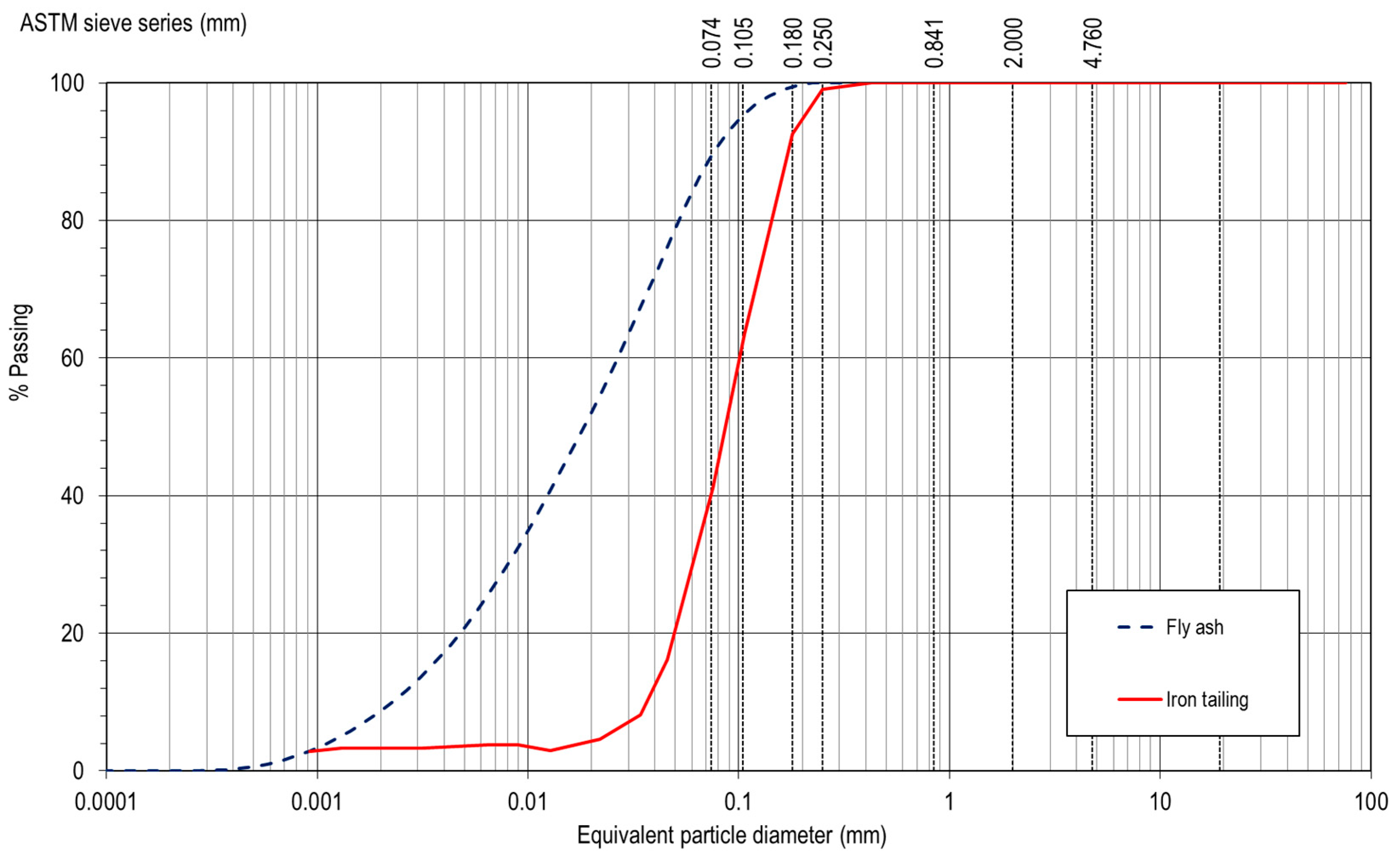
An iron tailing from Minas Gerais, Brazil, classified as a silty sand according to the Unified Classification System [24], was used in this work. The grain size distribution curve is shown in Figure 1, while the main physical parameters are presented in Table 1. The particles unit weight (γS) is quite high (29.5 kN/m3) when compared to natural soils due to the significant iron content.
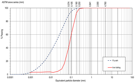
Figure 1.
Iron tailing and fly ash grain size distribution curves.

Table 1.
Iron tailings’ parameters.
The precursor for the alkali activation reactions was a fly ash (FA) classified as type F, according to ASTM standard C 618 [24], due to its low calcium content. Its grain size distribution curve is also shown in Figure 1 for comparison purposes.
The alkaline activator is often made via the combination of sodium hydroxide (SH) and sodium silicate. However, in this work, only SH was used to reduce the carbon footprint. An SH solution of 32% NaOH and 68% water was used, corresponding to a concentration of 11.76 mol/kg, which was diluted for lower concentrations.
Scanning Electron Microscope (SEM) analyses and X-Ray Diffraction (XRD) analyses were performed on both the iron tailings and the fly ash for microstructural characterization of the starting materials.
SEM analyses were performed on a Quanta 400 FEG ESEM (15 kV), made by the FEI company. In this case, the analyses were performed with backscattered electrons detected (BSED) in Z cont mode. This mode is designed to capture backscattered electrons that are reflected on the sample surface. Information about the different components of the sample is obtained according to the intensity of the colors that appear in the images, and the intensity is directly related to the atomic number (Z). When the incident electron beam interacts with the sample, high-Z elements scatter more electrons back towards the detector than low-Z elements. This results in a contrast in the BSE image, with high-Z regions appearing brighter and low-Z regions appearing darker. This contrast allows for the identification of different phases, inclusions, or compositional variations within the sample.
This equipment is equipped with an Energy Dispersive Spectroscopy (EDS) analysis system from the company EDAX with a “Genesis X4M” spectrometer, allowing us to obtain the chemical identification of the components present in the sample.
XRD analyses were performed, at room temperature, by a PANalytical X’Pert Pro diffractometer, equipped with X’Celerator detector and secondary monochromator in θ/2θ Bragg–Brentano geometry. The measurements were carried out using 40 kV and 30 mA, a CuKα radiation (λα1 = 1.54060 Å and λα2 = 1.54443 Å), 0.017°/step, 100 s/step, in a 6–100° 2θ angular range. The diffractograms were interpreted, and the obtained phases were identified and quantified using the software HighScore Plus 4.8. Before performing the analysis, the samples were grinded and then assembled in a standard sample holder for powders.
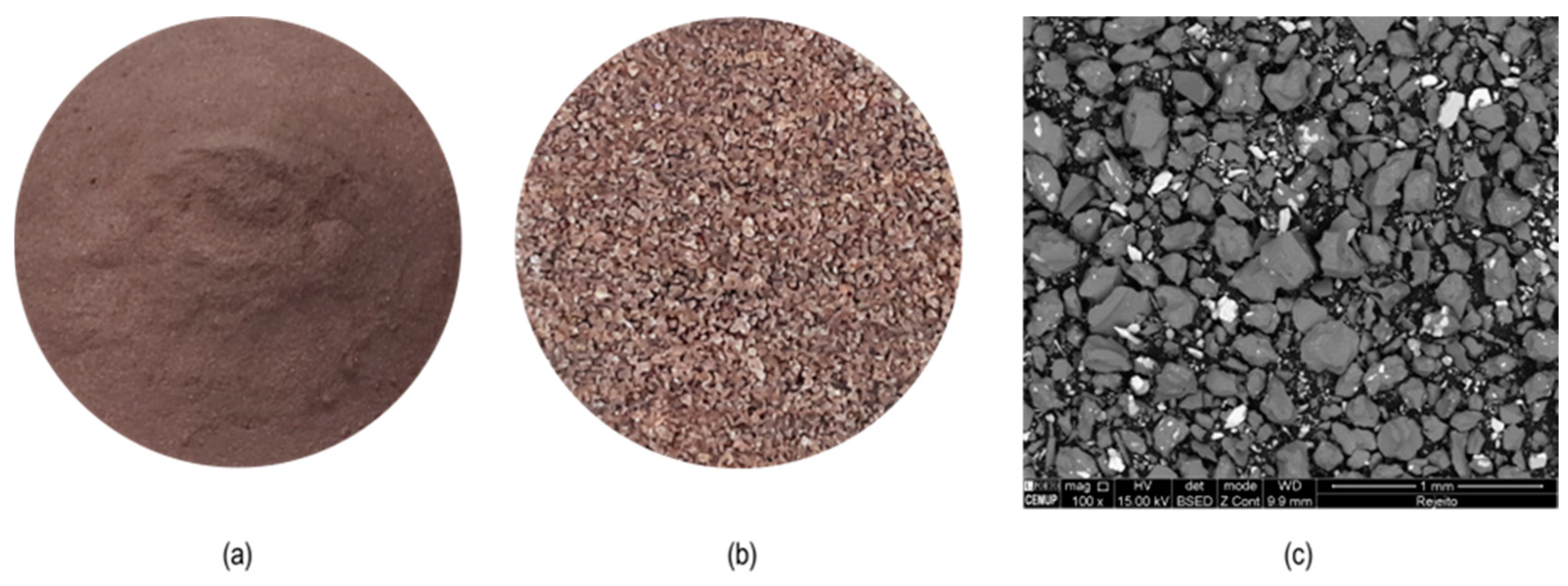
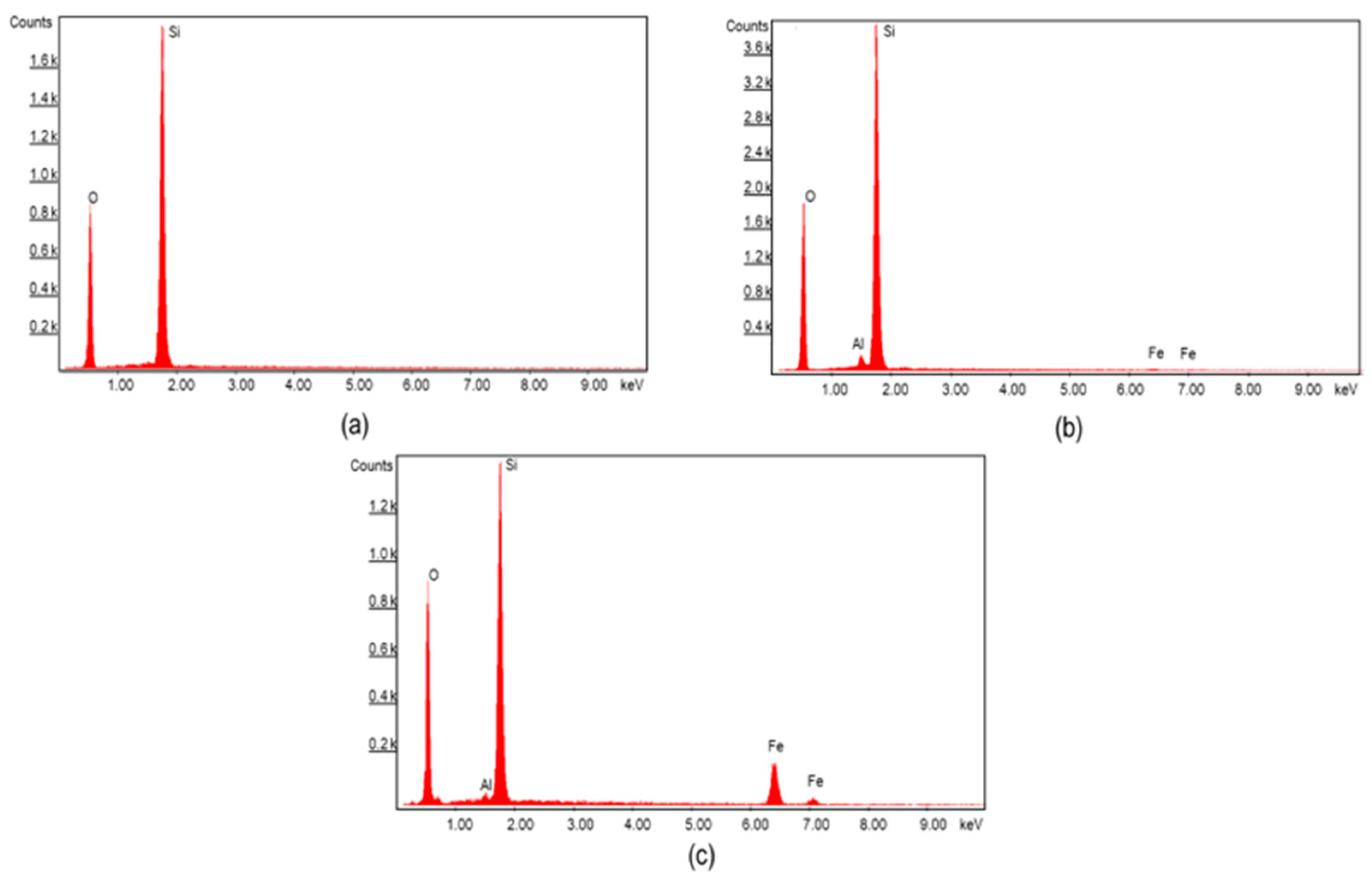
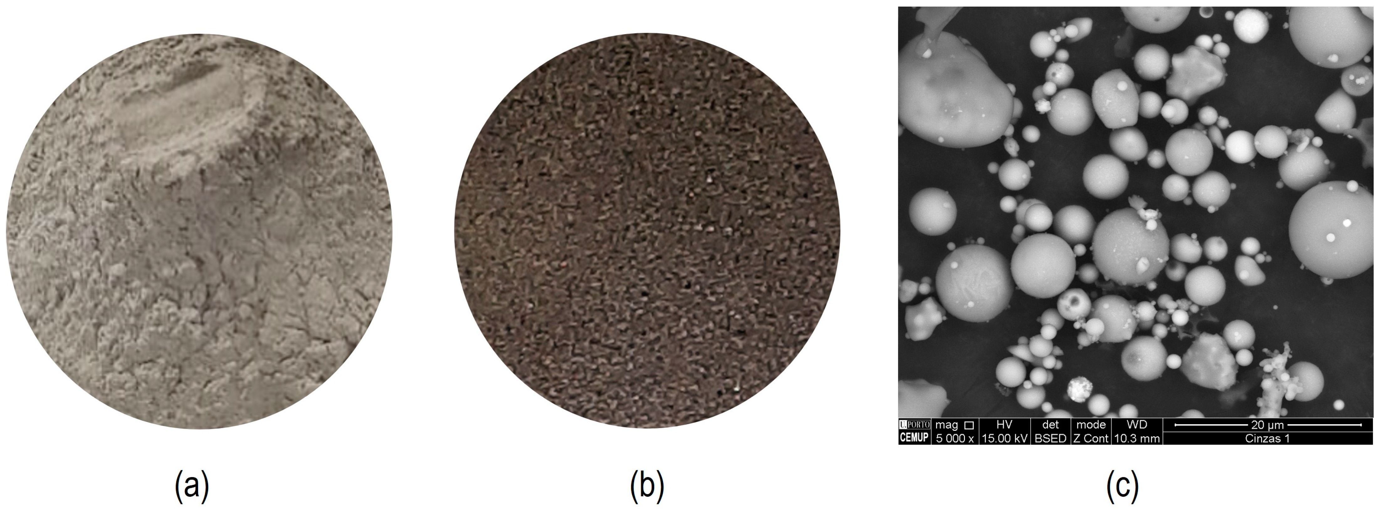
Figure 2 shows the iron tailings in their real size (a), the same image with a 100-times magnification from a regular camera (b), and the same image with 4000-times magnification obtained by SEM (c). In the imaged zoomed 4000 times, it is possible to observe the angularity of tailings particles, where the brighter particles are iron oxides. EDS analysis indicated that the iron tailings are mainly composed of iron (Fe) and silicon (Si), with many of its particles coated with aluminum (Al) and iron (Fe) particles, as can be seen in Figure 3 and Figure 4.
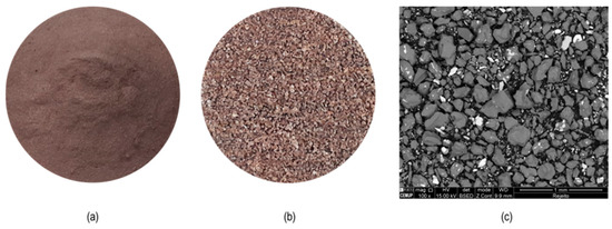
Figure 2.
Iron ore tailings: (a) real size, (b) zoom 100×, and (c) zoom 4000×.
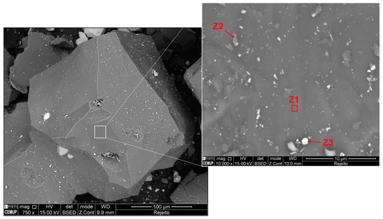
Figure 3.
Identification of regions analyzed by EDS on iron tailing.
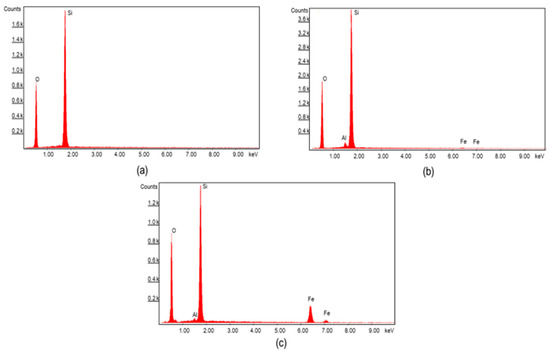
Figure 4.
EDS results on the points indicated in Figure 3: (a) Z1, (b) Z2, and (c) Z3.
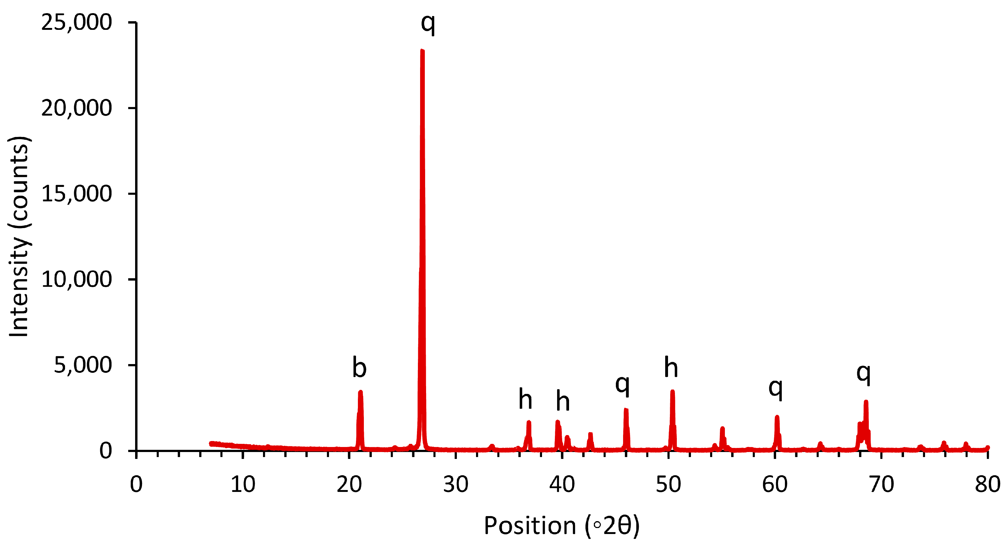
The XRD analysis identified the main minerals present in the iron tailings: proto-hematite (7.7%), low quartz (91.4%), and berlinite (0.9%), as illustrated in Figure 5.
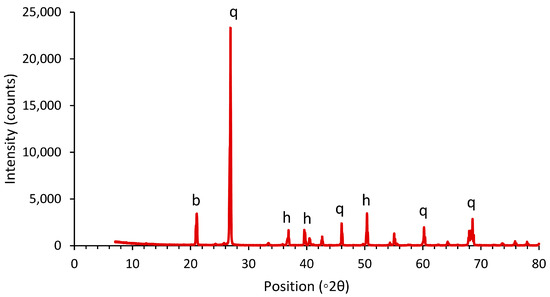
Figure 5.
XRD analysis of the iron tailings (b = berlinite; h = hematite; q = quartz).
Figure 6 shows the fly ash in the real size (a), its image with 80-times magnification from a regular camera (b), and its image with 8,000,000-times magnification obtained by SEM (c).

Figure 6.
Fly ash type F: (a) real size, (b) zoom 80×, and (c) zoom 8,000,000×.
The SEM micrograph illustrates the typical spherical shape of the fly ash particles (Figure 6c), resulting from their production method, where they come to a solid state while in suspension. However, Figure 6c also shows some angular particles, which, based on EDS analyses, could be coal. In fact, the EDS analysis indicated not only the possible presence of coal but also calcium carbonates among fly ash components.
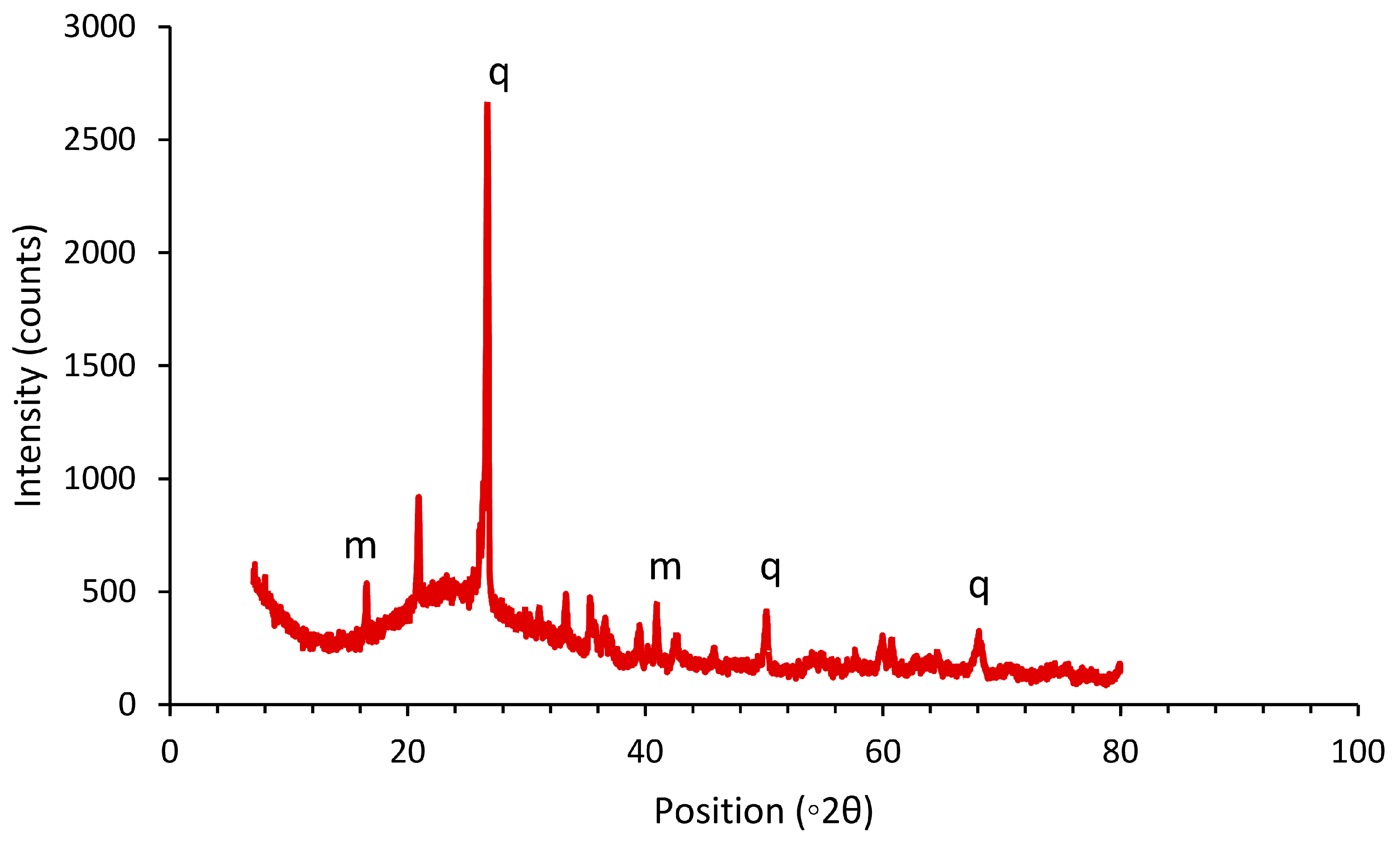
The main minerals present in the fly ash obtained in the XRD analysis were quartz (54.7%) and mullite (45.3%), as can be seen in Figure 7.
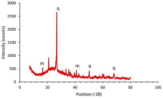
Figure 7.
XRD analysis of the fly ash (m = mullite; q = quartz).
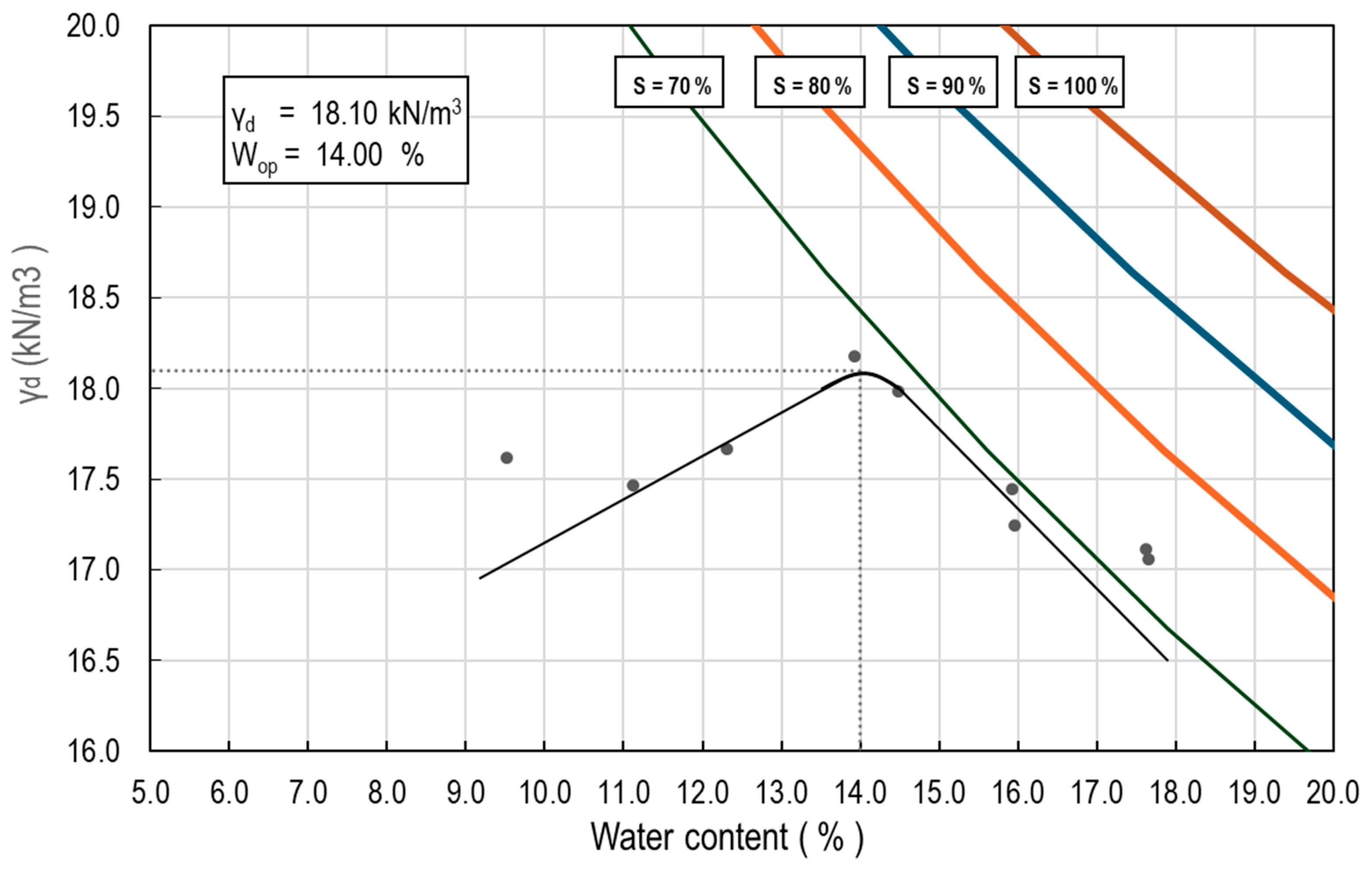
To evaluate the compaction properties of the iron tailings, a Standard Proctor test [25] was performed, whose compaction curve is presented in Figure 8. The obtained optimum water content was 14%, and the maximum dry unit weight (γd) was 18.1 kN/m3. In the same graph, the curves for different saturation degrees are included, indicating that the wet branch of the compaction curve has approximately a degree of saturation of 70%.
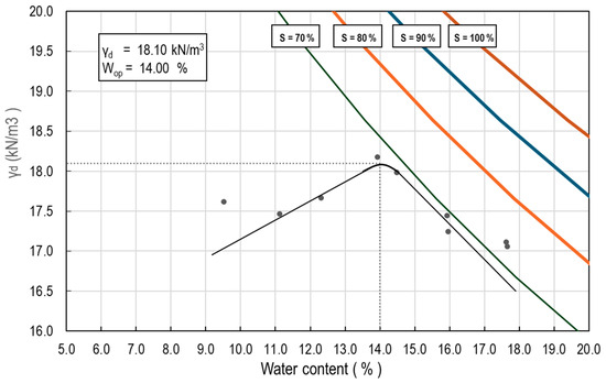
Figure 8.
Standard Proctor test in the iron tailings.
2.2. Description of the Statistical Model
A statistical methodology based on the response surface method (RSM) was used to obtain a suitable mathematical model for predicting the maximum peak strength of the material resulting from different mixtures. The Design of Experiments (DOE) underneath the RSM [20] minimizes the number of required experiments while providing an efficient tool for data analysis and interpretation, therefore allowing efficiency and economy in the experimental process and scientific objectivity in the resulting conclusions.
Three input variables were considered: ash content (tFA), liquid content (tL), and activator concentration (cSH). The quantity tFA is given by the mass ratio of fly ash with the iron tailings; tL is the liquids-to-solids ratio in the mixture given by the mass of sodium hydroxide and water divided by the mass of soil and fly ash, and cSH is the molal concentration of sodium hydroxide solution. The range of variation for each variable in the DOE was defined based on preliminary tests. These intervals are presented in Table 2.
Table 2.
Range of values used for each variable in the DOE.
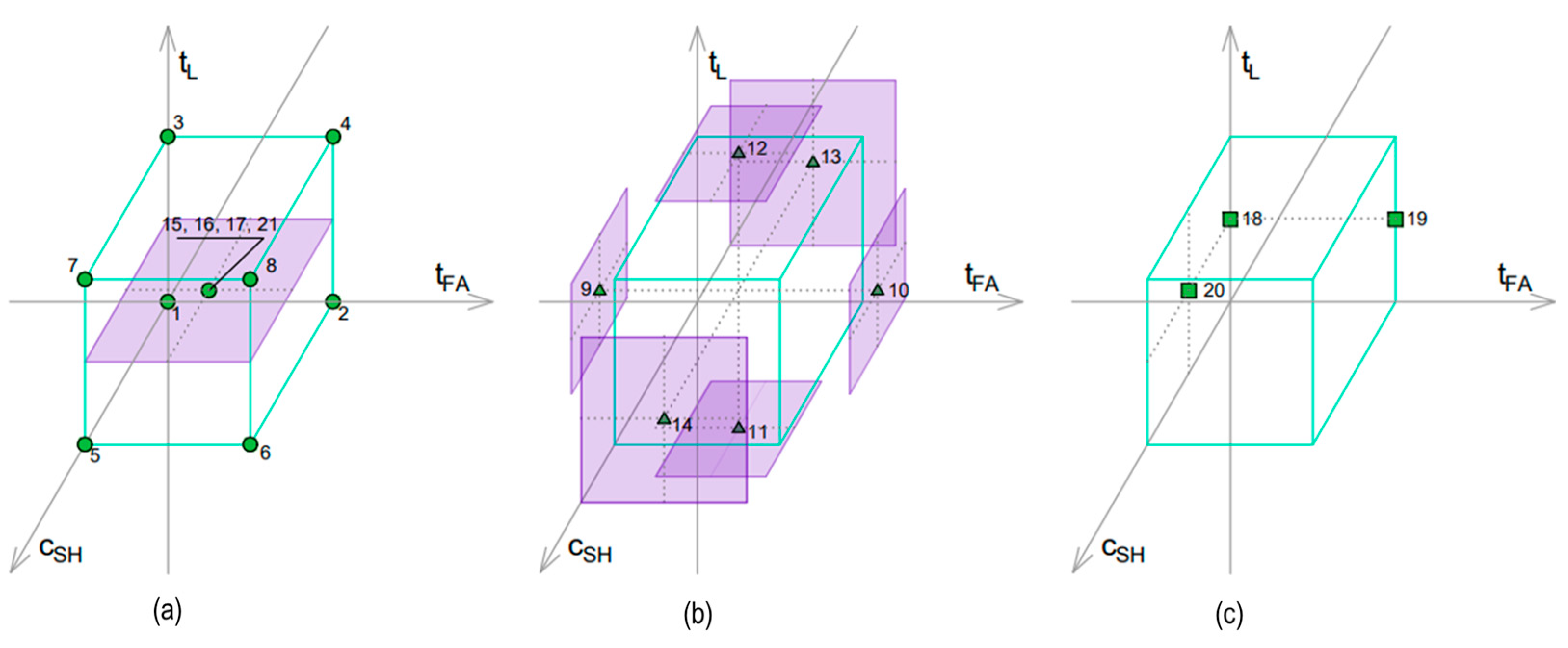
Based on these input variables and their range, a set of mixtures to be tested is proposed which constitutes the plan of experiments undertaken and reported in the present paper. The set of mixtures, in a total of 21 runs, is presented in Table 3 and depicted in Figure 9. The designed plan is a factorial plan composed of 8 factorial runs plus 4 central runs (Figure 9a) augmented with 6 axial runs (Figure 9b) and 3 middle plane runs (Figure 9c); see [20].
Table 3.
Mixtures from each phase of the statistical model.

Figure 9.
Points of the statistical plan in the space tL, tFA, and cSH in each phase: (a) factorial and central runs, (b) axial runs, and (c) middle plane runs.
The output variable considered in this work was the maximum peak strength (qu) obtained in the unconfined compressive strength (UCS) test.
2.3. Specimen Preparation and Testing Procedure
Mine tailings that come from the ore-processing plant are in a slurry, which passes through a filter to reduce the water content to approximately 17 to 23%. For this reason, this work intended to simulate the wet tailings as they come from the filter plant.
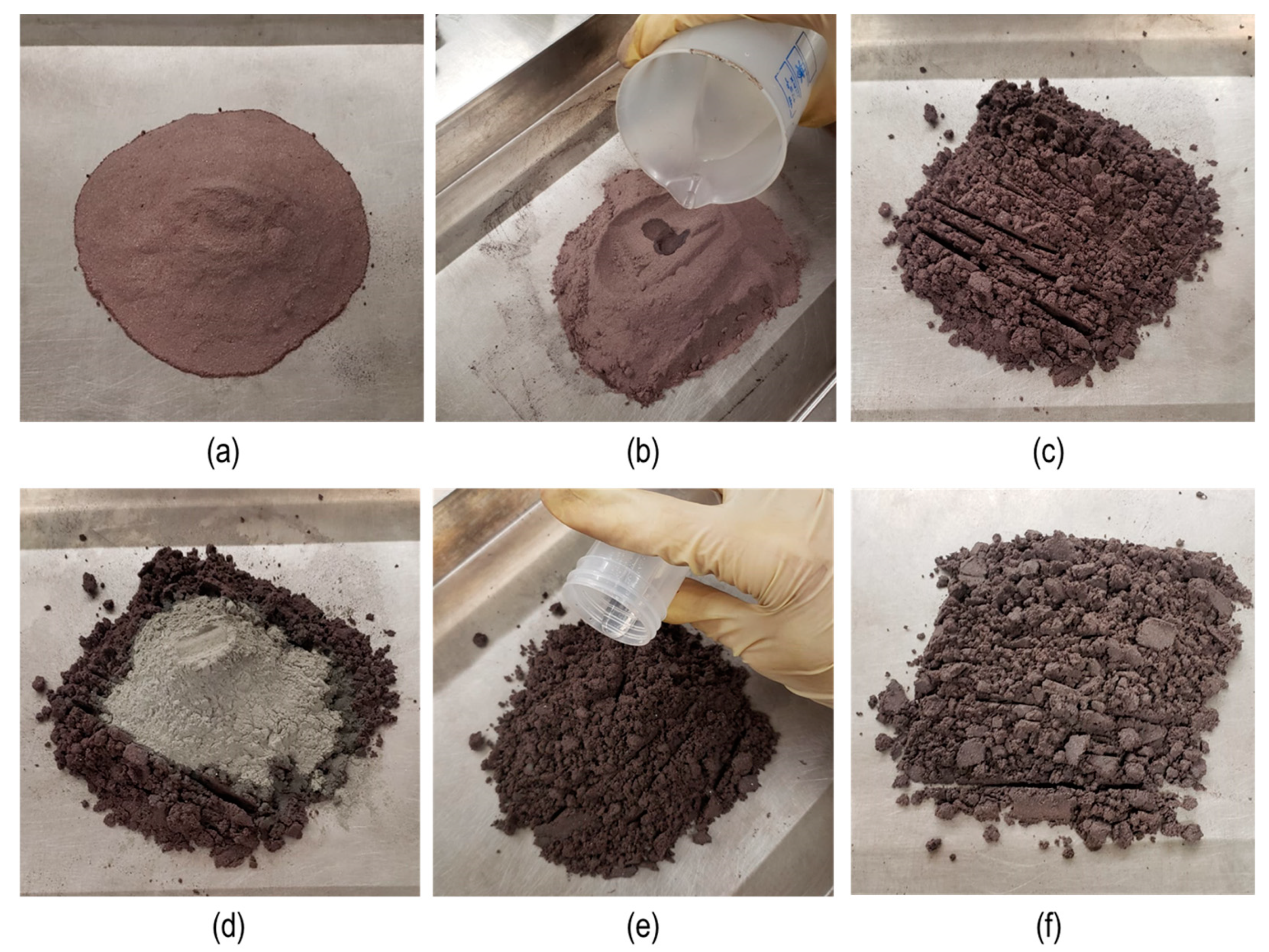
Therefore, 15 mL of water was added to the oven-dried tailings for each mixture combination. With the water incorporated into the tailings, fly ash was added and mixed until full homogenization. This process is not only more realistic but has also the advantage of releasing less dust during mixing. Then, sodium hydroxide solution (activator) was added with further homogenization before transferring the final mixture to a sealed plastic container to minimize liquid loss. This mixture preparation methodology is shown in Figure 10.

Figure 10.
Methodology of mixture preparation: (a) dry tailings, (b) water added to simulate the filtered tailings conditions, (c) tailings and water homogenized, (d) fly ash added, (e) SH solution added, and (f) final mixture.
Due to the initial added water, the concentration of sodium hydroxide in the solution was diluted, with the actual concentration (cA) being calculated using Equation (1):
where mSHs is the mass of solid sodium hydroxide in the activator, mw is the initial mass of water added, and mwSH is the mass of water present in the activator.
The specimens were prepared in molds of 36 mm in diameter and 66 mm in height by static compaction in three layers targeting a dry unit weight, γd, equal to 17.2 kN/m3, which corresponds to 95% compaction degree compared to the optimum unit weight presented in Figure 8. As noted by [26,27], dry stackings are usually constructed with different compaction levels in order to optimize the execution and follow the production rate, so in most cases, a 100% Proctor density is not achieved.
Demolding was carried out on the same day, using an extractor, and the specimens were subsequently stored in an insulated box for 7 days, before being tested in unconfined compression.
To evaluate if this preparation procedure was providing repeatable specimens, the porosity (η) of the specimens on the molding day was calculated using Equation (2):
where γdm is the dry unit weight of the mixture, given by Equation (3); wS, wFA, and wSHs are the dry masses of soil, fly ash, and solid sodium hydroxide in the mixture, respectively; wT is the total mass of the specimen on the molding day; γsS, γsFA, and γsSHs are the particles unit weight of soil, fly ash, and solid sodium hydroxide; V is the volume of the specimen; and tL is the liquid content.
The unconfined compression strength test (UCS) performed was based on ASTM D2166-06 [28] using a 20 kN load cell with a ball joint to ensure vertical load application, and a linear variable differential transformer (LVDT) for vertical strain measurement.
From the UCS test, the stress–strain curve of the specimens was obtained, as well as the values for the maximum peak strength (qu), given by Equation (4):
where Fmáx is the peak load registered, and Acorr is the corrected area due to the radial deformation of the specimen during the compression. This area is calculated by using Equation (5), based on [29]:
where D is the specimen diameter, and εa is the axial deformation in the moment of the maximum strength, given by the ratio of the height variation by the initial high of the specimen (ΔH/H0).
3. Results and Discussion
3.1. Evaluation of Specimen Preparation Procedure
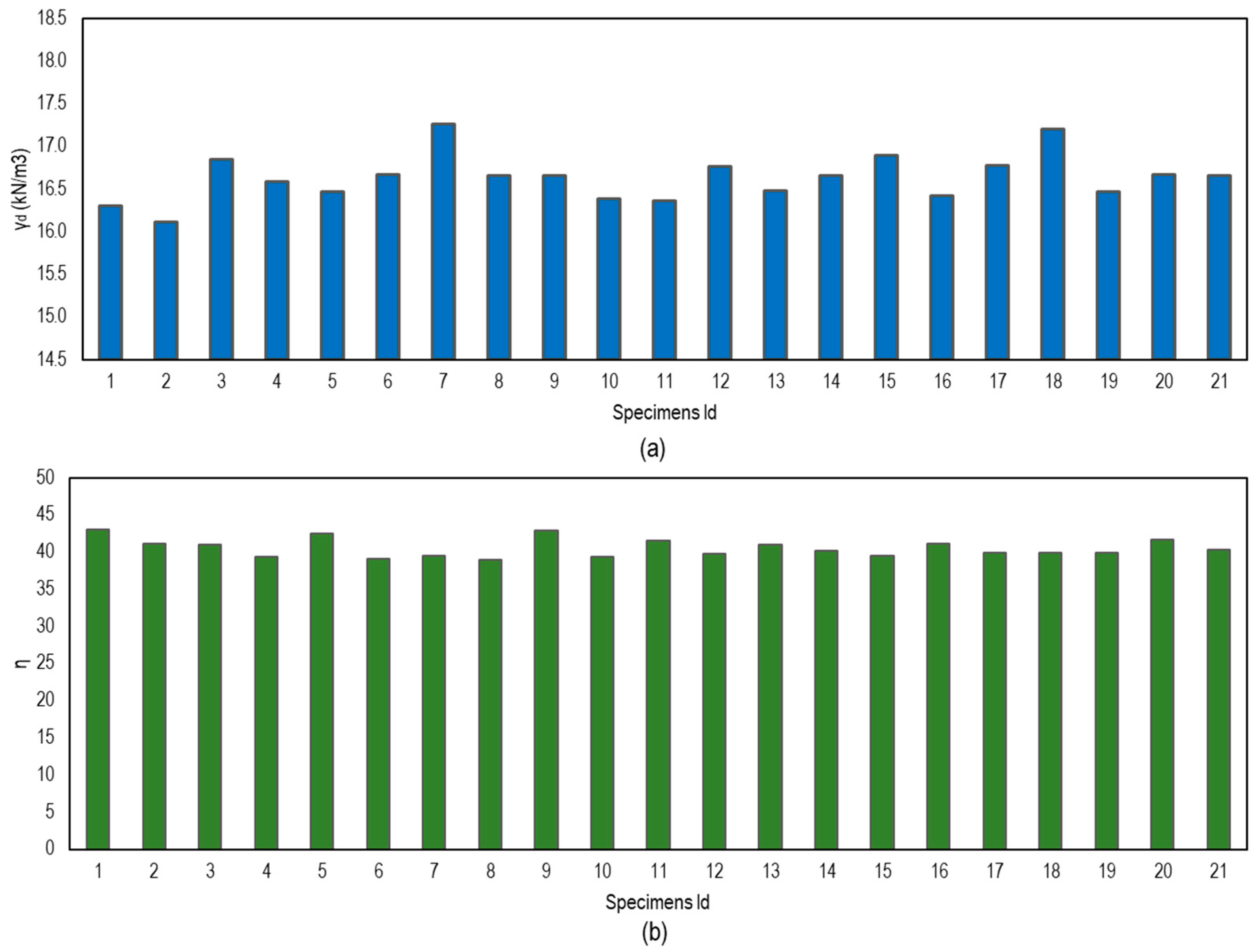
Figure 11 presents both the dry unit weight (γd) and porosity (η) on the day of specimen preparation. The results show that the dry unit weight is slightly lower than the target value (17.2 kN/m3), which may be due to water evaporation from the mixture during molding. However, when analyzing the porosity values for each specimen, it can be observed that the variation was quite low (approximately 4%). These results confirm the suitability of the specimen preparation procedure to obtain specimens with similar void ratios, so that the measured strength will depend only on mixture composition.

Figure 11.
Molding parameters for the mixtures on the day of specimen preparation: (a) dry bulk density (γd) and (b) porosity (η).
Table 4 provides a statistical summary of the results consisting of the maximum, minimum, amplitude, and average values of the measured parameters in this set of mixtures. The analyzed parameters include the initial moisture content of the tailings (w0), the total moisture content (w), γd, and η. The parameter w0 was calculated considering only the initially added water divided by the mass of tailings in the mixture. The parameter w was calculated considering the total water involved in the process, including that of the sodium hydroxide solution, divided by the tailings’ dry weight.
Table 4.
Summary of parameters on molding day of the specimens.
During the 7 days of curing time, the specimens were stored in an insulated box that minimized the influence of external factors. Nevertheless, they showed variations in mass (Δm), as seen in Figure 12. It was noticed that this variation was positive, meaning that there was weight loss for all specimens except for specimen 12, whose mass increased after 7 days. These mass variations may be due to the chemical reactions involved in the alkaline activation explaining the differences in each mixture.
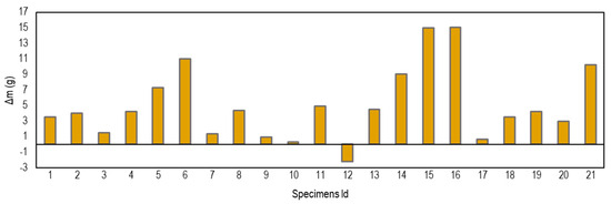
Figure 12.
Mass variation in the specimens along 7 days inside an insulated box.
3.2. Unconfined Compressive Strength
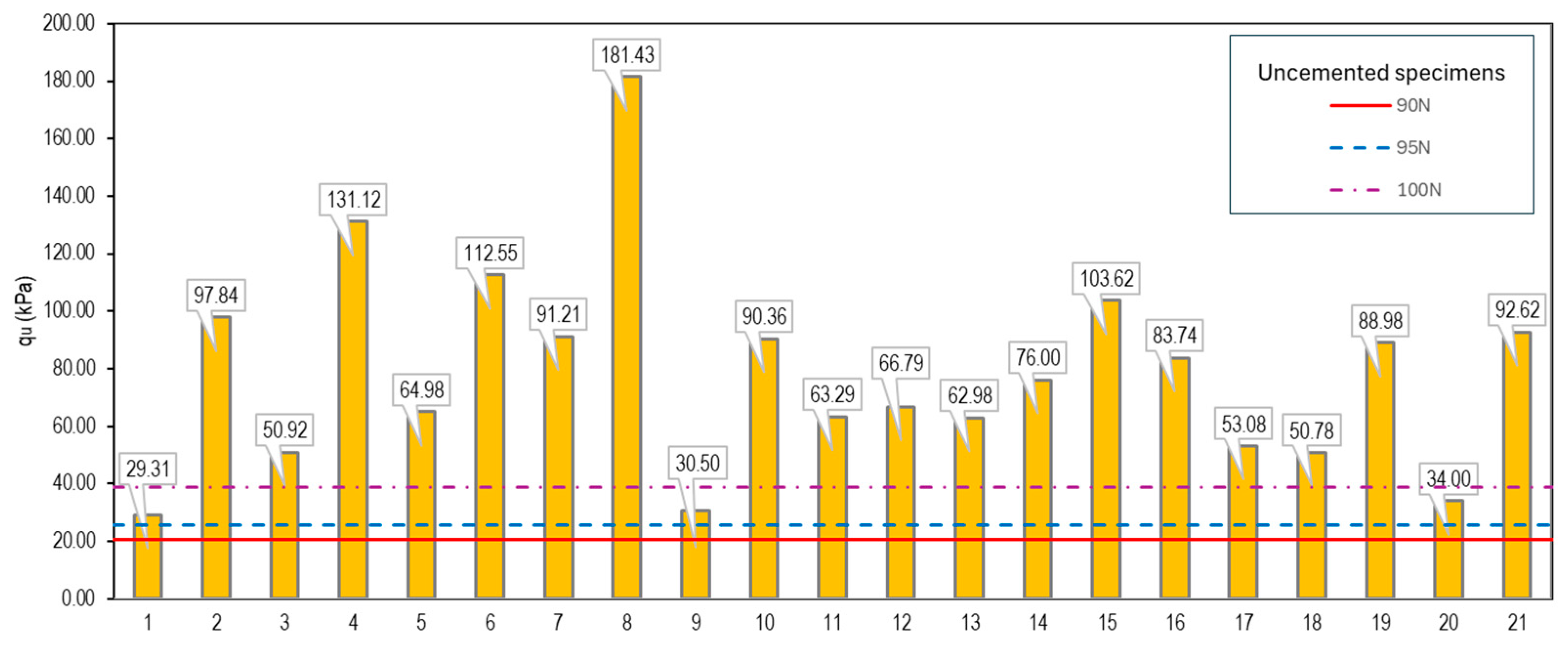
The maximum peak strength (qu), measured in the unconfined compression strength test, of the treated mixtures defined in Table 3 is shown in Figure 13, along with the qu results obtained for the untreated tailings. The full dataset is also available as a supplementary data file. For comparative purposes, three different compaction degrees were used in the untreated tailings, whose results are also presented in Figure 13. The specimen that exhibited the highest strength corresponds to mixture 8, which attained the extreme values of each variable. Specimens with lower strength were specimens 1—with the lowest limit values of variables—and 9, which has the lowest tFA value. All specimens showed qu values higher than those of the untreated tailings compacted at 90% and 95% of the Standard Proctor, and only two mixtures (numbered 1 and 9) presented values below the strength obtained in the untreated tailings compacted at 100% of the Standard Proctor. Therefore, it becomes clear from these results that there is a significant improvement in strength due to the stabilization with alkali-activated fly ash in comparison to the untreated tailings. In mixture 8, this improvement corresponds to approximately eight times the untreated strength.
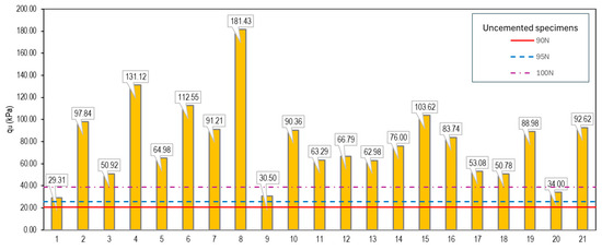
Figure 13.
Unconfined compression strength of all mixtures tested after 7 days of curing, along with the strength of the untreated tailings compacted at 90%, 95%, and 100% degree of compaction (Standard Proctor).
Since the results presented in Figure 13 showed a trend of increasing strength with greater values of the mixture parameters, the possibility to expand the experimental plan by increasing the upper range of the input values was considered. However, this option was not reasonable for the following reasons: (1) Increasing the fly ash content (tFA) would increase the precursor amount beyond reasonable limits, and, therefore, it would increase the volume of the material in the dry-stack pile. (2) Increasing the liquid content (tL) makes it unfeasible to control the liquid content of the laboratory specimen since the liquid comes out from the specimen at the base and top of the mold during compaction, indicating that the mixture is close to saturation. (3) Increasing the concentration of the SH solution could lead to operational issues in situ, requiring additional care to perform the mixture, and a higher carbon footprint. On the other hand, it should be noted that, for the purpose of slope stabilization, very high unconfined compression strengths may not be required [30].
3.3. Statistical Modeling
3.3.1. Fitted Models
Although the main output target of the statistical analysis was the maximum peak strength of the unconfined compression strength test (qu) and its dependence on tFA, tL, and cSH, other parameters were analyzed to find any possible relationships. Among the analyzed parameters are the actual concentration of the mixture (cA, given by Equation (1)), the variation mass of the specimens on the molding and testing days (Δm), and the variation in environmental temperature on the molding and testing days (Δt). Based on an initial statistical analysis (hypothesis testing), the following conclusions were drawn:
- The actual concentration (cA) of the mixture is highly dependent on the variable tL (r = 0.841, p < 0.1%); therefore, its inclusion as an input parameter to the statistical model together with tL is not possible;
- There is no significant correlation between qu values and the mass variation (Δm) during curing. The p-value associated with the hypothesis of no correlation between these parameters is equal to 22.1%; therefore, there is no evidence of correlation between qu and Δm;
- The factor that most contributes to the maximum peak strength response is tFA, followed at some distance by the cSH and the tL. The tL is the least important factor of the three in explaining the response, although it is still significant (p-value = 4.9%).
A significance level of 5% was considered in all statistical analyses. A subsequent statistical regression analysis led to two statistical models which can be used to predict the strength response. They are denoted here as Model 1 and Model 2. A logarithm transformation to the response data is needed to fit a regression model properly.
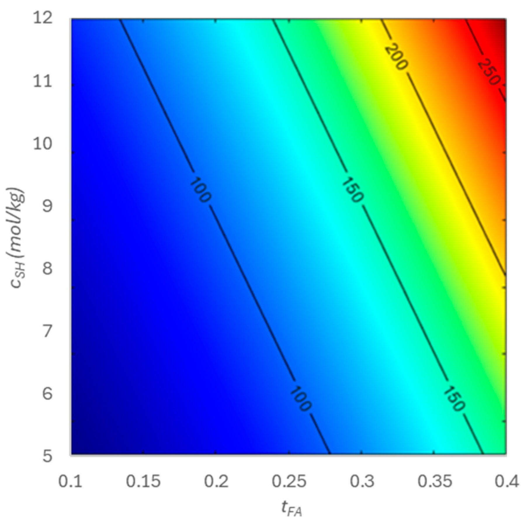
In Model 1, the three input variables intervened (tFA, tL, and cSH), as expressed in Equation (6). The obtained model is loglinear, as all interactions between variables and non-linearities were not significant (p-value > 10% for all interactions analyzed). Figure 14 shows the growth trend of qu according to Model 1, based on the variables fly ash content (tFA) and SH concentration (cSH), which are the most significant variables driving qu. In this case, the variable tL was fixed at 0.17. Higher strengths are in the upper right corner: there is an increase in qu with both input variables.

Figure 14.
The maximum peak strength as a function of tFA and cSH.
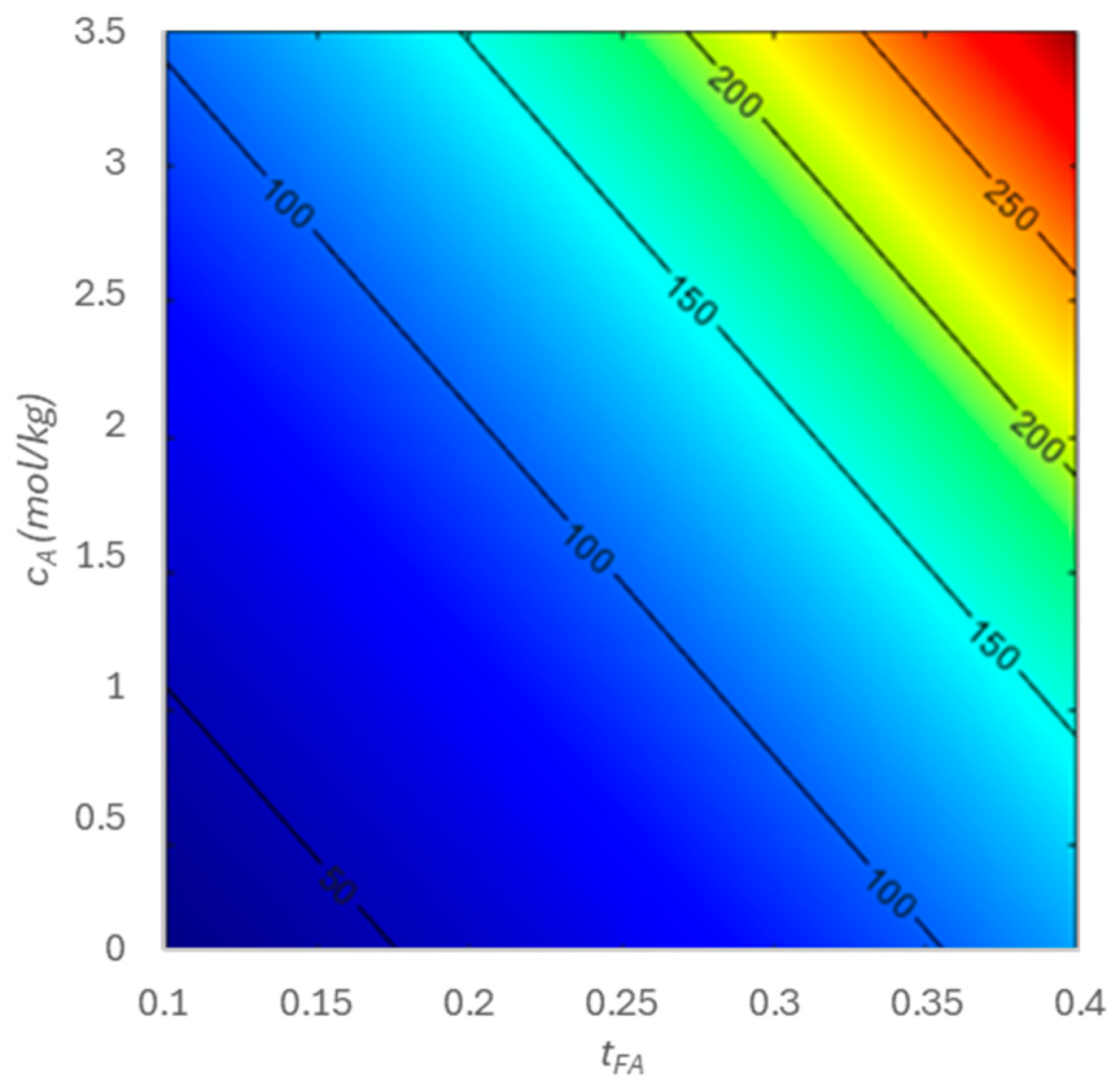
Model 2 has the advantage of using only two variables, as expressed in Equation (7). Figure 15 shows the growth trend of qu based on the variables fly ash content (tFA) and actual sodium hydroxide concentration (cA) calculated by Equation (1).
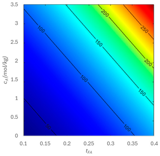
Figure 15.
The maximum peak strength as a function of tFA and cA.
3.3.2. Performance Measures
The assessment of the model fitting was performed based on five measures: R2, adjusted R2, Akaike Information Criteria (AIC), and Bayesian Information Criteria (BIC). These measures are commonly adopted as performance measures in statistical modelling (see, e.g., [31]). Their obtained values can be read in Table 5.
Table 5.
Performances measures for Models 1 and 2.
The R2 is the most common measure to evaluate the explanatory ability of a regression model. It represents the proportion of the variance of a dependent variable that is explained by one more independent variable in a regression model [32]. Therefore, the higher the value of R2, the higher the expected explanatory power of the input variables should be. In both models, a high R2 was not achieved, with the first being equal to 0.735 and the second to 0.743. The pair tFA and cA explains the material response slightly better than the pair tFA and cSH, and this may be because cA includes the whole liquid phase inside the specimen responsible for the alkali activation reactions.
The adjusted R2 (R2adj) is a measure of the goodness of fit (accuracy of the model) corrected for linear models. While R2 tends to optimistically estimate the fit of a linear regression, always increasing as the number of effects included in the model increases, R2adj attempts to correct this overestimation. For this reason, it is always smaller or equal to R2 [32]. The R2adj is slightly higher in Model 2 (0.715) than in Model 1 (0.688), suggesting that Model 2 provides a better fit.
The Akaike Information Criterion (AIC) provides a mathematical tool for evaluating how well a model fits the data, but mostly it can be used to compare different possible models and determine which one is the best fit for the data [33]. This measure helps in assessing whether it is useful to add another parameter to the model. For Model 1, the AIC is equal to −25.7, and the AIC is equal to −43.2 for Model 2. The ratio between AIC values is 1.68, indicating that the model with the lowest AIC value (Model 2) should be preferred.
Similarly to the previous measure, the Bayesian Information Criterion (BIC) can also be used to assess two competing models. The literature proposes different practical rules to be adopted when comparing fitted models based on BIC (see, e.g., [32]), and the model with the lowest BIC should be retained. The values presented in Table 5 suggest that Model 2 would provide the best fit.
3.3.3. Validation of the Fitted Models
To assess to what extent the proposed models can predict the strength of a given mixture, a validation phase was performed where 10 new mixtures were tested (Table 6). Some of the mixtures had input variables extrapolated outside the initial range expressed in Table 2 to explore regions with higher qu values. However, there is no interest in increasing the tFA variable, as it would make its practical use unfeasible. Thus, the extrapolation was mostly in the variables tL and cSH. To achieve higher values of the SH concentration, the initially added water was reduced.
Table 6.
Validation phases of the model and their respective qu.
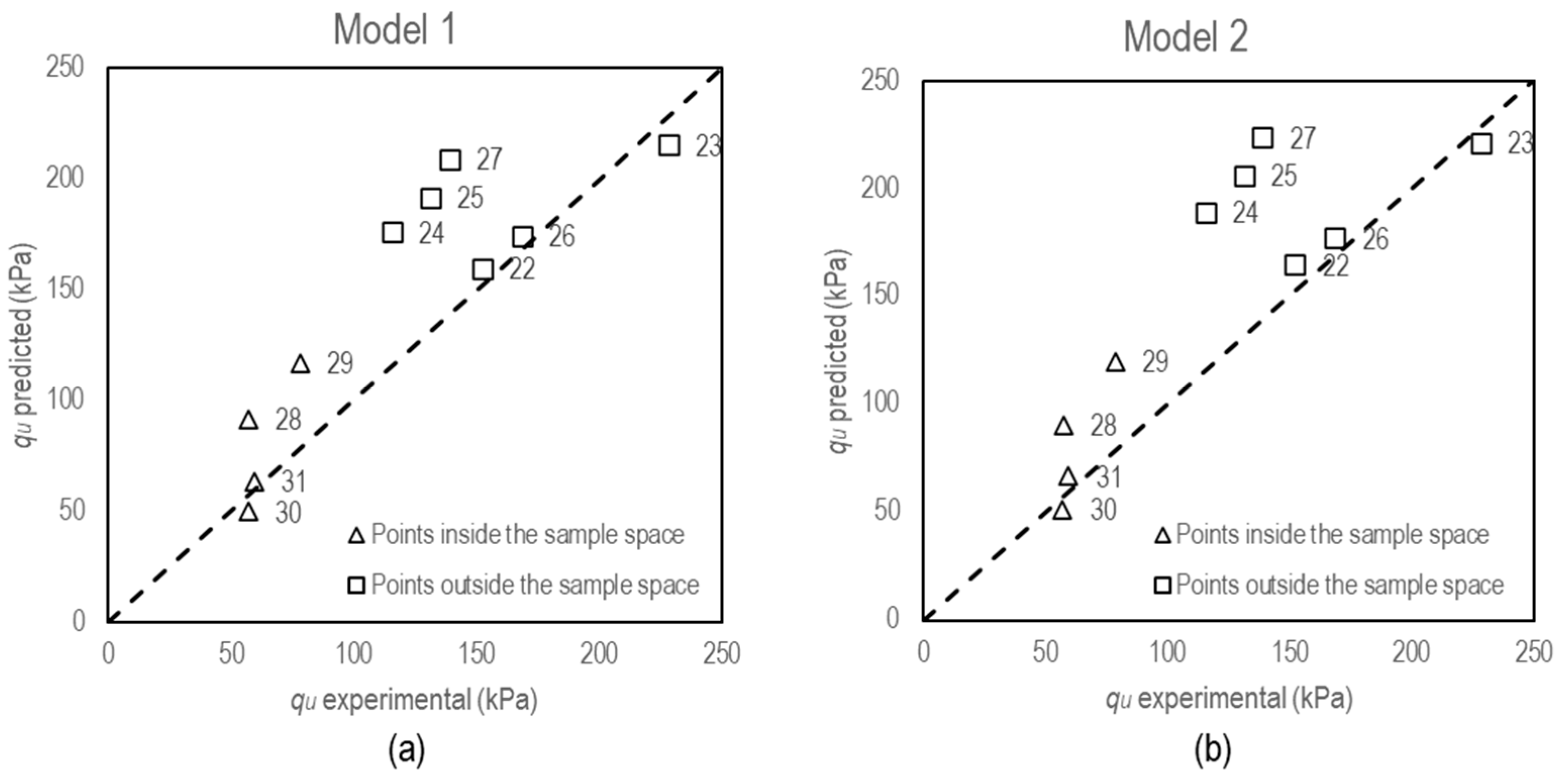
Figure 16 shows the comparison between the experimental and predicted values of qu for both models, (a) Model 1 and (b) Model 2, using the 10 validation points expressed in Table 5. In short, the closer the points are to the diagonal line of Figure 16 and placed randomly on both sides of the line, the better the model is.

Figure 16.
Experimental x predicted points according to (a) Model 1 and (b) Model 2. The numbers indicated next to the marker correspond to the ID number given in Table 5.
From the results, the following was observed:
- For both models, all experimental qu values fall inside the 95% predicted intervals, showing a good agreement with the fitted models;
- The error between the experimental and the predicted qu values is not large;
The Root Mean Square Error (RMSE) measures the average deviation between a statistical model’s predicted values and the actual values. In other words, RMSE quantifies how dispersed the model residuals are, revealing how tightly the observed data clusters are around the predicted values [32]. RMSE can be used to compare the effectiveness of models by testing their prediction capability on points that were not used in model fitting, namely validation points. The lower the value of RMSE, the closer the data points are to the regression curve, resulting in greater accuracy of the model. In our framework, considering all 10 data points of the validation phase, the RMSE is smaller for Model 1 (43.11 kPa) than for Model 2 (55.44 kPa). However, considering just the six validation runs that do not go far outside the sample space (i.e., points 22, 24, 28, 29, 30, and 31), the RMSE decreases considerably in both Model 1 (RMSE = 28.11 kPa) and Model 2 (RMSE = 30.37 kPa). This could indicate that the models can predict well near the region associated with the initially considered range (see Table 2).
Notice that, according to Figure 16, in both models, there are three points that do not fall inside the initial boundaries of the plan (marked with squares) and are farther away from the diagonal line. These points are numbered 24, 25, and 27, and their liquid content (tL) is the same and equal to 0.18. In these points, both models predict higher strengths when compared to experimental values. A possible explanation may be that, for the studied region (tL ∈ 0.14–0.17), a linear behavior was found; meanwhile, beyond that initial range, the relation may be nonlinear. If these three points were excluded from the initial set of 10 runs, the RMSE values would decrease considerably in both models (respectively, equal to 19.05 kPa for Model 1 and 6.65 kPa for Model 2). Therefore, Model 2 is proposed to predict qu inside the sample region. A further investigation is needed to refine the dependence of qu, for very high values of tFA and cSH or the cA. That was not the intention of the present experimental plan, due to limitations in the practical implementation of the mentioned mixtures.
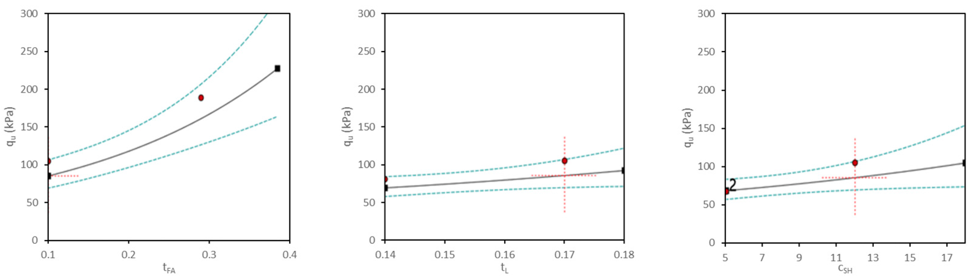
Figure 17 illustrates how fast the optimum qu can be achieved by increasing the values of tFA, tL, or cSH. Although the maximum strength is achieved when higher values of the input variables are used, Figure 17 highlights the fact that the fly ash content has a much higher influence on the obtained strength. As mentioned before, the behavior of the tL and cSH input variables is linear in log qu, being almost flat.
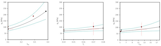
Figure 17.
Strength evolution depending on the individual variation in each input variable.
3.4. Definition of a Mixture Index
In an attempt to obtain a single index that would represent the mixture composition and that could explain the strength values well, a commonly used parameter for cemented soils [15,16] was investigated: the volumetric cement content, Civ, given by Equation (8):
where Vc is the cement volume given by Equation (9), and V is the specimen volume.
where wFA is the fly ash weight; wSHs is the solid sodium hydroxide weight; and γsFA and γsSHs are the particles unit weight of fly ash and solid sodium hydroxide, respectively.
After calculating the Civ for the mixtures indicated in Table 3 and Table 6, another statistical model, denoted Model 3, was therefore obtained by Equation (10):
The volumetric cement content is currently used together with the mixture porosity, in the so-called porosity/cement ratio, as the effectiveness of cementation also depends on the number of contact points between particles [15]. Applying this other index to the data presented in Table 3 and Table 6, following the same type of mathematical equation proposed by [34], led to the model proposed in Equation (11) (Model 4).
If another type of appropriate mathematical function is used (“S” curve), a slightly better fit is found, as given by Equation (12) (Model 5).
Table 7 summarizes the values of the coefficient of determination (R2) and R2 adjusted associated with Models 3, 4, and 5, from which the following comments follow:
Table 7.
Coefficient of determination of Models 3, 4, and 5.
- Models 3 to 5 provide similar coefficients of determination, all of the three slightly higher than those of the previous models (Models 1 and 2);
- Even in an experimental plan where all the mixtures have approximately the same porosity (see Figure 11), the porosity/cement ratio (Model 4) seems to perform slightly better than Civ (Model 3);
- Model 5 has slightly higher values of R2 and R2adj, and the estimates of the constants in the model are not very large values, as is the case on the other models (e.g., 1013.795 in Model 4), which is in favor of Model 5 for practical use.
In obtaining all the three expressions above (Models 3, 4, and 5), it was checked that assumptions of the regression modelling regarding residuals, outliers, and leverage points hold.
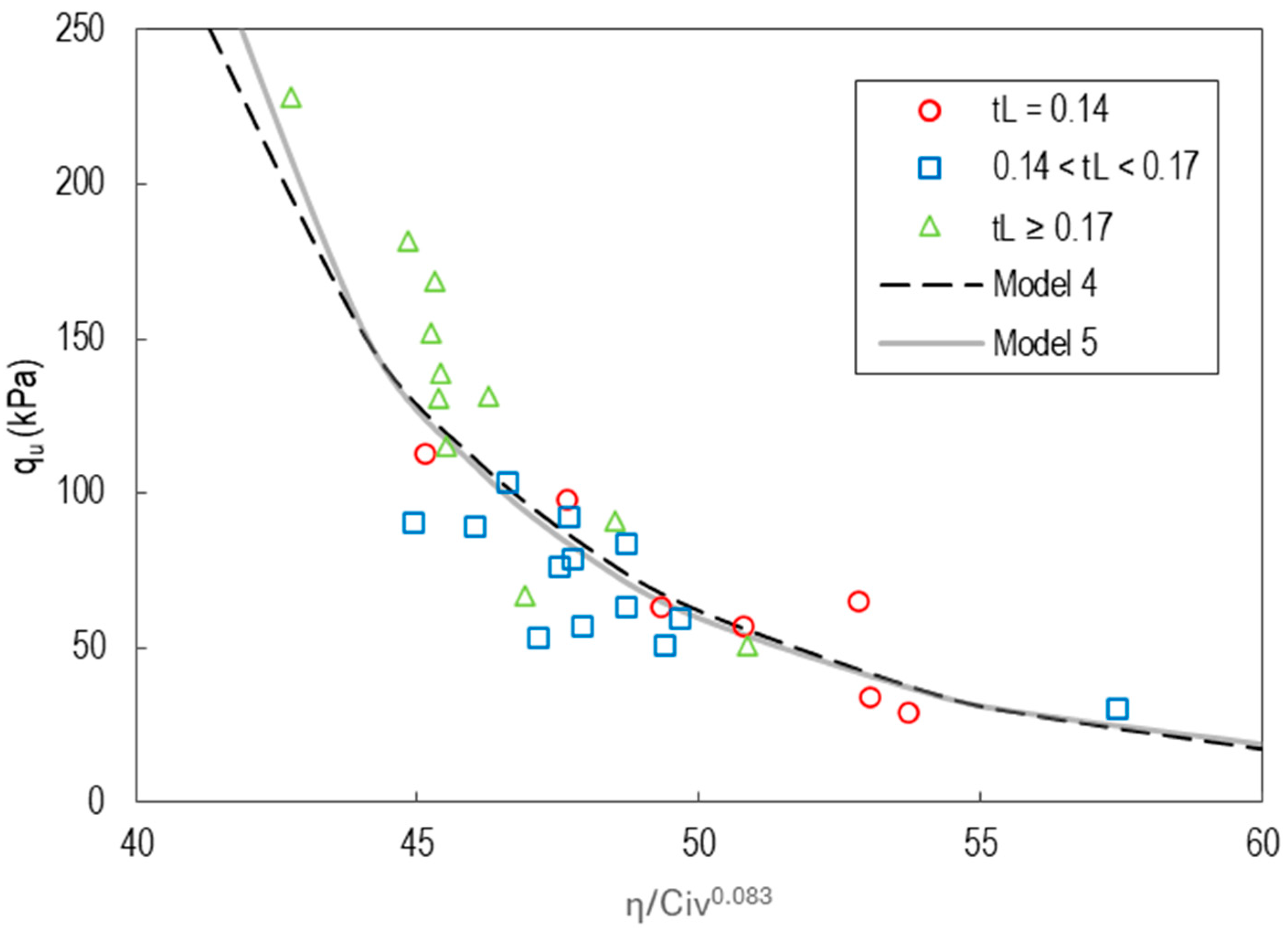
Considering that, in this experimental plan, the water content and liquid content of the mixtures were not constant at the optimum points, as in previous studies [18,34], several attempts were made to include this effect on the mixture index. In a preliminary approach, the experimental points were plotted together with Models 4 and 5 (see Figure 18), using a different marker for mixtures associated with each liquid content to evaluate if the mixtures with certain liquid contents would be farther away from the model curve. From Figure 18, it seems that the scatter is similar for all liquid contents.

Figure 18.
Models 4 and 5 and experimental points marked according to the value of tL.
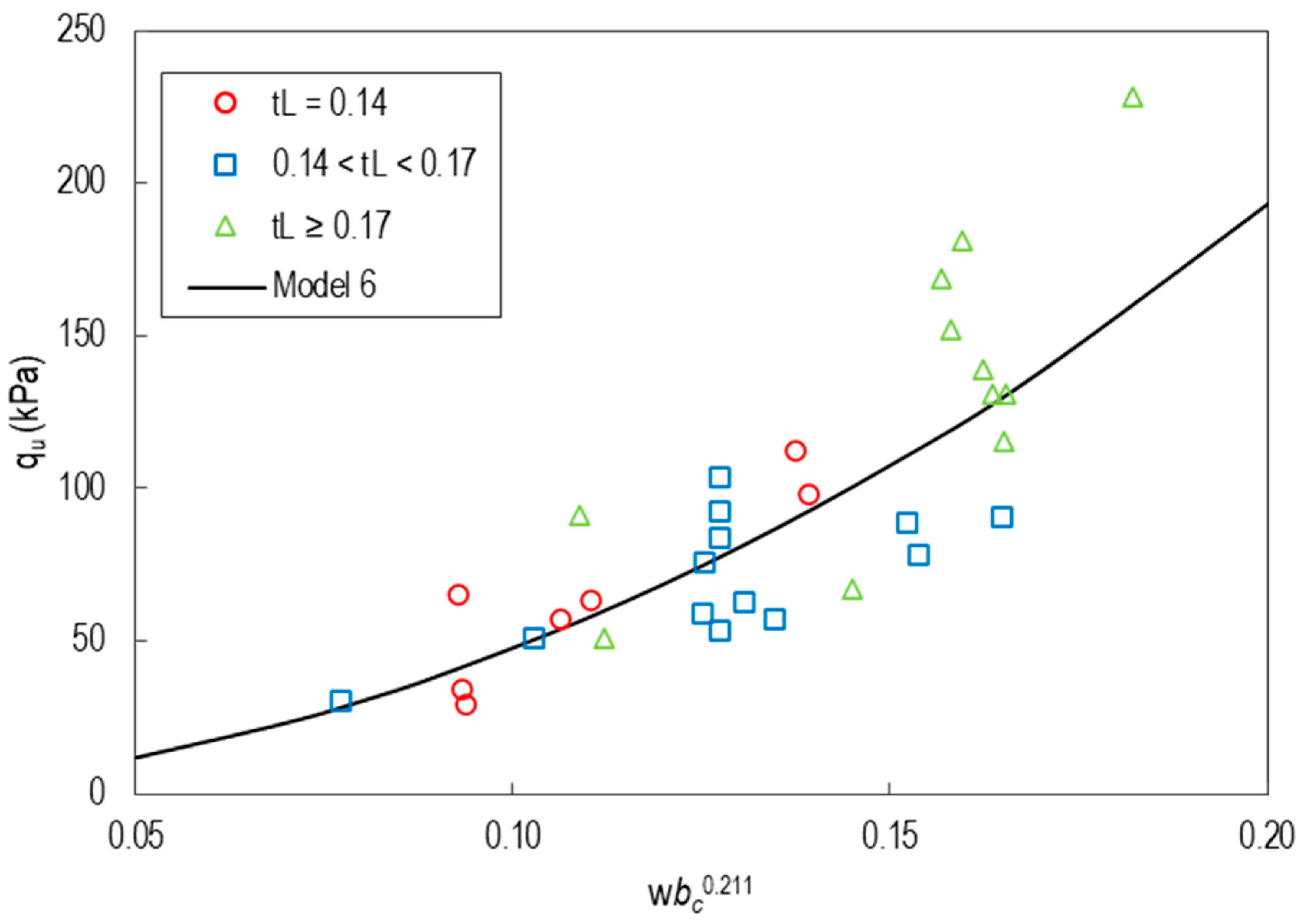
Subsequently, other indexes were evaluated. One of the indexes analyzed (w/bcn) is based on the two mass ratios defined in Equations (13) and (14), the water content (w) and the binder content (bc), adjusted by an exponent, n.
where ww is the water weight, ws is the soil weight, wFA is the fly ash weight, and wSHs is the sodium hydroxide solid weight. For this index, Model 6 was fitted as expressed in Equation (15).
Its curve is shown in Figure 19.
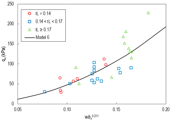
Figure 19.
Curve given by Model 6 and the actual qu for all points marked according to the values of tL.
Model 6 provides the worst fit when compared to previous models. This is expressed by low values of R2 and R2adj. (see Table 8). From these results, it can be concluded that, even when the liquid content/water content varies, the index proposed [15] remains valid and capable of providing a better explanation for strength prediction than other input variables that are based on water content or liquid content. This may be explained by the small liquid content range of this experimental data set which was defined by the experimental feasibility of the mixtures in terms of their workability and saturation level (much drier or wetter mixtures would be impossible to prepare and test).
Table 8.
Coefficients of determination for Model 6.
4. Conclusions
In this paper, a rational design methodology for iron tailings stabilized with an alkali-activated binder was pursued. The aim was to define a strength prediction model that could indicate the best tailing–binder mixture for a required strength considering both the mixture components (tailings, fly ash, and sodium hydroxide) and the tailings’ in situ water content. For that purpose, an experimental plan set by a response surface method was conducted which served for a further statistical analysis, leading to the following conclusions:
- The most influencing factor on the unconfined compression strength was the fly ash content, although the sodium hydroxide concentration and the mixture liquid content were also significant;
- Two statistical models were initially proposed based on those three factors. Although they provide a similar performance, the second model provides a slightly better fit, having the additional advantage of requiring just two variables;
- Higher strengths were obtained when the input variables were on the upper values of their range, but when tests were performed outside this range, the strength decreased, suggesting a nonlinear relation outside the initial interval;
- Towards the definition of a mixture index that could represent the mixture components, other statistical models depending on different indexes were proposed. The best-performing model was based on the porosity/cement ratio proposed by [34], even when the mixture’s liquid content varies.
These conclusions are very important since they highlight the relevance of the porosity/cement ratio, even when other parameters besides porosity or cement content vary. However, further tests are required to evaluate whether these same trends are observed in other AAB–tailing mixtures made by other types of mine tailings (from gold, bauxite, copper, etc.) or other AAB precursors and activators.
Supplementary Materials
The following supporting information can be downloaded at: https://www.mdpi.com/article/10.3390/app14188116/s1.
Author Contributions
Conceptualization, S.R.; Methodology, P.M.-O.; Validation, P.M.-O.; Formal analysis, I.C.; Investigation, I.C.; Writing—original draft, I.C.; Writing—review & editing, S.R. and P.M.-O.; Supervision, S.R.; Funding acquisition, S.R. All authors have read and agreed to the published version of the manuscript.
Funding
This work was financially supported by Base Funding—UIDB/04708/2020 of the CONSTRUCT—Instituto de I&D em Estruturas e Construções (https://doi.org/10.54499/UIDP/04708/2020), by the project INPROVE-2022.02638.PTDC (http://doi.org/10.54499/2022.02638.PTDC), by scholarship 2022.13858.BD to the first author, and by CEECIND/04583/2017 grant to the second author (https://doi.org/10.54499/CEECIND/04583/2017/CP1399/CT0003), all funded by national funds through the FCT/MCTES (PIDDAC). The third author was partially supported by CMUP, a member of LASI, which is financed by national funds through FCT—Fundação para a Ciência e a Tecnologia—I.P., under projects with references UIDB/00144/2020 and UIDP/00144/2020.
Institutional Review Board Statement
Not applicable.
Informed Consent Statement
Not applicable.
Data Availability Statement
The original contributions presented in the study are included in the article, further inquiries can be directed to the corresponding author.
Conflicts of Interest
The authors declare no conflict of interest.
Glossary
| Acorr | corrected area due to the radial deformation of the specimen during unconfined compression |
| bc | binder content |
| cA | actual concentration |
| Civ | volumetric cement content |
| cSH | sodium hydroxide concentration |
| D | specimen diameter |
| Fmáx | peak load registered in the unconfined compression test |
| H0 | initial height of the specimen |
| mSHs | mass of solid sodium hydroxide in the activator |
| n | normal exponent |
| qu | maximum peak strength |
| tFA | fly ash content |
| tL | liquid content |
| V | volume of the specimen |
| Vc | cement volume |
| w | water content |
| wwSH | mass of water present in the activator |
| wFA | fly ash dry mass |
| ws | soil (tailings) dry mass |
| wSHs | solid sodium hydroxide mass |
| wT | total mass of the specimen on the molding day |
| ww | total mass of water in the specimen |
| ww0 | mass of initial added water |
| γ | unit weight of the mixture |
| γdm | dry unit weight of the mixture |
| γsFA | particles unit weight of fly ash |
| γsS | particles unit weight of the soil (tailings) |
| γsSHs | particles unit weight of solid sodium hydroxide |
| Δ H | height variation |
| εa | axial deformation at the maximum strength |
| η | porosity |
References
- Solé, A.G. Hydraulic Fills with Special Focus on Liquefaction. In Proceedings of the XVII ECSMGE-2019: Geotechnical Engineering Foundation of the Future, Reykjavik, Iceland, 1–6 September 2019; pp. 1–31. Available online: https://upcommons.upc.edu/handle/2117/179180 (accessed on 1 April 2022).
- Consoli, N.C.; Vogt, J.C.; Silva, J.P.S.; Chaves, H.M.; Filho, H.C.S.; Moreira, E.B.; Lotero, A. Behaviour of Compacted Filtered Iron Ore Tailings–Portland Cement Blends: New Brazilian Trend for Tailings Disposal by Stacking. Appl. Sci. 2022, 12, 836. [Google Scholar] [CrossRef]
- Rocha, J.; Filho, R.T.; Cayo-Chileno, N. Sustainable alternatives to CO2 reduction in the cement industry: A short review. Mater. Today Proc. 2022, 57, 436–439. [Google Scholar] [CrossRef]
- Rios, S.; Cristelo, N.; da Fonseca, A.V.; Ferreira, C. Structural Performance of Alkali-Activated Soil Ash versus Soil Cement. J. Mater. Civ. Eng. 2016, 28, 04015125. [Google Scholar] [CrossRef]
- Rios, S.; Ramos, C.; da Fonseca, A.V.; Cruz, N.; Rodrigues, C. Mechanical and durability properties of a soil stabilised with an alkali-activated cement. Eur. J. Environ. Civ. Eng. 2019, 23, 245–267. [Google Scholar] [CrossRef]
- Cruz, N.; Rios, S.; Fortunato, E.; Rodrigues, C.; Cruz, J.; Mateus, C.; Ramos, C. Characterization of Soil Treated with Alkali-Activated Cement in Large-Scale Specimens. Geotech. Test. J. 2017, 40, 20160211. [Google Scholar] [CrossRef]
- Ślosarczyk, A.; Fořt, J.; Klapiszewska, I.; Thomas, M.; Klapiszewski, Ł.; Černý, R. A literature review of the latest trends and perspectives regarding alkali-activated materials in terms of sustainable development. J. Mater. Res. Technol. 2023, 25, 5394–5425. [Google Scholar] [CrossRef]
- Xiaolong, Z.; Shiyu, Z.; Hui, L.; Yingliang, Z. Disposal of mine tailings via geopolymerization. J. Clean. Prod. 2021, 284, 124756. [Google Scholar] [CrossRef]
- Cristelo, N.; Coelho, J.; Oliveira, M.; Consoli, N.C.; Palomo, Á.; Fernández-Jiménez, A. Recycling and Application of Mine Tailings in Alkali-Activated Cements and Mortars—Strength Development and Environmental Assessment. Appl. Sci. 2020, 10, 2084. [Google Scholar] [CrossRef]
- Obenaus-Emler, R.; Falah, M.; Illikainen, M. Assessment of mine tailings as precursors for alkali-activated materials for on-site applications. Constr. Build. Mater. 2020, 246, 118470. [Google Scholar] [CrossRef]
- Manjarrez, L.; Zhang, L. Utilization of Copper Mine Tailings as Road Base Construction Material through Geopolymerization. J. Mater. Civ. Eng. 2018, 30, 04018201. [Google Scholar] [CrossRef]
- Servi, S.; Lotero, A.; Silva, J.P.S.; Bastos, C.; Consoli, N.C. Mechanical response of filtered and compacted iron ore tailings with different cementing agents: Focus on tailings-binder mixtures disposal by stacking. Constr. Build. Mater. 2022, 349, 128770. [Google Scholar] [CrossRef]
- Manaviparast, H.R.; Miranda, T.; Pereira, E.; Cristelo, N. A Comprehensive Review on Mine Tailings as a Raw Material in the Alkali Activation Process. Appl. Sci. 2024, 14, 5127. [Google Scholar] [CrossRef]
- Surehali, S.; Han, T.; Huang, J.; Kumar, A.; Neithalath, N. On the use of machine learning and data-transformation methods to predict hydration kinetics and strength of alkali-activated mine tailings-based binders. Constr. Build. Mater. 2024, 419, 135523. [Google Scholar] [CrossRef]
- Consoli, N.; Fonseca, A.; Silva, S.; Cruz, R.; Fonini, A. Parameters controlling stiffness and strength of artificially cemented soils. Geotech. 2012, 62, 177–183. [Google Scholar] [CrossRef]
- Rios, S.; da Fonseca, A.V.; Baudet, B.A. On the shearing behaviour of an artificially cemented soil. Acta Geotech. 2014, 9, 215–226. [Google Scholar] [CrossRef]
- dos Santos, C.P.; Bruschi, G.J.; Mattos, J.R.G.; Consoli, N.C. Stabilization of gold mining tailings with alkali-activated carbide lime and sugarcane bagasse ash. Transp. Geotech. 2021, 32, 100704. [Google Scholar] [CrossRef]
- Consoli, N.C.; Lotero, A.; Filho, H.C.S.; Khajeh, A.; Daassi-Gli, C.P.A.; Vogt, J.C.; Silva, J.P.d.S. Effect of Cement Type on Compacted Iron Ore Tailings-Binder Response Blends: Comparative Study. J. Mater. Civ. Eng. 2024, 36, 04024230. [Google Scholar] [CrossRef]
- Rissoli, A.L.C.; Pereira, G.S.; Mendes, A.J.C.; Filho, H.C.S.; Carvalho, J.V.d.A.; Wagner, A.C.; Silva, J.P.d.S.; Consoli, N.C. Dry Stacking of Filtered Iron Ore Tailings: Comparing On-Field Performance of Two Drying Methods. Geotech. Geol. Eng. 2024, 42, 2937–2948. [Google Scholar] [CrossRef]
- Antony, J. Design of Experiments for Engineers and Scientists, 2nd ed.; Elsevier Insights; Elsevier: London, UK, 2014. [Google Scholar]
- Matos, A.M.; Maia, L.; Nunes, S.; Milheiro-Oliveira, P. Design of self-compacting high-performance concrete: Study of mortar phase. Constr. Build. Mater. 2018, 167, 617–630. [Google Scholar] [CrossRef]
- Pinheiro, C.; Rios, S.; Viana da Fonseca, A.; Fernández-Jiménez, A.; Cristelo, N. Application of the response surface method to optimize alkali activated cements based on low-reactivity ladle furnace slag. Constr. Build. Mater. 2020, 264. [Google Scholar] [CrossRef]
- Ouffa, N.; Trauchessec, R.; Benzaazoua, M.; Lecomte, A.; Belem, T. A methodological approach applied to elaborate alkali-activated binders for mine paste backfills. Cem. Concr. Compos. 2022, 127, 104381. [Google Scholar] [CrossRef]
- ASTM D2487−17; Standard Practice for Classification of Soils for Engineering Purposes (Unified Soil Classification System). ASTM: West Conshohocken, PA, USA, 2017. Available online: https://www.astm.org/d2487-17e01.html (accessed on 12 June 2024).
- EN 13286-2; Unbound and Hydraulically Bound Mixtures—Part 2: Test Methods for the Determination of the Laboratory Reference Density and Water Content—Proctor Compaction. European Committee for Standardization: Brussels, Belgium, 2010.
- Davies, M. Filtered Dry Stacked Tailings: The Fundamentals. In Proceedings of the Tailings and Mine Waste 2011, Vancouver, BC, Canada, 6–9 November 2011. [Google Scholar] [CrossRef]
- Wagner, A.C.; Carvalho, J.V.d.A.; Silva, J.P.S.; Filho, H.C.S.; Consoli, N.C. Dry stacking of iron ore tailings: Possible particle breakage during compaction. Proc. Inst. Civ. Eng. Geotech. Eng. 2023, 2200216. [Google Scholar] [CrossRef]
- ASTM D2166-06; Standard Test Method for Unconfined Compressive Strength of Cohesive Soil. ASTM: West Conshohocken, PA, USA, 2006. Available online: https://www.astm.org/d2166-06.html (accessed on 17 February 2023).
- IS 2720-10; Methods of Test for Soils, Part 10: Determination of Unconfined Compressive Strength [CED 43: Soil and Foundation Engineering]. Bureau of Indian Standards: New Delhi, India, 1973.
- da Fonseca, A.V.; Caetano, I.; Meneses, B.; da Rocha e Silva, S.R. Stabilization of Tailings storage facilities for sustainable production of raw materials. In Proceedings of the 5th International Conference on Geotechnics for Sustainable Infrastructure Development, Hanoi, Vietnam, 14–15 December 2023. [Google Scholar] [CrossRef]
- Adewumi, A.A. Empirical Modelling of the Compressive Strength of an Alkaline Activated Natural Pozzolan and Limestone Powder Mortar. Ceram. Silik. 2020, 64, 407–417. [Google Scholar] [CrossRef]
- Montgomery, D.C.; Runger, G.C. Applied Statistics and Probability for Engineers, 7th ed.; Wiley: Hoboken, NJ, USA, 2018. [Google Scholar]
- Konishi, S.; Kitagawa, G. Information Criteria and Statistical Modeling; Springer Series in Statistics; Springer: New York, NY, USA, 2008. [Google Scholar]
- Consoli, N.C.; Foppa, D.; Festugato, L.; Heineck, K.S. Key Parameters for Strength Control of Artificially Cemented Soils. J. Geotech. Geoenviron. Eng. 2007, 133, 197–205. [Google Scholar] [CrossRef]


Disclaimer/Publisher’s Note: The statements, opinions and data contained in all publications are solely those of the individual author(s) and contributor(s) and not of MDPI and/or the editor(s). MDPI and/or the editor(s) disclaim responsibility for any injury to people or property resulting from any ideas, methods, instructions or products referred to in the content. |
© 2024 by the authors. Licensee MDPI, Basel, Switzerland. This article is an open access article distributed under the terms and conditions of the Creative Commons Attribution (CC BY) license (https://creativecommons.org/licenses/by/4.0/).