
Effective Strategies for Enhancing Real-Time Weapons Detection in Industry

 ,
,  , and
, and
Abstract
:1. Introduction
- A dataset has been released to test the effectiveness of models in real-world situations against CCTV systems (https://deepknowledge-us.github.io/DISARM-dataset/, accessed on 5 February 2024). The dataset comprises intricate images containing weapons that are difficult to identify, simpler images with detectable weapons, and a substantial number of images showing objects that are not weapons but could be classified as such in both complex and simple scenarios.
- Both the detection of small-aspect-ratio weapons (with an area less than or equal to 100 pixels2) and the reduction in false positives are improved using a method called Scale Match. Specifically, it obtains +27% average precision (AP) and −17% false positives (FP).
- A new detection scheme is suggested to aid the base model in detecting weapons. By utilising this scheme, false positives are decreased from 70%, when relying solely on the second classifier, to 100%, when using either the time window or both modules, with only a minor impact on inference time of -13 frames per second (FPS). It is important to note that relying solely on the temporal window leads to a reduction in precision.
- A comparative analysis is conducted on multiple versions of the You Only Look Once (YOLO) detectors, namely YOLOv5, YOLOv7, and YOLOv8, for real-time weapons detection. The study involves the execution of extensive experiments on both publicly available datasets, such as the Gun-Dataset [3], YouTube-GDD [4], HOD Dataset [5], and usdataset [1], as well as datasets generated specifically for this research.
2. Literature Review
2.1. Weapons Detection in Security Monitoring Environments
2.2. Small Object Detection
2.3. Real-Time Detection
3. Materials and Methods
3.1. Datasets
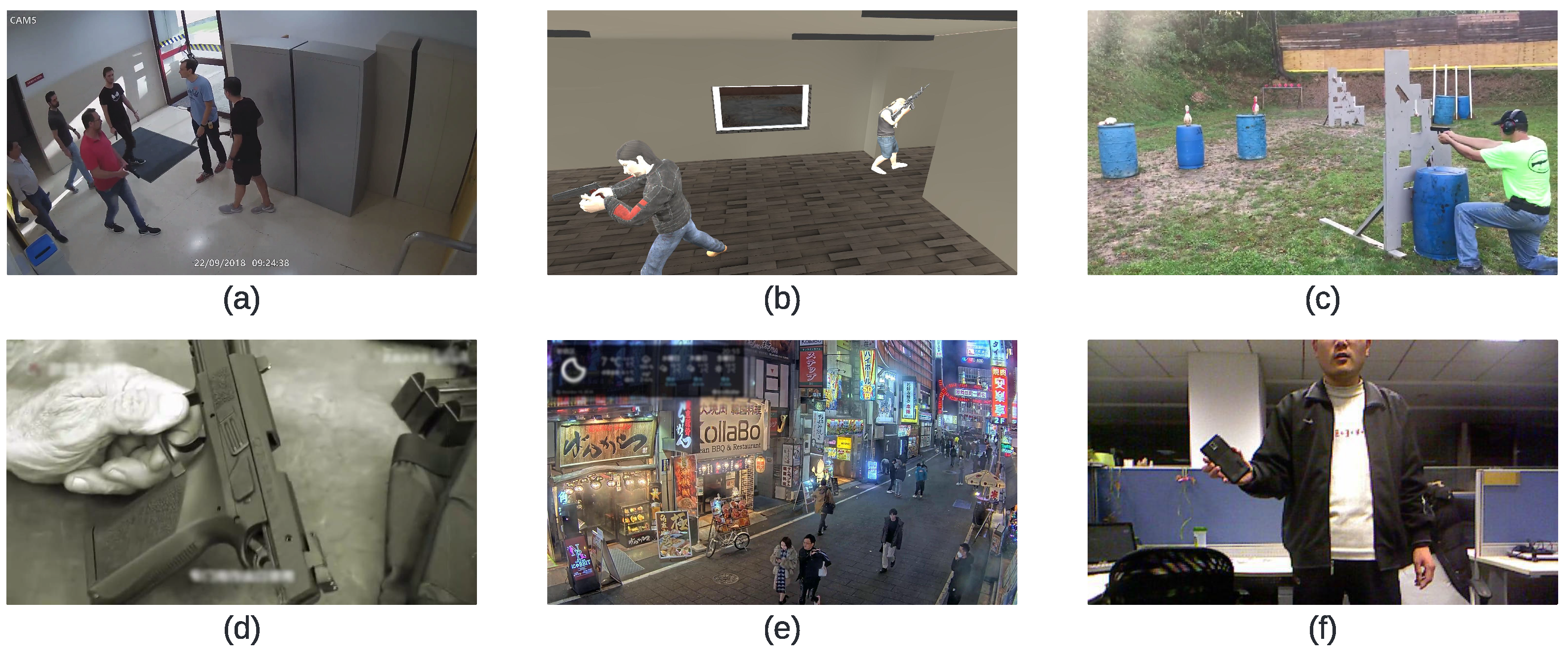
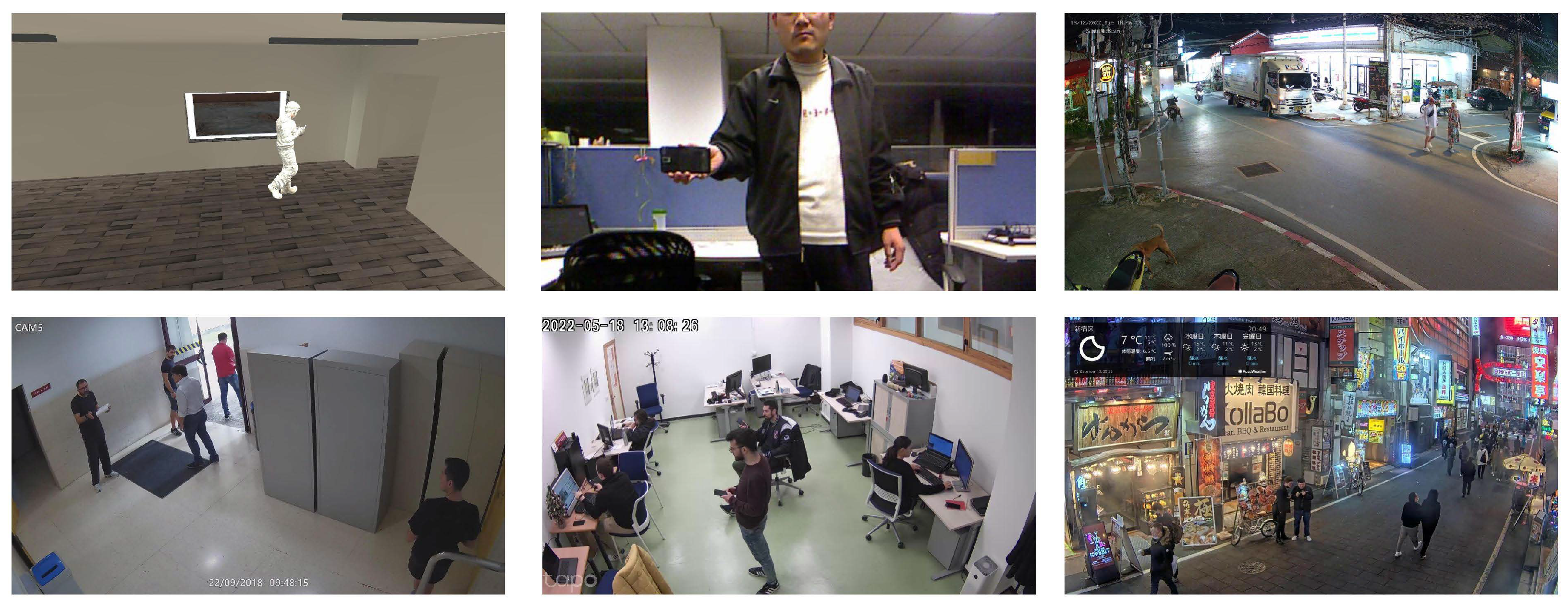
- usdataset [1]. This dataset was created at the University of Seville, capturing a simulated attack through a CCTV system. It encompasses two different scenarios; both cam 1 and cam 7 are directed towards a corridor with a door on one side and two exits in the background, experiencing minimal lighting variations, as they are indoors. Cam 5 is focused on an entrance, introducing ambient lighting and resulting in some lighting variations. The dataset comprises a total of 5149 images at 1080 p resolution, featuring 1520 instances of guns.
- usdataset_Synth [1]. This dataset is generated through simulation using the Unity engine. Gun annotations were performed automatically by the engine, yielding a substantial number of annotated images without the need for human annotation. The dataset is presented in three versions based on the number of images included: U0.5, U1.0, and U2.5 (500, 1000, 2500, respectively).
- Gun-Dataset [3]. This dataset consists of over 51,889 labelled images containing weapons. For our purposes, we use 46,242 labelled images, with the majority of weapons positioned in the foreground.
- YouTube-GDD [4]. This dataset comprises images extracted from YouTube videos. It includes two classes, gun and person, but our experiments focus solely on the gun class. The dataset comprises 5000 images at a resolution of 720 p, featuring 16,064 instances of weapons.
- HOD-Dataset [5]. Utilised to provide the detector with background images of objects that may resemble weapons, this dataset includes over 12,800 images of handheld objects. In our case, only five classes from the original dataset are used: mobile phone, keyboard, calculator, cup, mobile HDD, resulting in a total of 4200 images.
3.2. Weapon Detector
3.3. Scale Match
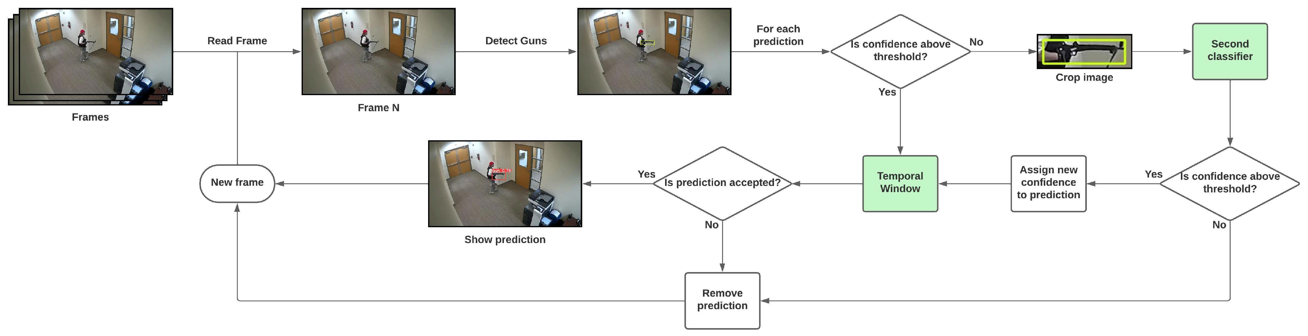
3.4. Detection Scheme
3.4.1. Secondary Classifier
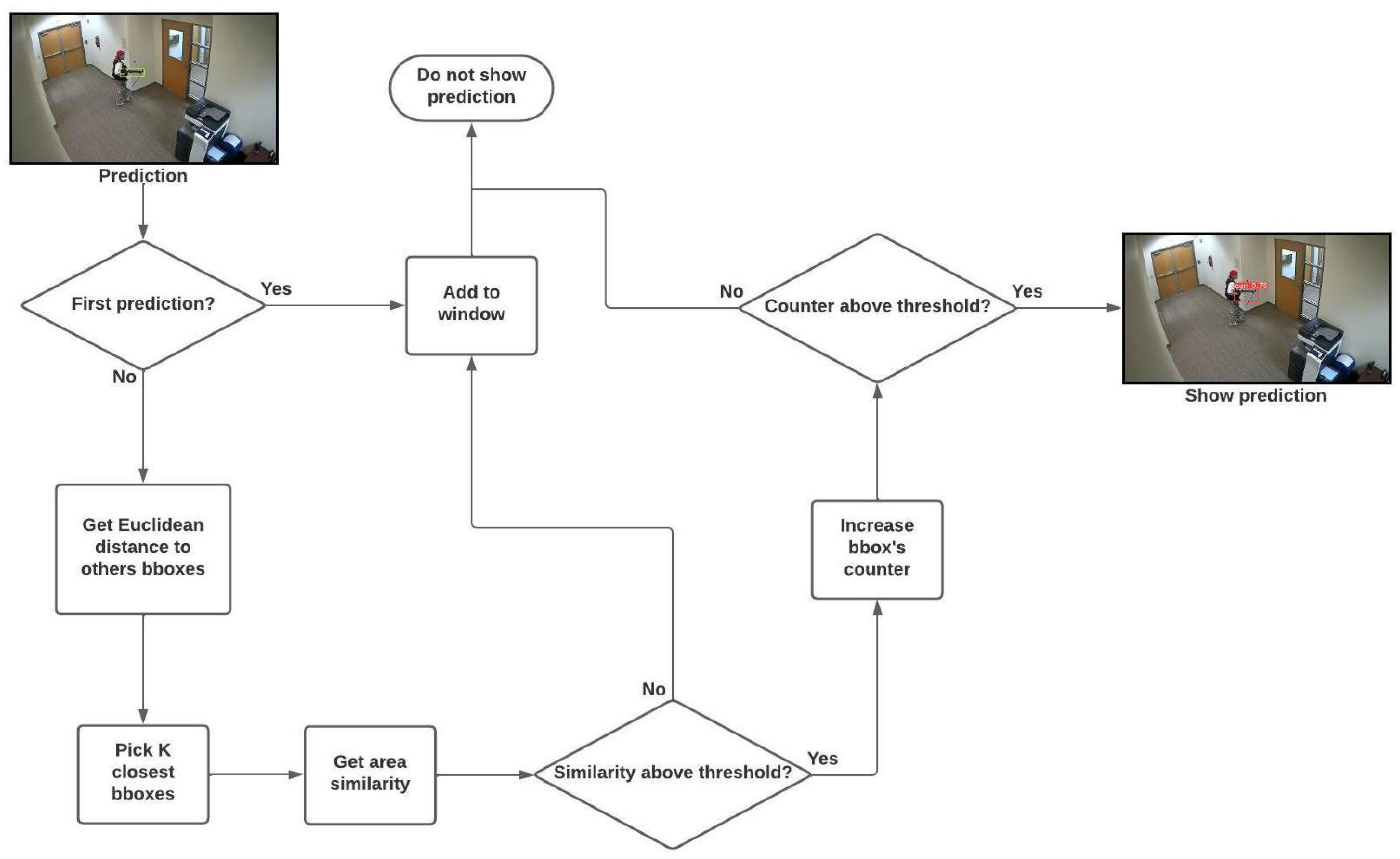
3.4.2. Temporal Window
4. Results
- The performance of various models and their different sizes will be studied from numerous training datasets. Additionally, the improvement of adding diverse amounts of background images in the best dataset will be tested.
- The impact on performance will be evaluated, in terms of accuracy, when using varying data augmentations and the two versions of Scale Match during training.
- Finally, the study will evaluate the performance and efficacy in accuracy and inference time of using the two proposed modules in the detection scheme on the best model obtained.
4.1. First Phase
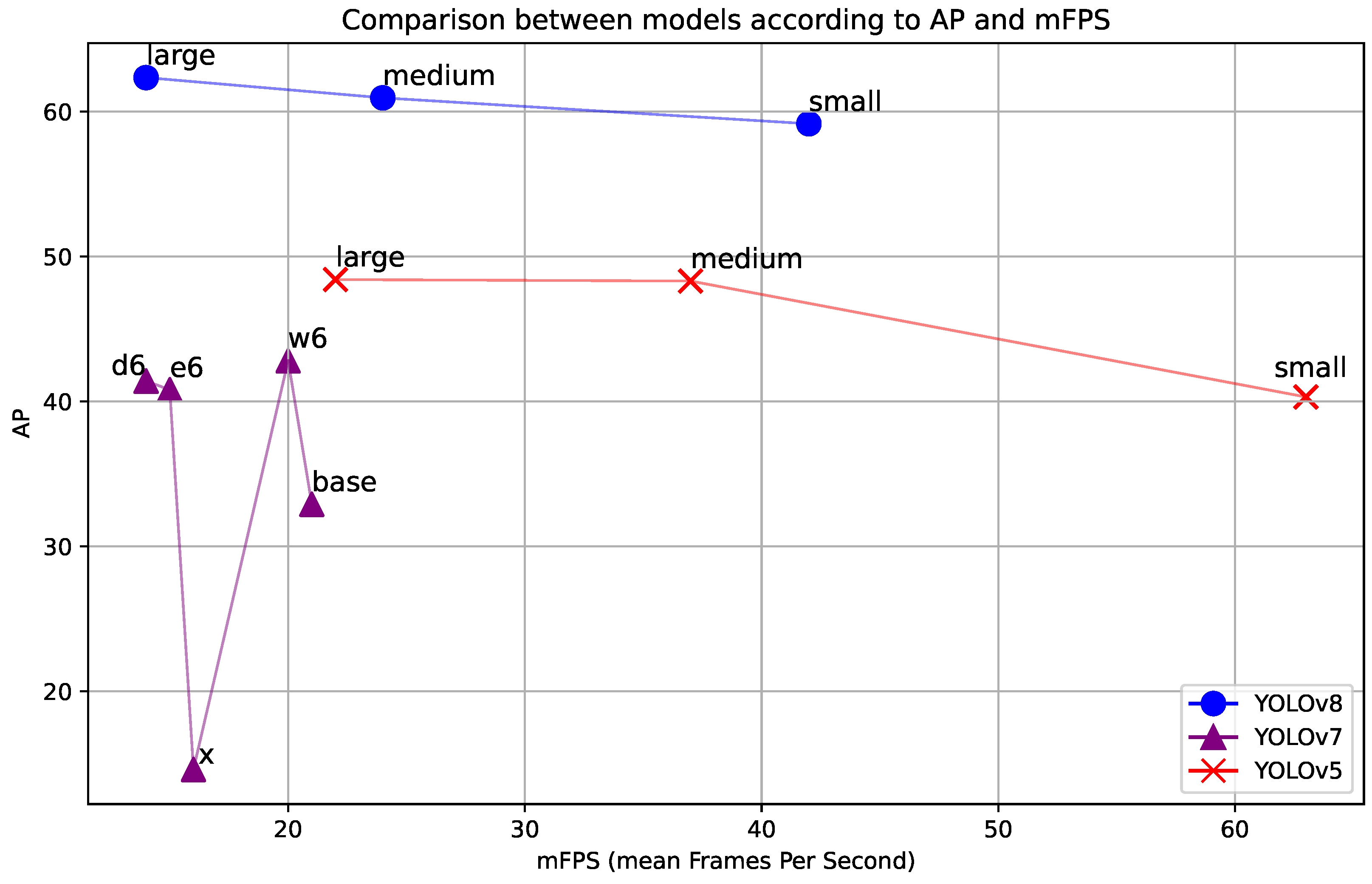
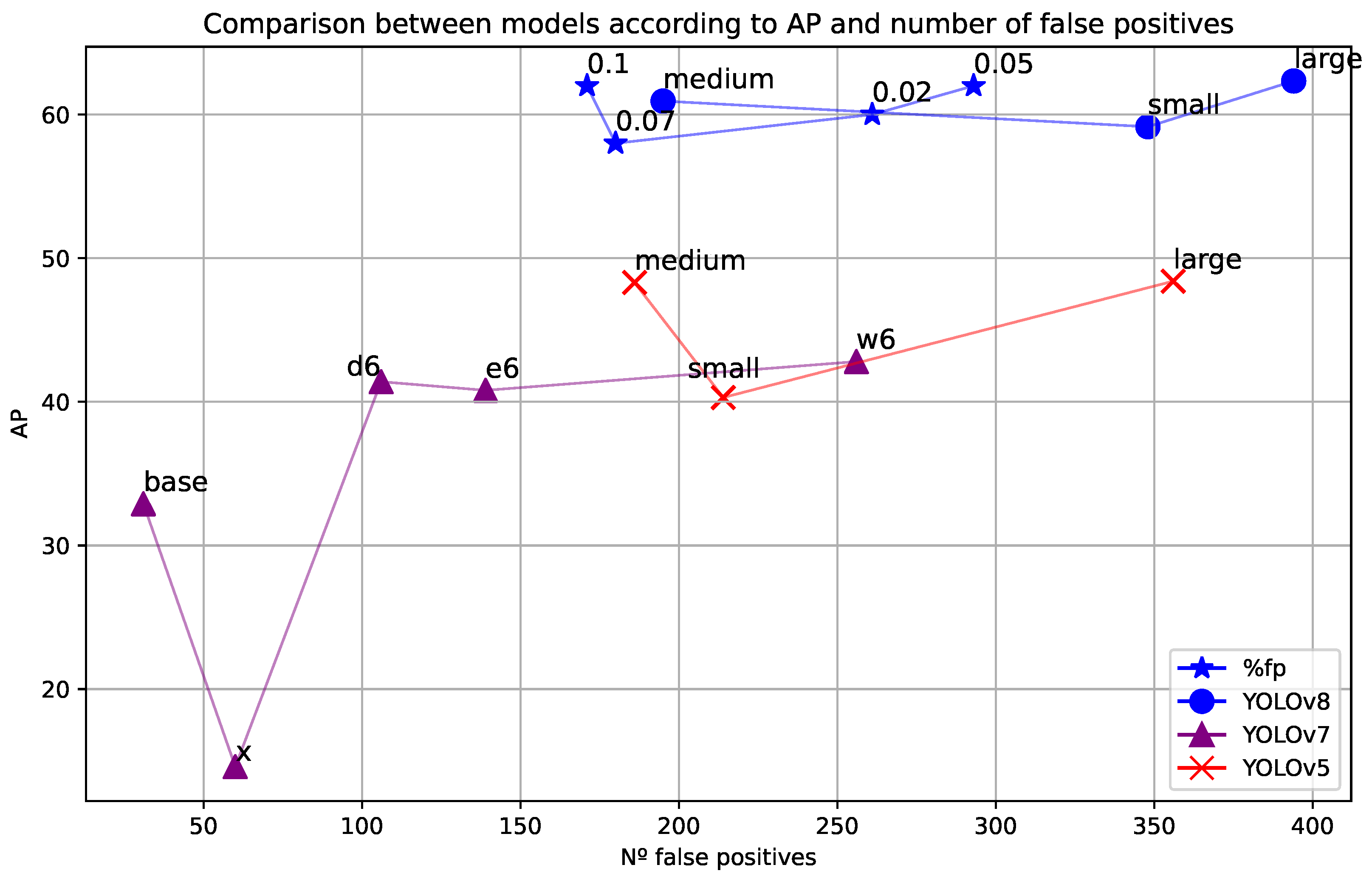
4.1.1. Models
4.1.2. Background Images
4.2. Second Phase
4.2.1. Data-Augmentation
- Blur: applies a blur with a maximum size of 10 × 10 pixels to the image with a probability of 50%.
- Cutout: applies three black squares, each 10% of the size of the image, with a probability of 50%.
- Horizontal Flip: applies a horizontal flip with a probability of 50%.
- Color Augmentation: applies different Hue, Saturation, and Value variations with a probability of 50% (0.015, 0.7, 0.4, respectively).
- ISONoise: applies a camera noise to the image with a probability of 50%, a colour variance of between 0.05 and 0.4, and an intensity of between 0.1 and 0.7.
- Random Brightness applies random image lighting variations with a probability of 50%.
- Rotate applies rotation with a probability of 50% and a range from −15° to 15°.
- Translate applies translation of the image with a gain of .
4.2.2. Scale Match
4.3. Third Phase
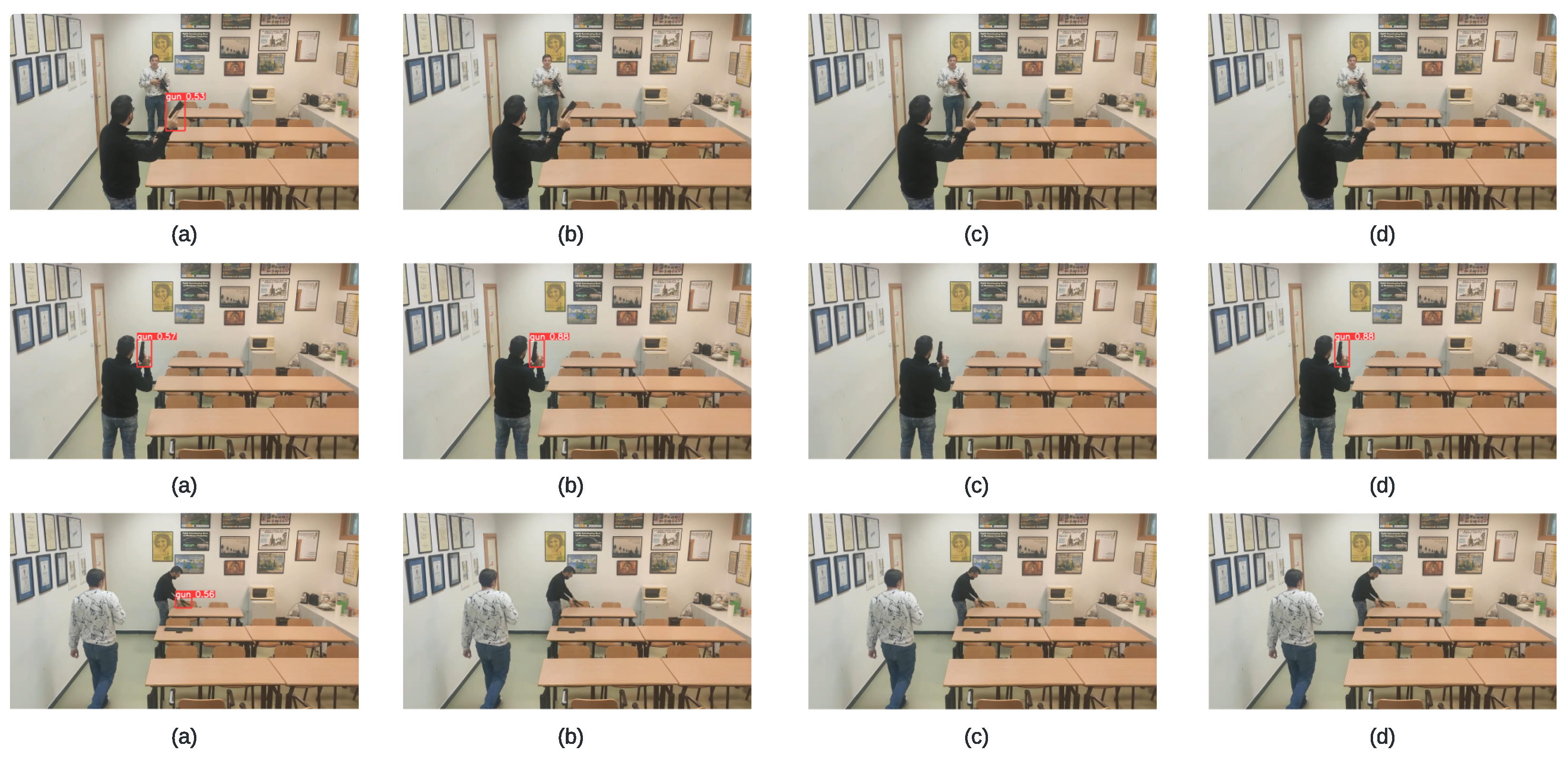
4.3.1. Detection Scheme’s Modules
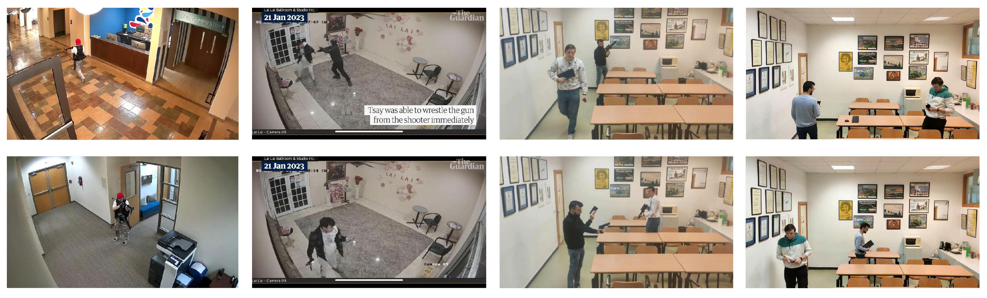
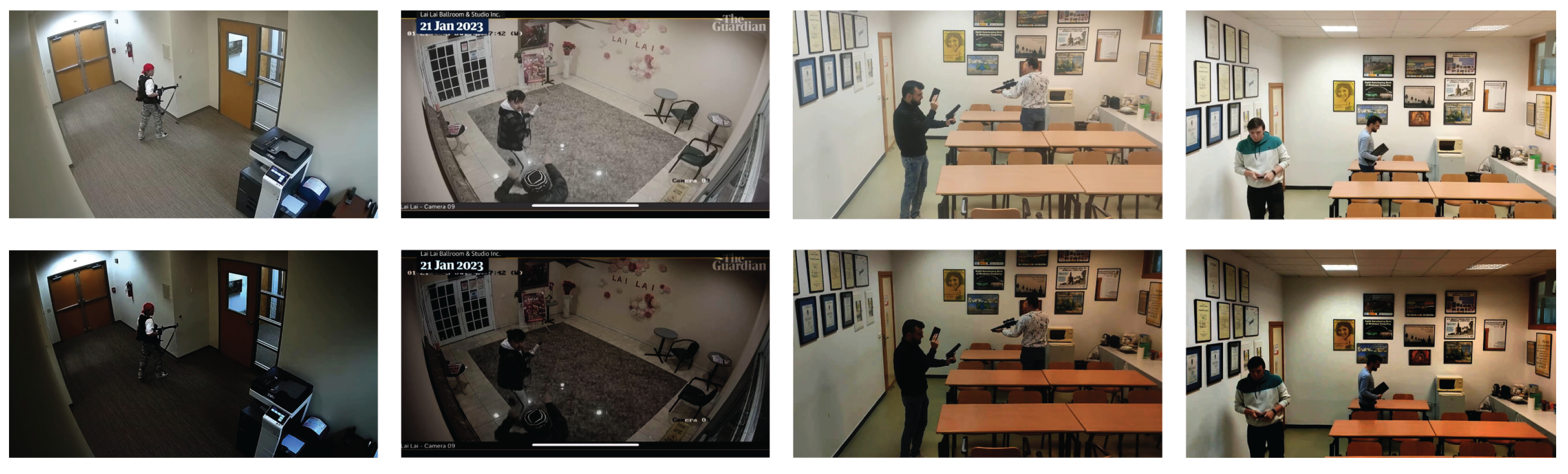
4.3.2. Detection Scheme’s Effectiveness on Darker Scenes
4.3.3. Comparison on Different Combinations
5. Discussion
6. Conclusions
Author Contributions
Funding
Institutional Review Board Statement
Informed Consent Statement
Data Availability Statement
Acknowledgments
Conflicts of Interest
References
- González, J.L.S.; Zaccaro, C.; Álvarez García, J.A.; Morillo, L.M.S.; Caparrini, F.S. Real-time gun detection in CCTV: An open problem. Neural Netw. 2020, 132, 297–308. [Google Scholar] [CrossRef]
- Velastin, S.A.; Boghossian, B.A.; Vicencio-Silva, M.A. A motion-based image processing system for detecting potentially dangerous situations in underground railway stations. Transp. Res. Part C Emerg. Technol. 2006, 14, 96–113. [Google Scholar] [CrossRef]
- Qi, D.; Tan, W.; Liu, Z.; Yao, Q.; Liu, J. A Dataset and System for Real-Time Gun Detection in Surveillance Video Using Deep Learning. In Proceedings of the 2021 IEEE International Conference on Systems, Man, and Cybernetics (SMC), Melbourne, Australia, 17–20 October 2021; pp. 667–672. [Google Scholar] [CrossRef]
- Gu, Y.; Liao, X.; Qin, X. YouTube-GDD: A challenging gun detection dataset with rich contextual information. arXiv 2022, arXiv:2203.04129. [Google Scholar]
- Qiao, L.; Li, X.; Jiang, S. RGB-D Object Recognition from Hand-Held Object Teaching. In Proceedings of the International Conference on Internet Multimedia Computing and Service, ICIMCS’16, Xi’an, China, 19–21 August 2016; pp. 31–34. [Google Scholar] [CrossRef]
- Olmos, R.; Tabik, S.; Herrera, F. Automatic handgun detection alarm in videos using deep learning. Neurocomputing 2018, 275, 66–72. [Google Scholar] [CrossRef]
- Olmos, R.; Tabik, S.; Lamas, A.; Pérez-Hernández, F.; Herrera, F. A binocular image fusion approach for minimizing false positives in handgun detection with deep learning. Inf. Fusion 2019, 49, 271–280. [Google Scholar] [CrossRef]
- Romero, D.; Salamea, C. Convolutional models for the detection of firearms in surveillance videos. Appl. Sci. 2019, 9, 2965. [Google Scholar] [CrossRef]
- Redmon, J.; Divvala, S.; Girshick, R.; Farhadi, A. You Only Look Once: Unified, Real-Time Object Detection. In Proceedings of the IEEE Conference on Computer Vision and Pattern Recognition (CVPR), Las Vegas, NV, USA, 27–30 June 2016; pp. 779–788. [Google Scholar] [CrossRef]
- Pang, L.; Liu, H.; Chen, Y.; Miao, J. Real-time concealed object detection from passive millimeter wave images based on the YOLOv3 algorithm. Sensors 2020, 20, 1678. [Google Scholar] [CrossRef]
- Wang, G.; Ding, H.; Duan, M.; Pu, Y.; Yang, Z.; Li, H. Fighting against terrorism: A real-time CCTV autonomous weapons detection based on improved YOLO v4. Digit. Signal Process. 2023, 132, 103790. [Google Scholar] [CrossRef]
- Ahmed, S.; Bhatti, M.T.; Khan, M.G.; Lövström, B.; Shahid, M. Development and Optimization of Deep Learning Models for Weapon Detection in Surveillance Videos. Appl. Sci. 2022, 12, 5772. [Google Scholar] [CrossRef]
- Castillo, A.; Tabik, S.; Pérez, F.; Olmos, R.; Herrera, F. Brightness guided preprocessing for automatic cold steel weapon detection in surveillance videos with deep learning. Neurocomputing 2019, 330, 151–161. [Google Scholar] [CrossRef]
- Pérez-Hernández, F.; Tabik, S.; Lamas, A.; Olmos, R.; Fujita, H.; Herrera, F. Object Detection Binary Classifiers methodology based on deep learning to identify small objects handled similarly: Application in video surveillance. Knowl.-Based Syst. 2020, 194, 105590. [Google Scholar] [CrossRef]
- Salido, J.; Lomas, V.; Ruiz-Santaquiteria, J.; Deniz, O. Automatic Handgun Detection with Deep Learning in Video Surveillance Images. Appl. Sci. 2021, 11, 6085. [Google Scholar] [CrossRef]
- Ashraf, A.H.; Imran, M.; Qahtani, A.M.; Alsufyani, A.; Almutiry, O.; Mahmood, A.; Attique, M.; Habib, M. Weapons detection for security and video surveillance using cnn and YOLO-v5s. CMC-Comput. Mater. Contin. 2022, 70, 2761–2775. [Google Scholar] [CrossRef]
- Goenka, A.; Sitara, K. Weapon Detection from Surveillance Images using Deep Learning. In Proceedings of the 2022 3rd International Conference for Emerging Technology (INCET), Belgaum, India, 27–29 May 2022; pp. 1–6. [Google Scholar] [CrossRef]
- Perea-Trigo, M.; López-Ortiz, E.J.; Salazar-González, J.L.; Álvarez-García, J.A.; Vegas Olmos, J.J. Data Processing Unit for Energy Saving in Computer Vision: Weapon Detection Use Case. Electronics 2022, 12, 146. [Google Scholar] [CrossRef]
- Hnoohom, N.; Chotivatunyu, P.; Jitpattanakul, A. ACF: An armed CCTV footage dataset for enhancing weapon detection. Sensors 2022, 22, 7158. [Google Scholar] [CrossRef]
- Berardini, D.; Migliorelli, L.; Galdelli, A.; Frontoni, E.; Mancini, A.; Moccia, S. A deep-learning framework running on edge devices for handgun and knife detection from indoor video-surveillance cameras. Multimed. Tools Appl. 2023, 83, 19109–19127. [Google Scholar] [CrossRef]
- Lin, T.Y.; Maire, M.; Belongie, S.; Hays, J.; Perona, P.; Ramanan, D.; Dollár, P.; Zitnick, C.L. Microsoft coco: Common objects in context. In Proceedings of the Computer Vision–ECCV 2014: 13th European Conference, Zurich, Switzerland, 6–12 September 2014; Proceedings, Part V 13. Springer: Berlin/Heidelberg, Germany, 2014; pp. 740–755. [Google Scholar] [CrossRef]
- Arcos-García, Á.; Álvarez García, J.A.; Soria-Morillo, L.M. Deep neural network for traffic sign recognition systems: An analysis of spatial transformers and stochastic optimisation methods. Neural Netw. 2018, 99, 158–165. [Google Scholar] [CrossRef]
- Arcos-García, Á.; Álvarez García, J.A.; Soria-Morillo, L.M. Evaluation of deep neural networks for traffic sign detection systems. Neurocomputing 2018, 316, 332–344. [Google Scholar] [CrossRef]
- Yu, X.; Han, Z.; Gong, Y.; Jan, N.; Zhao, J.; Ye, Q.; Chen, J.; Feng, Y.; Zhang, B.; Wang, X.; et al. The 1st tiny object detection challenge: Methods and results. In Proceedings of the Computer Vision–ECCV 2020 Workshops, Glasgow, UK, 23–28 August 2020; Proceedings, Part V 16. Springer: Berlin/Heidelberg, Germany, 2020; pp. 315–323. [Google Scholar] [CrossRef]
- Li, J.; Liang, X.; Wei, Y.; Xu, T.; Feng, J.; Yan, S. Perceptual generative adversarial networks for small object detection. In Proceedings of the IEEE Conference on Computer Vision and Pattern Recognition, Honolulu, HI, USA, 21–26 July 2017; pp. 1222–1230. [Google Scholar] [CrossRef]
- Hong, M.; Li, S.; Yang, Y.; Zhu, F.; Zhao, Q.; Lu, L. SSPNet: Scale Selection Pyramid Network for Tiny Person Detection From UAV Images. IEEE Geosci. Remote Sens. Lett. 2022, 19, 1–5. [Google Scholar] [CrossRef]
- Yu, X.; Gong, Y.; Jiang, N.; Ye, Q.; Han, Z. Scale Match for Tiny Person Detection. In Proceedings of the 2020 IEEE Winter Conference on Applications of Computer Vision (WACV), Snowmass Village, CO, USA, 1–5 March 2020; pp. 1246–1254. [Google Scholar] [CrossRef]
- Zhang, W.; Wang, S.; Thachan, S.; Chen, J.; Qian, Y. Deconv R-CNN for Small Object Detection on Remote Sensing Images. In Proceedings of the IGARSS 2018—2018 IEEE International Geoscience and Remote Sensing Symposium, Valencia, Spain, 22–27 July 2018; pp. 2483–2486. [Google Scholar] [CrossRef]
- Lin, T.Y.; Dollár, P.; Girshick, R.; He, K.; Hariharan, B.; Belongie, S. Feature pyramid networks for object detection. In Proceedings of the IEEE Conference on Computer Vision and Pattern Recognition, Honolulu, HI, USA, 21–26 July 2017; pp. 2117–2125. [Google Scholar] [CrossRef]
- Li, R.; Yang, J. Improved YOLOv2 object detection model. In Proceedings of the 2018 6th International Conference on Multimedia Computing and Systems (ICMCS), Rabat, Morocco, 10–12 May 2018; pp. 1–6. [Google Scholar] [CrossRef]
- Liang, Z.; Shao, J.; Zhang, D.; Gao, L. Small object detection using deep feature pyramid networks. In Proceedings of the Advances in Multimedia Information Processing–PCM 2018: 19th Pacific-Rim Conference on Multimedia, Hefei, China, 21–22 September 2018; Proceedings, Part III 19. Springer: Berlin/Heidelberg, Germany, 2018; pp. 554–564. [Google Scholar] [CrossRef]
- Li, W.; Zhang, L.; Wu, C.; Cui, Z.; Niu, C. A new lightweight deep neural network for surface scratch detection. Int. J. Adv. Manuf. Technol. 2022, 123, 1999–2015. [Google Scholar] [CrossRef]
- Liu, W.; Anguelov, D.; Erhan, D.; Szegedy, C.; Reed, S.; Fu, C.Y.; Berg, A.C. Ssd: Single shot multibox detector. In Proceedings of the Computer Vision–ECCV 2016: 14th European Conference, Amsterdam, The Netherlands, 11–14 October 2016; Proceedings, Part I 14. Springer: Berlin/Heidelberg, Germany, 2016; pp. 21–37. [Google Scholar] [CrossRef]
- Redmon, J.; Farhadi, A. YOLO9000: Better, Faster, Stronger. In Proceedings of the 2017 IEEE Conference on Computer Vision and Pattern Recognition (CVPR), Honolulu, HI, USA, 21–26 July 2017; pp. 6517–6525. [Google Scholar] [CrossRef]
- Redmon, J.; Farhadi, A. Yolov3: An incremental improvement. arXiv 2018, arXiv:1804.02767. [Google Scholar]
- Bochkovskiy, A.; Wang, C.Y.; Liao, H.Y.M. Yolov4: Optimal speed and accuracy of object detection. arXiv 2020, arXiv:2004.10934. [Google Scholar]
- Jocher, G. Ultralytics YOLOv5. Available online: https://github.com/ultralytics/yolov5 (accessed on 7 March 2024).
- Li, C.; Li, L.; Geng, Y.; Jiang, H.; Cheng, M.; Zhang, B.; Ke, Z.; Xu, X.; Chu, X. Yolov6 v3. 0: A full-scale reloading. arXiv 2023, arXiv:2301.05586. [Google Scholar]
- Wang, C.Y.; Bochkovskiy, A.; Liao, H.Y.M. YOLOv7: Trainable bag-of-freebies sets new state-of-the-art for real-time object detectors. arXiv 2022, arXiv:2207.02696. [Google Scholar]
- Jocher, G.; Chaurasia, A.; Qiu, J. YOLO by Ultralytics. Available online: https://github.com/ultralytics/ultralytics (accessed on 4 May 2024).
- Lu, S.; Wang, B.; Wang, H.; Chen, L.; Linjian, M.; Zhang, X. A real-time object detection algorithm for video. Comput. Electr. Eng. 2019, 77, 398–408. [Google Scholar] [CrossRef]
- Huang, R.; Pedoeem, J.; Chen, C. YOLO-LITE: A Real-Time Object Detection Algorithm Optimized for Non-GPU Computers. In Proceedings of the 2018 IEEE International Conference on Big Data (Big Data), Seattle, WA, USA, 10–13 December 2018; pp. 2503–2510. [Google Scholar] [CrossRef]
- Gupta, C.; Gill, N.S.; Gulia, P.; Chatterjee, J.M. A novel finetuned YOLOv6 transfer learning model for real-time object detection. J. Real-Time Image Process. 2023, 20, 42. [Google Scholar] [CrossRef]
- Xia, R.; Li, G.; Huang, Z.; Meng, H.; Pang, Y. Bi-path combination YOLO for real-time few-shot object detection. Pattern Recognit. Lett. 2023, 165, 91–97. [Google Scholar] [CrossRef]
- Sun, W.; Dai, L.; Zhang, X.; Chang, P.; He, X. RSOD: Real-time small object detection algorithm in UAV-based traffic monitoring. Appl. Intell. 2021, 52, 8448–8463. [Google Scholar] [CrossRef]
- Fang, W.; Wang, L.; Ren, P. Tinier-YOLO: A Real-Time Object Detection Method for Constrained Environments. IEEE Access 2020, 8, 1935–1944. [Google Scholar] [CrossRef]
- Wang, C.Y.; Bochkovskiy, A.; Liao, H.Y.M. Scaled-YOLOv4: Scaling Cross Stage Partial Network. In Proceedings of the 2021 IEEE/CVF Conference on Computer Vision and Pattern Recognition (CVPR), Nashville, TN, USA, 20–25 June 2021; pp. 13024–13033. [Google Scholar] [CrossRef]
- Ganesh, P.; Chen, Y.; Yang, Y.; Chen, D.; Winslett, M. YOLO-ReT: Towards High Accuracy Real-time Object Detection on Edge GPUs. In Proceedings of the 2022 IEEE/CVF Winter Conference on Applications of Computer Vision (WACV), Waikoloa, HI, USA, 3–8 January 2022; pp. 1311–1321. [Google Scholar] [CrossRef]
- Wang, T.; Anwer, R.M.; Cholakkal, H.; Khan, F.S.; Pang, Y.; Shao, L. Learning Rich Features at High-Speed for Single-Shot Object Detection. In Proceedings of the 2019 IEEE/CVF International Conference on Computer Vision (ICCV), Seoul, Republic of Korea, 27 October–2 November 2019; pp. 1971–1980. [Google Scholar] [CrossRef]
- Wang, R.J.; Li, X.; Ling, C.X. Pelee: A Real-Time Object Detection System on Mobile Devices. In Proceedings of the 32nd International Conference on Neural Information Processing Systems, NIPS’18, Montreal, QC, Canada, 3–8 December 2018; pp. 1967–1976. [Google Scholar]
- Lee, Y.; Hwang, J.w.; Lee, S.; Bae, Y.; Park, J. An Energy and GPU-Computation Efficient Backbone Network for Real-Time Object Detection. In Proceedings of the 2019 IEEE/CVF Conference on Computer Vision and Pattern Recognition Workshops (CVPRW), Long Beach, CA, USA, 16–17 June 2019; pp. 752–760. [Google Scholar] [CrossRef]
- Law, H.; Teng, Y.; Russakovsky, O.; Deng, J. Cornernet-lite: Efficient keypoint based object detection. arXiv 2019, arXiv:1904.08900. [Google Scholar]
- Qin, Z.; Li, Z.; Zhang, Z.; Bao, Y.; Yu, G.; Peng, Y.; Sun, J. ThunderNet: Towards real-time generic object detection on mobile devices. In Proceedings of the IEEE/CVF International Conference on Computer Vision, Seoul, Republic of Korea, 27 October–2 November 2019; pp. 6718–6727. [Google Scholar] [CrossRef]
- Shih, K.H.; Chiu, C.T.; Lin, J.A.; Bu, Y.Y. Real-Time Object Detection With Reduced Region Proposal Network via Multi-Feature Concatenation. IEEE Trans. Neural Netw. Learn. Syst. 2020, 31, 2164–2173. [Google Scholar] [CrossRef] [PubMed]
- Dosovitskiy, A.; Beyer, L.; Kolesnikov, A.; Weissenborn, D.; Zhai, X.; Unterthiner, T.; Dehghani, M.; Minderer, M.; Heigold, G.; Gelly, S.; et al. An image is worth 16x16 words: Transformers for image recognition at scale. arXiv 2020, arXiv:2010.11929. [Google Scholar]
- Carion, N.; Massa, F.; Synnaeve, G.; Usunier, N.; Kirillov, A.; Zagoruyko, S. End-to-End Object Detection with Transformers. In Proceedings of the Computer Vision—ECCV 2020, Glasgow, UK, 23–28 August 2020; pp. 213–229. [Google Scholar] [CrossRef]
- Liu, Z.; Lin, Y.; Cao, Y.; Hu, H.; Wei, Y.; Zhang, Z.; Lin, S.; Guo, B. Swin Transformer: Hierarchical Vision Transformer using Shifted Windows. In Proceedings of the 2021 IEEE/CVF International Conference on Computer Vision (ICCV), Montreal, QC, Canada, 10–17 October 2021; pp. 9992–10002. [Google Scholar] [CrossRef]
- Wang, C.Y.; Mark Liao, H.Y.; Wu, Y.H.; Chen, P.Y.; Hsieh, J.W.; Yeh, I.H. CSPNet: A New Backbone that can Enhance Learning Capability of CNN. In Proceedings of the 2020 IEEE/CVF Conference on Computer Vision and Pattern Recognition Workshops (CVPRW), Seattle, WA, USA, 14–19 June 2020; pp. 1571–1580. [Google Scholar] [CrossRef]
- Tan, M.; Pang, R.; Le, Q.V. EfficientDet: Scalable and Efficient Object Detection. In Proceedings of the 2020 IEEE/CVF Conference on Computer Vision and Pattern Recognition (CVPR), Seattle, WA, USA, 13–19 June 2020; pp. 10778–10787. [Google Scholar] [CrossRef]
- Tan, M.; Le, Q. Efficientnet: Rethinking model scaling for convolutional neural networks. In Proceedings of the International Conference on Machine Learning, Long Beach, CA, USA, 9–15 June 2019; pp. 6105–6114. [Google Scholar]
- Sun, P.; Zhang, R.; Jiang, Y.; Kong, T.; Xu, C.; Zhan, W.; Tomizuka, M.; Li, L.; Yuan, Z.; Wang, C.; et al. Sparse r-cnn: End-to-end object detection with learnable proposals. In Proceedings of the IEEE/CVF Conference on Computer Vision and Pattern Recognition, Nashville, TN, USA, 20–25 June 2021; pp. 14454–14463. [Google Scholar] [CrossRef]
- Deng, J.; Dong, W.; Socher, R.; Li, L.J.; Li, K.; Fei-Fei, L. ImageNet: A large-scale hierarchical image database. In Proceedings of the 2009 IEEE Conference on Computer Vision and Pattern Recognition, Miami, FL, USA, 20–25 June 2009; pp. 248–255. [Google Scholar] [CrossRef]
- Yu, W.; Si, C.; Zhou, P.; Luo, M.; Zhou, Y.; Feng, J.; Yan, S.; Wang, X. Metaformer baselines for vision. arXiv 2022, arXiv:2210.13452. [Google Scholar] [CrossRef]
- Fang, Y.; Sun, Q.; Wang, X.; Huang, T.; Wang, X.; Cao, Y. Eva-02: A visual representation for neon genesis. arXiv 2023, arXiv:2303.11331. [Google Scholar] [CrossRef]
- Smith, L.N.; Topin, N. Super-convergence: Very fast training of neural networks using large learning rates. In Proceedings of the Artificial Intelligence and Machine Learning for Multi-Domain Operations Applications, Baltimore, MD, USA, 15–17 April 2019; Volume 11006, pp. 369–386. [Google Scholar] [CrossRef]


| Models | Dataset | Input Size | AP | mFPS |
|---|---|---|---|---|
| Salazar et al. [1] | usdataset + usdataset_Synth + UGR | - | 67.7 | - |
| Olmos et al. [6] | UGR | 1000 × 1000 | - | 5.3 |
| Wang et al. [11] | usdataset + usdataset_Synth + new images | 416 × 416 | 81.75 | 69.1 |
| Ashraf et al. [16] | Modified UGR | 416 × 416 | - | 25 |
| Hnoohom et al. [19] | ACF | 512 × 512 | 49.5 | 9 |
| Berardini et al. [20] | CCTV dataset | 416 × 416 | 79.30 | 5.10 |
| Ours | Disarm-Dataset | 1280 × 720 | 51.36 | 34 |
| Dataset | Class | No. of Images | No. of Instances | % of Low-Ambient-Light Images |
|---|---|---|---|---|
| usdataset | Gun | 1520 | 2511 | 0.0 |
| Others | 3629 | - | ||
| usdataset_Synth | Gun | 864 | 1110 | 0.0 |
| Others | 136 | - | ||
| usdataset_v2 | Gun | 1520 | 2511 | 0.0 |
| Others | 3629 | - | ||
| Gun-Dataset | Gun | 46,238 | 49,644 | 18.58 |
| Others | - | - | ||
| YouTube-GDD | Gun | 4500 | 7153 | 7.16 |
| Others | 500 | - | ||
| HOD-Dataset | Gun | - | - | 10.0 |
| Others | 1000 | - | ||
| FP-Dataset | Gun | - | - | 0.0 |
| Others | 36,000 | - | ||
| Disarm-Dataset | Gun | 60,081 | 64,994 | 14.58 |
| Others | 2650 | - |
| Model | Input Size | N° Parameters (M) | Inference Time (ms) |
|---|---|---|---|
| YOLOv5s | 640 | 7.2 | 6.4 |
| YOLOv5m | 640 | 21.2 | 8.2 |
| YOLOv5l | 640 | 46.5 | 10.1 |
| YOLOv5x | 640 | 86.7 | 12.1 |
| YOLOv7 | 640 | 36.9 | 6.21 |
| YOLOv7-X | 640 | 71.3 | 8.77 |
| YOLOv7-W6 | 1280 | 70.4 | 11.9 |
| YOLOv7-E6 | 1280 | 97.2 | 17.85 |
| YOLOv7-D6 | 1280 | 154.7 | 22.72 |
| YOLOv7-E6E | 1280 | 151.7 | 27.77 |
| YOLOv8n | 640 | 3.2 | 0.99 |
| YOLOv8s | 640 | 11.2 | 1.20 |
| YOLOv8m | 640 | 25.9 | 1.83 |
| YOLOv8l | 640 | 43.7 | 2.39 |
| YOLOv8x | 640 | 68.2 | 3.53 |
| Dataset | AP50 | AP75 | AP | F1 | FP |
|---|---|---|---|---|---|
| Disarm-Dataset | 42.80 | 50.90 | 42.80 | 69.70 | 196 |
| Gun-Dataset | 60.60 | 34.50 | 29.20 | 52.80 | 163 |
| YouTube-GDD | 0.50 | 0.30 | 0.20 | 0.00 | 2 |
| usdataset_v2 + synth | 0.70 | 0.70 | 0.60 | 0.40 | 0 |
| usdataset_v2 | 0.00 | 0.00 | 0.00 | 0.00 | 0 |
| usdataset + synth | 0.00 | 0.00 | 0.00 | 0.00 | 0 |
| usdataset | 0.00 | 0.00 | 0.00 | 0.00 | 0 |
| Model | AP50 | AP75 | AP | F1 | FP |
|---|---|---|---|---|---|
| YOLOv8l | 75.77 | 71.35 | 62.34 | 71.10 | 401 |
| YOLOv8m | 73.12 | 69.22 | 60.94 | 68.70 | 196 |
| YOLOv8s | 77.12 | 68.10 | 59.15 | 72.50 | 348 |
| YOLOv7-d6 | 59.00 | 47.00 | 41.40 | 72.00 | 106 |
| YOLOv7-e6 | 59.40 | 49.50 | 40.80 | 72.90 | 139 |
| YOLOv7-w6 | 59.80 | 50.90 | 42.80 | 72.80 | 256 |
| YOLOv7x | 19.90 | 18.90 | 14.60 | 58.00 | 60 |
| YOLOv7 | 40.10 | 38.80 | 32.90 | 56.60 | 31 |
| YOLOV5l | 66.50 | 58.80 | 48.40 | 61.40 | 356 |
| YOLOV5m | 67.60 | 58.10 | 48.30 | 61.90 | 186 |
| YOLOV5s | 59.70 | 48.60 | 40.30 | 49.00 | 214 |
| % BG Images | AP50 | AP75 | AP | F1 | FP |
|---|---|---|---|---|---|
| 10% | 76.35 | 71.90 | 61.99 | 71.60 | 171 |
| 7% | 74.22 | 67.51 | 58.37 | 68.30 | 180 |
| 5% | 77.21 | 73.18 | 62.81 | 72.50 | 293 |
| 2% | 74.30 | 69.83 | 60.24 | 68.90 | 261 |
| Baseline | 77.12 | 68.10 | 59.15 | 72.50 | 348 |
| Augment | AP50 | AP75 | AP | F1 | FP |
|---|---|---|---|---|---|
| no_blur_noise | 77.26 | 72.40 | 62.34 | 72.60 | 287 |
| no_blur_cutout | 77.35 | 72.30 | 62.69 | 73.20 | 245 |
| no_blur_bright | 76.13 | 71.80 | 61.26 | 71.60 | 117 |
| no_flip | 76.89 | 70.55 | 59.15 | 73.00 | 223 |
| no_blur | 77.23 | 73.06 | 62.77 | 73.10 | 202 |
| Default | 75.90 | 71.21 | 59.89 | 71.60 | 157 |
| Baseline | 77.21 | 73.18 | 62.81 | 72.50 | 293 |
| Area | Dataset | AP50 | AP75 | AP | F1 | FP |
|---|---|---|---|---|---|---|
| All | Scale Match paste | 70.00 | 58.18 | 48.10 | 66.70 | 408 |
| Scale Match | 77.68 | 73.88 | 63.41 | 73.60 | 164 | |
| Baseline | 77.23 | 73.06 | 62.77 | 73.10 | 202 | |
| ≤1002 | Scale Match paste | 41.26 | 30.46 | 26.09 | 47.01 | 407 |
| Scale Match | 62.33 | 53.46 | 46.30 | 65.15 | 164 | |
| Baseline | 49.10 | 42.55 | 36.39 | 54.43 | 199 |
| Combination | AP50 | AP75 | AP | F1 | FP | mFPS |
|---|---|---|---|---|---|---|
| All | 61.14 | 59.28 | 51.36 | 40.12 | 0 | 34 |
| + temp. wind. | 52.66 | 52.49 | 48.10 | 11.82 | 0 | 47 |
| + 2nd clas. | 75.72 | 71.31 | 61.09 | 71.71 | 48 | 34 |
| Baseline | 77.68 | 73.88 | 63.41 | 73.60 | 164 | 48 |
| Scenario | Combination | AP50 | AP75 | AP | F1 | FP | mFPS |
|---|---|---|---|---|---|---|---|
| Bright | All | 61.14 | 59.28 | 51.36 | 40.12 | 0 | 34 |
| + temp. wind. | 52.66 | 52.49 | 48.10 | 11.82 | 0 | 47 | |
| + 2nd clas. | 75.72 | 71.31 | 61.09 | 71.71 | 48 | 34 | |
| Baseline | 77.68 | 73.88 | 63.41 | 73.60 | 164 | 48 | |
| Dark | All | 58.95 | 55.37 | 46.33 | 37.77 | 0 | 34 |
| + temp. wind. | 50.75 | 50.19 | 44.36 | 10.04 | 0 | 47 | |
| + 2nd clas. | 73.10 | 66.08 | 54.90 | 67.16 | 32 | 34 | |
| Baseline | 74.11 | 67.99 | 56.73 | 65.45 | 84 | 48 |
| BG Images | Augs | S.M. | Temp. Wind. | 2nd Clas. | F1 | mAP50 | mAP75 | mAP | FP | |
|---|---|---|---|---|---|---|---|---|---|---|
| - | - | - | - | - | 77.12 | 68.10 | 59.15 | 72.50 | 348 | 347 |
| - | - | - | x | - | 53.29 | 52.05 | 46.48 | 17.47 | 0 | 0 |
| - | - | - | - | x | 75.29 | 64.95 | 56.06 | 71.06 | 90 | 90 |
| - | - | - | x | x | 62.67 | 55.90 | 48.80 | 45.81 | 0 | 0 |
| - | x | - | - | - | 76.97 | 72.52 | 62.48 | 73.65 | 205 | 205 |
| - | x | - | x | - | 53.11 | 52.94 | 46.84 | 11.71 | 0 | 0 |
| - | x | - | - | x | 74.60 | 69.46 | 59.63 | 72.20 | 51 | 51 |
| - | x | - | x | x | 58.74 | 55.06 | 47.73 | 38.55 | 0 | 0 |
| - | - | x | - | - | 77.95 | 72.76 | 64.58 | 74.05 | 317 | 315 |
| - | - | x | x | - | 55.65 | 54.01 | 49.46 | 24.54 | 0 | 0 |
| - | - | x | - | x | 75.99 | 70.62 | 62.16 | 73.27 | 96 | 96 |
| - | - | x | x | x | 62.92 | 59.51 | 52.99 | 46.33 | 1 | 1 |
| - | x | x | - | - | 77.08 | 71.91 | 63.54 | 73.42 | 334 | 333 |
| - | x | x | x | - | 58.78 | 56.86 | 51.37 | 34.90 | 0 | 0 |
| - | x | x | - | x | 75.72 | 69.71 | 61.40 | 73.17 | 108 | 108 |
| - | x | x | x | x | 68.89 | 65.56 | 57.83 | 58.05 | 0 | 0 |
| x | - | - | - | - | 77.21 | 73.18 | 62.81 | 72.50 | 293 | 289 |
| x | - | - | x | - | 54.61 | 53.87 | 47.50 | 19.28 | 0 | 0 |
| x | - | - | - | x | 75.69 | 71.07 | 60.49 | 71.61 | 90 | 90 |
| x | - | - | x | x | 65.14 | 61.99 | 53.02 | 50.02 | 0 | 0 |
| x | x | - | - | - | 77.23 | 73.06 | 62.77 | 73.10 | 202 | 199 |
| x | x | - | x | - | 54.62 | 53.35 | 47.81 | 19.10 | 0 | 0 |
| x | x | - | - | x | 76.42 | 71.87 | 61.33 | 72.56 | 87 | 87 |
| x | x | - | x | x | 58.52 | 56.90 | 49.53 | 34.07 | 0 | 0 |
| x | - | x | - | - | 77.64 | 72.91 | 64.83 | 73.99 | 445 | 444 |
| x | - | x | x | - | 56.42 | 54.85 | 50.19 | 28.85 | 0 | 0 |
| x | - | x | - | x | 75.85 | 70.46 | 62.39 | 72.89 | 64 | 64 |
| x | - | x | x | x | 65.93 | 62.31 | 55.89 | 54.81 | 0 | 0 |
| x | x | x | - | - | 77.68 | 73.88 | 63.41 | 73.60 | 164 | 164 |
| x | x | x | x | - | 52.66 | 52.49 | 48.10 | 11.82 | 0 | 0 |
| x | x | x | - | x | 75.72 | 71.31 | 61.09 | 71.71 | 48 | 48 |
| x | x | x | x | x | 61.14 | 59.28 | 51.36 | 40.12 | 0 | 0 |
Disclaimer/Publisher’s Note: The statements, opinions and data contained in all publications are solely those of the individual author(s) and contributor(s) and not of MDPI and/or the editor(s). MDPI and/or the editor(s) disclaim responsibility for any injury to people or property resulting from any ideas, methods, instructions or products referred to in the content. |
© 2024 by the authors. Licensee MDPI, Basel, Switzerland. This article is an open access article distributed under the terms and conditions of the Creative Commons Attribution (CC BY) license (https://creativecommons.org/licenses/by/4.0/).
Share and Cite
Torregrosa-Domínguez, Á.; Álvarez-García, J.A.; Salazar-González, J.L.; Soria-Morillo, L.M. Effective Strategies for Enhancing Real-Time Weapons Detection in Industry. Appl. Sci. 2024, 14, 8198. https://doi.org/10.3390/app14188198
Torregrosa-Domínguez Á, Álvarez-García JA, Salazar-González JL, Soria-Morillo LM. Effective Strategies for Enhancing Real-Time Weapons Detection in Industry. Applied Sciences. 2024; 14(18):8198. https://doi.org/10.3390/app14188198
Chicago/Turabian StyleTorregrosa-Domínguez, Ángel, Juan A. Álvarez-García, Jose L. Salazar-González, and Luis M. Soria-Morillo. 2024. "Effective Strategies for Enhancing Real-Time Weapons Detection in Industry" Applied Sciences 14, no. 18: 8198. https://doi.org/10.3390/app14188198