
Prediction of Ship-Unloading Time Using Neural Networks


Abstract
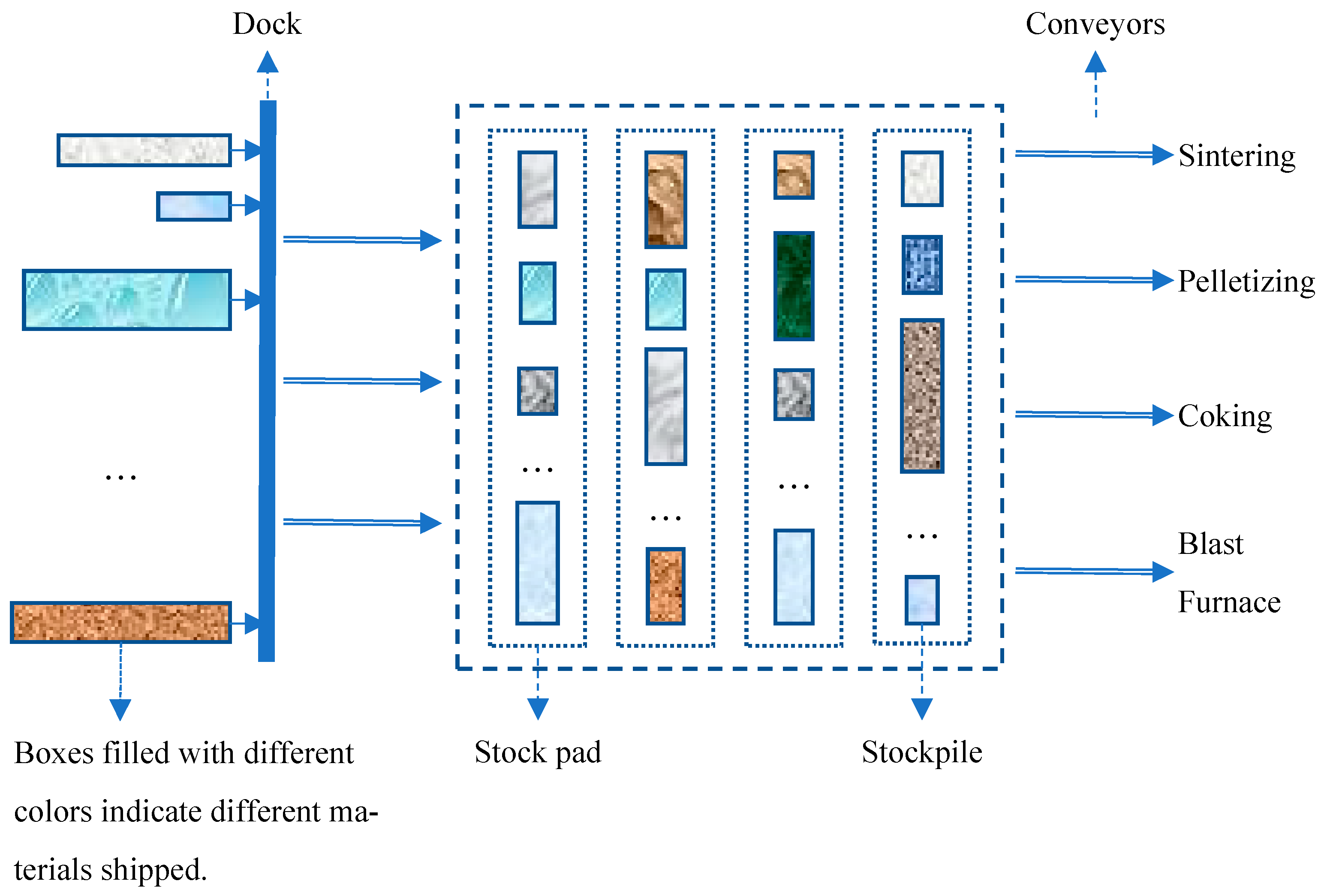
1. Introduction
- RVFL introduces an efficient way to find out the optimal network parameters and represents a richer structure variety of neural networks [19].
- SCN exhibits a concise network structure and demonstrates a better application potential [20].
- Three neural network models-Backpropagation (BP), Random Vector Functional Link (RVFL), and Stochastic Configuration (SCN) have been developed for predictive applications.
- Three prediction models are comprehensively evaluated based on their predictive accuracy, convergence, and stability, and are applied to a real-world scenario involving unloading-time prediction.
2. Literature Review
3. Related Methods
3.1. BP Neural Network
- Hidden layer outputs
- 2.
- Output layer results
- 3.
- Updating of weights
| Algorithm 1: BP algorithm |
| Input: samples {xi, yi}, xi ∈ Rd, yi ∈ Rl, i = 1, …, N; J Output: wij, wjk, i = 1, …, d; j=1, …, J; k = 1,…,l |
| Initialization: For all i, j wij = generateRandomNumber (−1, 1); //generate random numbers in interval [−1, 1]; For all j, k wjk = generateRandomNumber (−1, 1); //generate random numbers in interval [−1, 1]; η = 0.8; //learning rate Lmax = 5000; L = 0; ε = 0.001; //error bound While and , do 1. Calculate hidden layer outputs with Formula (1); 2. Calculate prediction values with Formula (2); 3. Calculate error: E = ; 4. Update weights with Formulas (3) and (4); 5. L++; End While Return wij, wjk; |
3.2. Random Vector Functional Link Network (RVFL)
| Algorithm 2: RVFL algorithm |
| Inputs: Input , and output , ; Bias ; The number of nodes in hidden layer ; the range of weights ; regularization parameter . Outputs: . 1: Initialize: randomly selecting the initial weights in range of , . , ; 2: Calculate activation values of the hidden layer: , where is an activation function 3: Establish enhancement layer to implement direct link: ; 4: Calculate output weights through regularized least squares method: 5: Return , there by can be calculated. |
3.3. Stochastic Configuration Networks
| Algorithm 3: SCN algorithm |
| Input: X = {x1, x2, …, xN }, xi ∈ Rd and outputs Y = {y1, y2, …, yN }, yi ∈ Rm; Lmax, ε, Tmax; Λ = {λmin: ∆λ: λmax}; Output: ,, |
| 1. Initialize e0: = [y1, y2, …, yN]T, 0 < r < 1, two empty sets Ω and W; 2. While L ≤ Lmax AND ‖e0‖ > ε, Do Phase 1: Stochastic parameters configuration (steps 3–17): 3. For λ ∈ Λ 4. For k = 1, 2, …, Tmax, Do 5. Randomly assign vL and bL from [−λ, λ]d and [−λ, λ], respectively; 6. Calculate gL, ξL,q based on Equations (17) and (19), and µL = (1 − r)/(L + 1); 7. If min {ξL,1, ξL,2, …, ξL,m} ≥ 0 8. Save wL and bL in W, in Ω, respectively; 9. Else go back to step 4; 10. End If 11. End For (corresponds to Step 4) 12. If W is not empty 13. Find wL*, bL* that maximize ξL in Ω, and set GL = [g1*, g2*, …, gL*]; 14. Break (go to step 18); 15. Else randomly take τ ∈ (0, 1 − r), renew r: = r + τ, return to step 4; 16. End If 17. End For (corresponds to step 3) Phase 2: Output weights computation: 18. Obtain GL = [g1*, g2*, …, gL*]; 19. Calculate β* = [β1*, β2*, …, βL*]T = GL+·Y; 20. Calculate eL = eL−1 − βL*gL*; 21. Renew e0: =eL; L: =L + 1; 22. End While 23. Return β1*, β2*, …, βL*, w* = [w1*, w2*, …, wL*], b = [b1*, b2*, …, bL*]. |
3.4. Evaluation Metrics
4. Experimental Results
- (1)
- DB1
- (2)
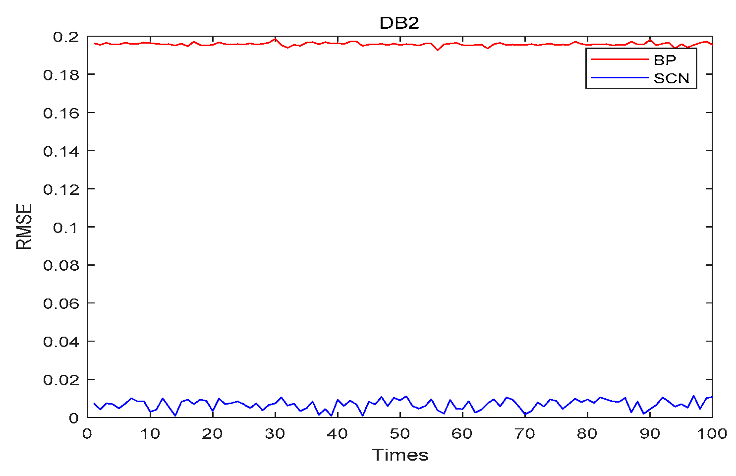
- DB2
- (3)
- DB3 (stock) is a standard dataset for regression prediction from the KEEL website. The data is the daily stock prices of 10 aerospace companies from January 1988 to October 1991. The task is to predict the price of the 10th company, given the prices of the rest of the companies.
- (4)
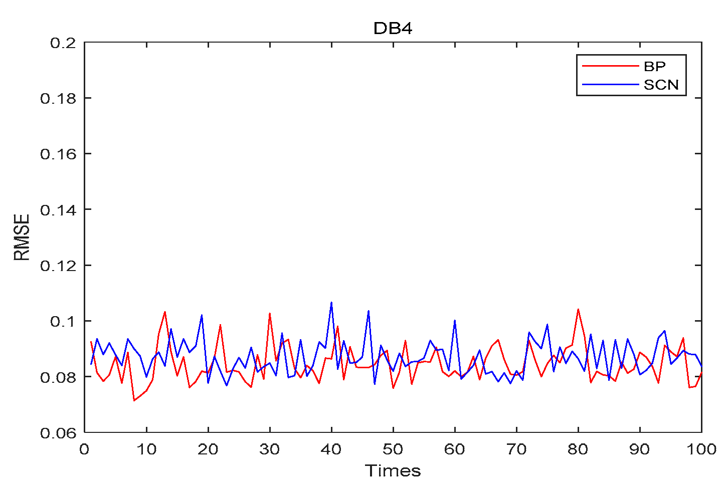
- DB4 (concrete) is a standard dataset for regression prediction from the KEEL website. The concrete compressive strength is a nonlinear function of age and ingredients. The task is to predict the concrete compressive strength.
4.1. Network Structure
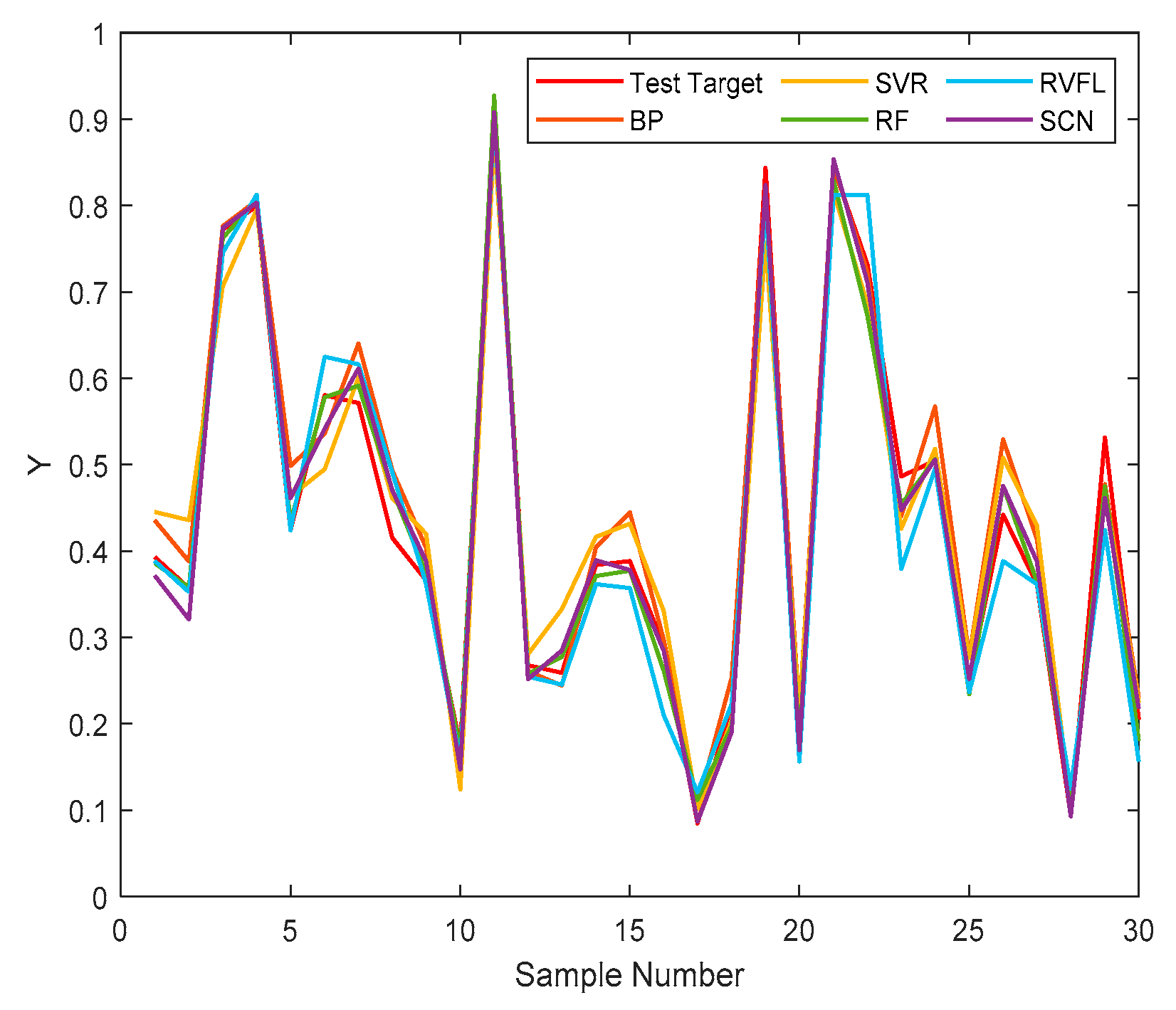
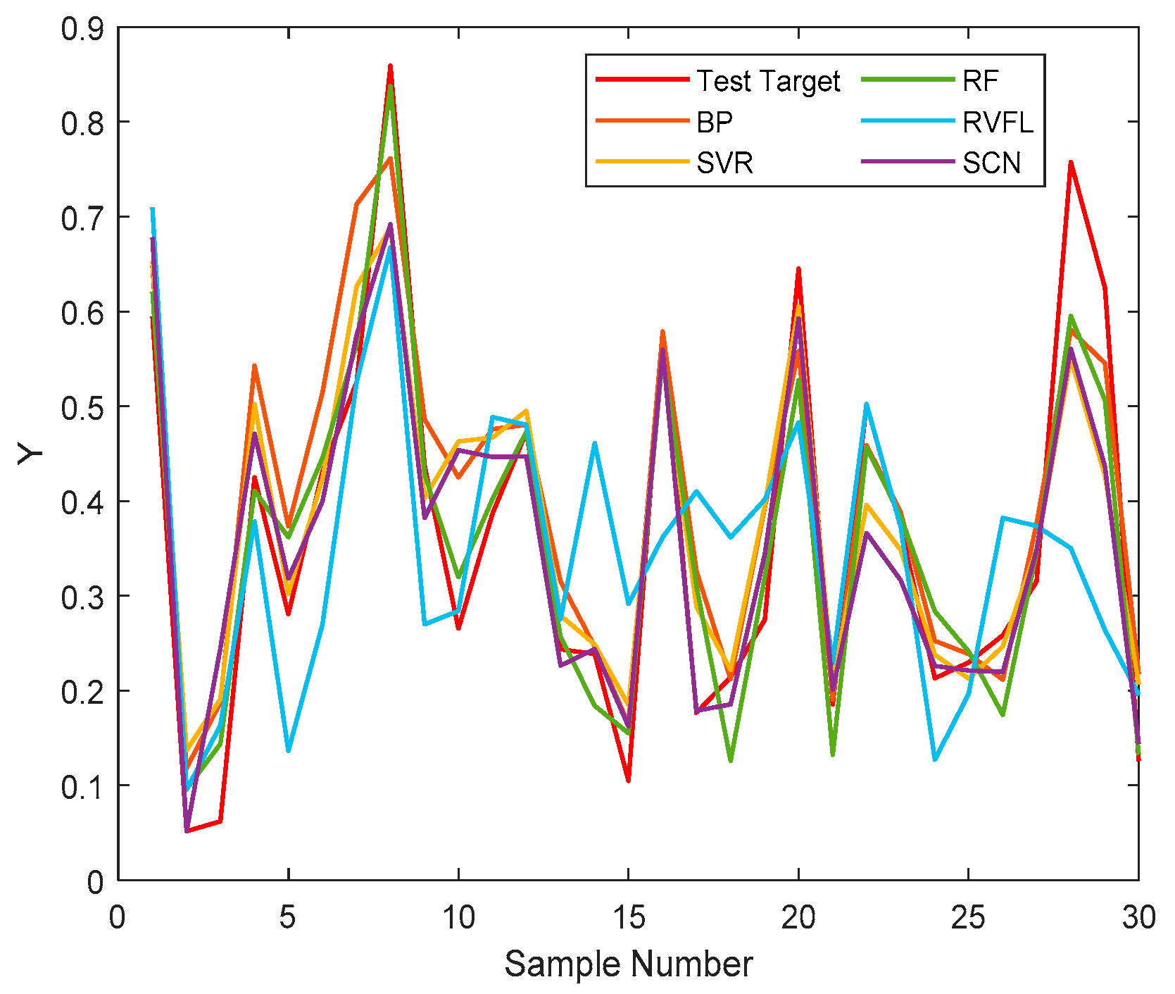
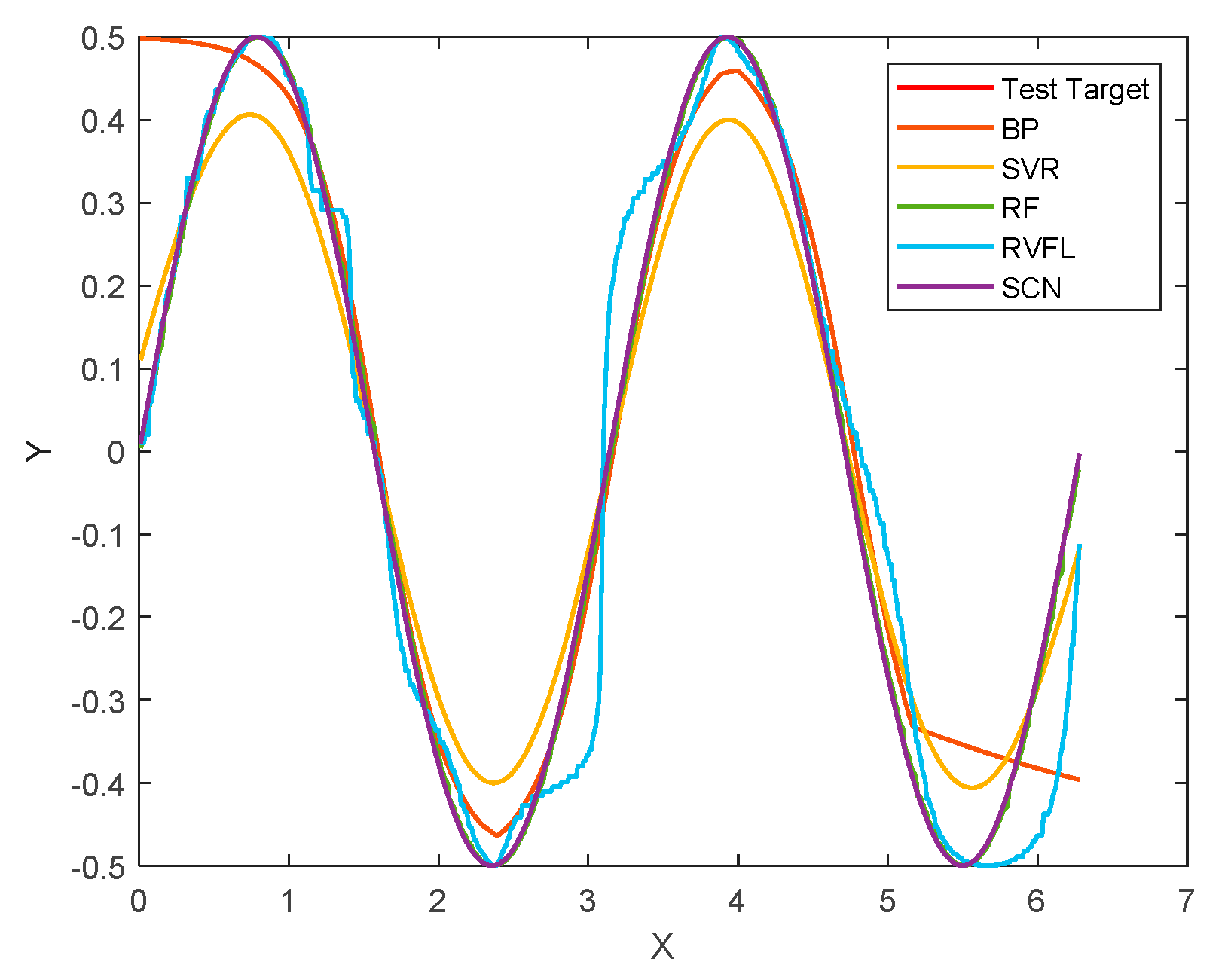
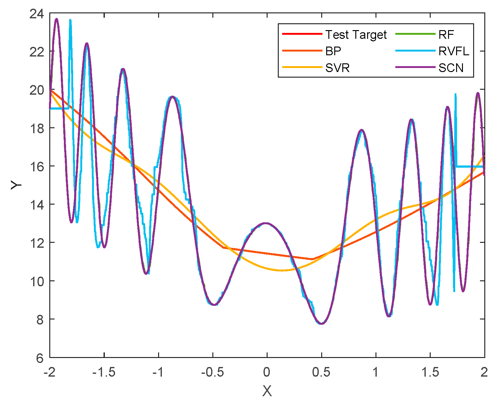
4.2. Performance
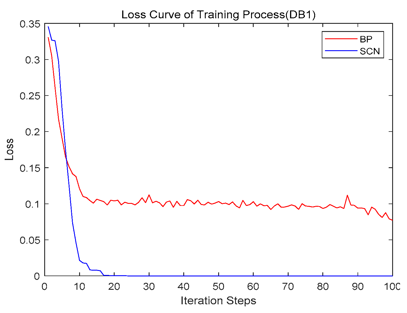
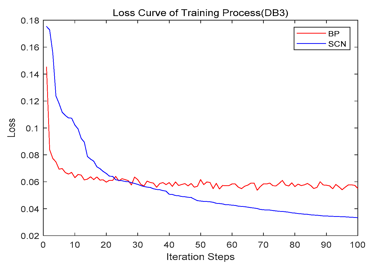
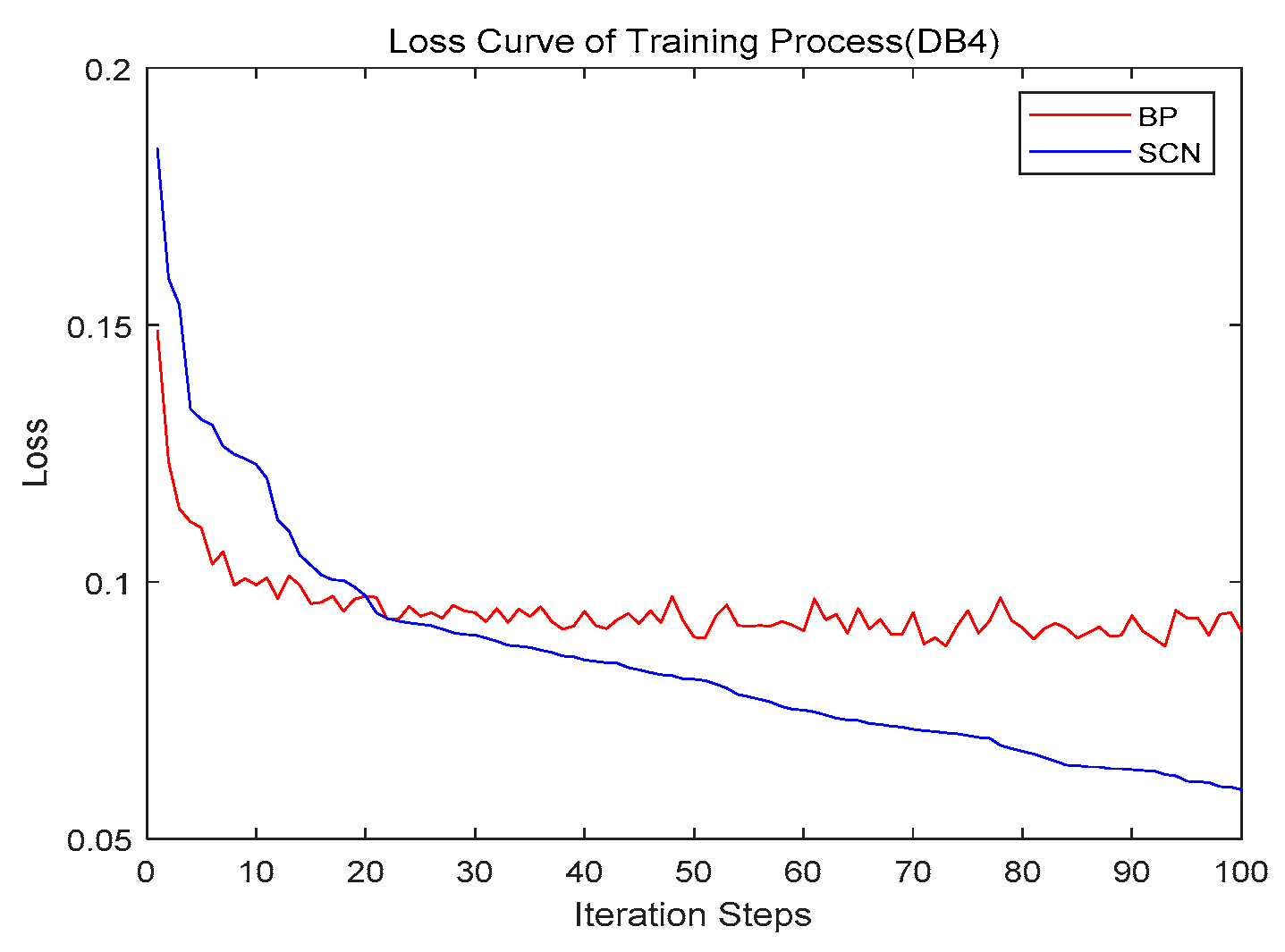
4.3. Convergence
4.4. Stability
4.5. Performance with Various Initial Weights
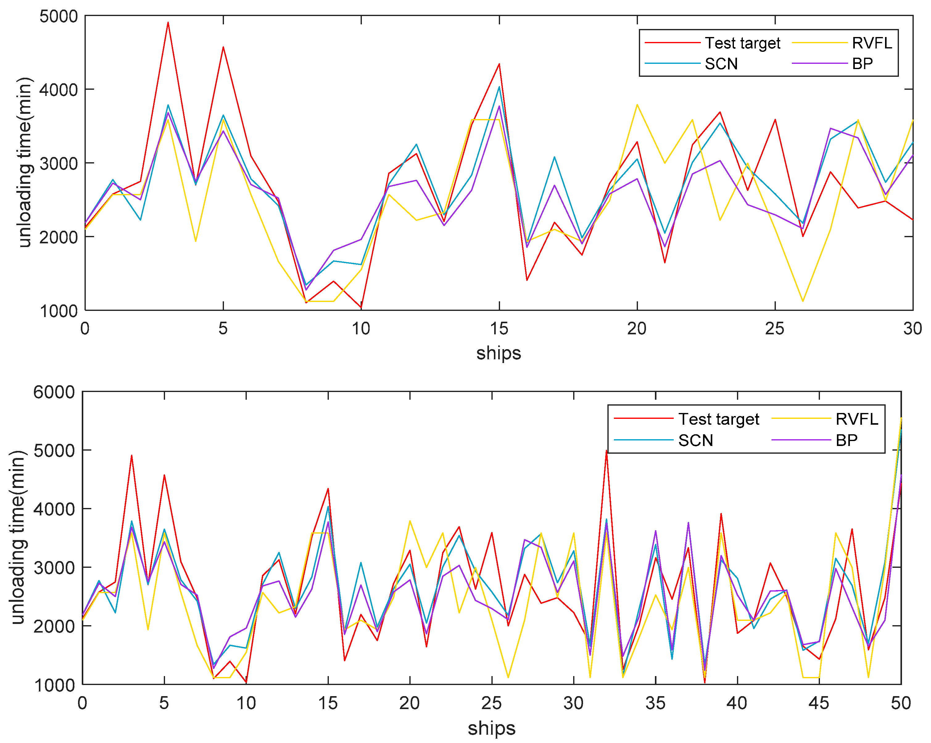
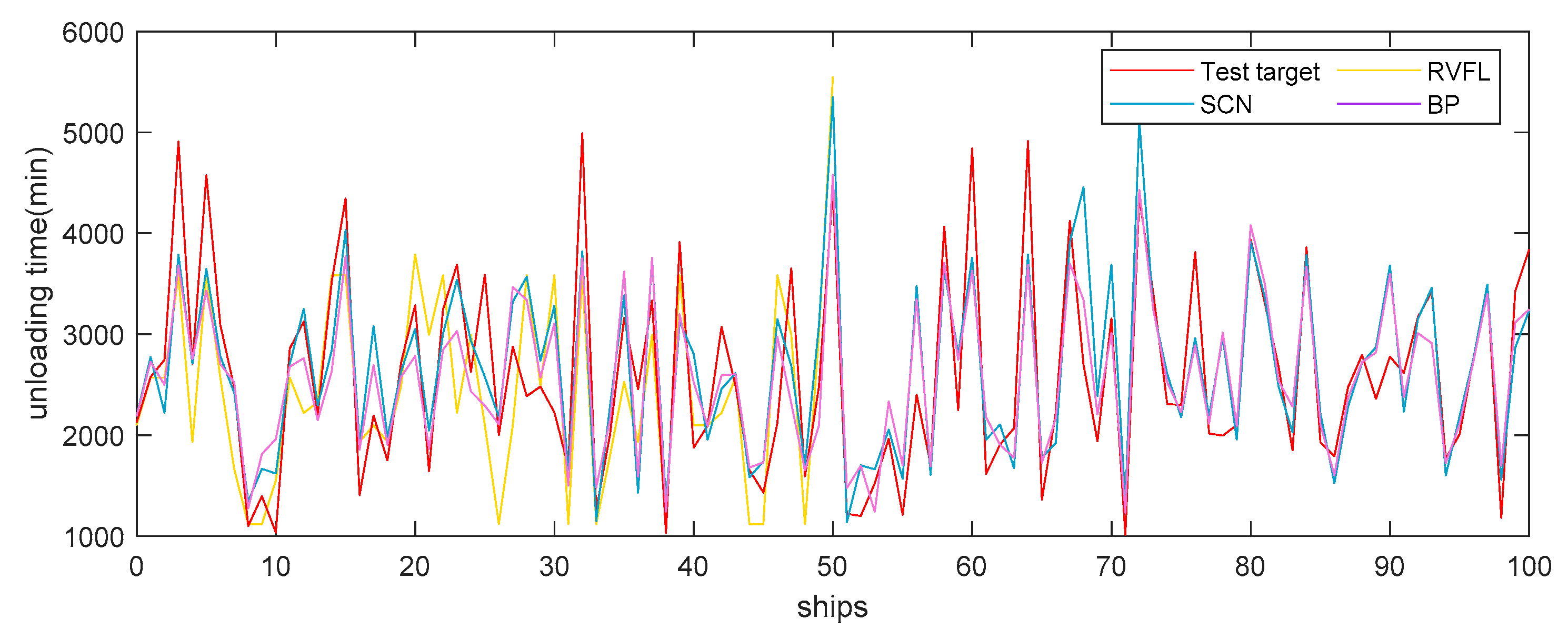
4.6. Case Study
5. Conclusions
Author Contributions
Funding
Institutional Review Board Statement
Informed Consent Statement
Data Availability Statement
Conflicts of Interest
References
- Gao, Z.; Sun, D.; Zhao, R.; Dong, Y. Ship-unloading scheduling optimization for a steel plant. Inf. Sci. 2021, 544, 214–226. [Google Scholar] [CrossRef]
- Gao, Z.; Zhang, M.; Zhang, L. Ship-unloading optimization with differential evolution. Inf. Sci. 2022, 591, 88–102. [Google Scholar] [CrossRef]
- Zhang, X.F.; Chen, S.N.; Zhang, J.X. Adaptive sliding mode consensus control based on neural network for singular fractional order multi-agent systems. Appl. Math. Comput. 2022, 434, 127442. [Google Scholar] [CrossRef]
- Zhang, X.F.; Chen, Y.Q. Admissibility and robust stabilization of continuous linear singular fractional order systems with the fractional order α: The 0 < α < 1 case. ISA Trans. 2018, 82, 42–50. [Google Scholar] [PubMed]
- Yan, H.; Zhang, J.X.; Zhang, X.F. Injected infrared and visible image fusion via L1 decomposition model and guided filtering. IEEE Trans. Comput. Imaging 2022, 8, 162–173. [Google Scholar] [CrossRef]
- Tang, L.; Meng, Y. Data analytics and optimization for smart industry. Front. Eng. Manag. 2021, 8, 157–171. [Google Scholar] [CrossRef]
- Kong, D.; Zhu, J.; Duan, C.; Liu, L.; Chen, D. Bayesian linear regression for surface roughness prediction. Mech. Syst. Signal Process. 2020, 142, 106770. [Google Scholar] [CrossRef]
- An, X.; Jiang, D.; Liu, C.; Zhao, M. Wind farm power prediction based on wavelet decomposition and chaotic time series. Expert Syst. Appl. 2011, 38, 11280–11285. [Google Scholar] [CrossRef]
- Rojas, I.; Valenzuela, O.; Rojas, F.; Guillen, A.; Herrera, L.J.; Pomares, H.; Marquez, L.; Pasadas, M. Soft-computing techniques and ARMA model for time series prediction. Neurocomputing 2008, 71, 519–537. [Google Scholar] [CrossRef]
- Kundrat, D.M. Conceptual model of the iron blast furnace considering thermodynamic and kinetic constraints on the process. Metall. Trans. B 1989, 20, 205–218. [Google Scholar] [CrossRef]
- Gan, L.; Lai, C. A general viscosity model for molten blast furnace slag. Metall. Mater. Trans. B 2014, 45, 875–888. [Google Scholar] [CrossRef]
- Xiao, Z.; Ye, S.J.; Zhong, B.; Sun, C.X. BP neural network with rough set for short term load forecasting. Expert Syst. Appl. 2009, 36, 273–279. [Google Scholar] [CrossRef]
- Adelia, H.; Panakkat, A. A probabilistic neural network for earthquake magnitude prediction. Neural Netw. 2009, 22, 1018–1024. [Google Scholar] [CrossRef] [PubMed]
- Zhang, Y.; Wang, X.; Yu, J.; Zeng, T.; Wang, J. Multistep prediction for earthworks unloading duration: A fuzzy Att-Seq2Seq network with optimal partitioning and multi-time granularity modeling. Neural Comput. Appl. 2023, 35, 21023–21042. [Google Scholar] [CrossRef]
- Liang, S.K.; Wang, C.N. Modularized simulation for lot delivery time forecast in automatic material handling systems of 300 mm semiconductor manufacturing. Int. J. Adv. Manuf. Technol. 2005, 26, 645–652. [Google Scholar] [CrossRef]
- Xu, Y.; Chen, Q.; Quan, X. Robust berth scheduling with uncertain vessel delay and handling time. Ann. Oper. Res. 2012, 192, 123–140. [Google Scholar] [CrossRef]
- Rumelhart, D.E.; Hinton, G.E.; Williams, R.J. Learning representations by back-propagating errors. Nature 1986, 323, 533–536. [Google Scholar] [CrossRef]
- Hornik, K.; Stinchcombe, M.; White, H. Multilayer feedforward networks are universal approximators. Neural Netw. 1989, 2, 359–366. [Google Scholar] [CrossRef]
- Malik, A.K.; Gao, R.; Ganaie, M.A.; Tanveer, M.; Suganthan, P.N. Random vector functional link network: Recent developments, applications, and future directions. Appl. Soft Comput. 2023, 143, 110377. [Google Scholar]
- Wang, D.; Li, M. Stochastic configuration networks: Fundamentals and algorithms. IEEE Trans. Cybern. 2017, 47, 3466–3479. [Google Scholar] [CrossRef]
- Dhingra, V.; Roy, D.; de Koster, R.B.M. A cooperative quay crane-based stochastic model to estimate vessel handling time. Flex. Serv. Manuf. J. 2017, 29, 97–124. [Google Scholar] [CrossRef]
- Bish, E.K. A multiple-crane-constrained scheduling problem in a container terminal. Eur. J. Oper. Res. 2003, 144, 83–107. [Google Scholar] [CrossRef]
- Al-Dhaheri, N.; Jebali, A.; Diabat, A. A simulation-based genetic algorithm approach for the quay crane scheduling under uncertainty. Simul. Model. Pract. Theory 2016, 66, 122–138. [Google Scholar] [CrossRef]
- Sun, D.; Tang, L.; Baldacci, R. A benders decomposition-based framework for solving quay crane scheduling problems. Eur. J. Oper. Res. 2019, 273, 504–515. [Google Scholar] [CrossRef]
- Sammarra, M.; Cordeau, J.F.; Laporte, G.; Monaco, M.F. A tabu search heuristic for the quay crane scheduling problem. J. Sched. 2007, 10, 327–336. [Google Scholar] [CrossRef]
- Tang, L.; Zhao, J.; Liu, J. Modeling and solution of the joint quay crane and truck scheduling problem. Eur. J. Oper. Res. 2014, 236, 978–990. [Google Scholar] [CrossRef]
- Kao, C.; Li, D.C.; Wu, C.; Tsai, C.C. Knowledge-based approach to the optimal dock arrangement. Int. J. Syst. Sci. 1990, 21, 2209–2215. [Google Scholar] [CrossRef]
- Kao, C.; Wu, C.; Li, D.C.; Lai, C.Y. Scheduling ship discharging via knowledge transformed heuristic evaluation function. Int. J. Syst. Sci. 1992, 23, 631–639. [Google Scholar] [CrossRef]
- Kao, C.; Lee, H.T. Coordinated dock operations: Integrating dock arrangement with ship discharging. Comput. Ind. 1996, 28, 113–122. [Google Scholar] [CrossRef]
- Kim, K.H.; Moon, K.C. Berth scheduling by simulated annealing. Transp. Res. Part B 2003, 37, 541–560. [Google Scholar] [CrossRef]
- Kim, B.I.; Chang, S.Y.; Chang, J.; Han, Y.; Koo, J.; Lim, K.; Shin, J.; Jeong, S.; Kwak, W. Scheduling of raw-material unloading from ships at a steelworks. Prod. Plan. Control 2011, 22, 389–402. [Google Scholar] [CrossRef]
- Lee, D.H.; Cao, J.X.; Shi, Q.; Chen, J.H. A heuristic algorithm for yard truck scheduling and storage allocation problems. Transp. Res. Part E 2009, 45, 810–820. [Google Scholar] [CrossRef]
- Tang, X.; Jin, J.G.; Shi, X. Stockyard storage space allocation in large iron ore terminals. Comput. Ind. Eng. 2002, 164, 107911. [Google Scholar] [CrossRef]
- Li, S.; Tang, L. Improved tabu search algorithms for storage space allocation in integrated iron and steel plant. In Proceedings of the 2005 ICSC Congress on Computational Intelligence Methods and Applications, Istanbul, Turkey, 15–17 December 2005; p. 6. [Google Scholar] [CrossRef]
- Kim, B.I.; Koo, J.; Park, B.S. A raw material storage yard allocation problem for a large-scale steelwork. Int. J. Adv. Manuf. Technol. 2009, 41, 880–884. [Google Scholar] [CrossRef]
- Zhang, B.; Shin, Y.C. A probabilistic neural network for uncertainty prediction with applications to manufacturing process monitoring. Appl. Soft Comput. 2022, 124, 108995. [Google Scholar] [CrossRef]
- Li, W.; Wang, X.X.; Han, H.G.; Qiao, J. A PLS-based pruning algorithm for simplified long-short term memory neural network in time series prediction. Knowl.-Based Syst. 2022, 254, 109608. [Google Scholar] [CrossRef]
- Kosanoglu, F. Wind speed forecasting with a clustering-based deep learning model. Appl. Sci. 2022, 12, 13031. [Google Scholar] [CrossRef]
- Hussein, A.M.; Elaziz, M.A.; Abdel Wahed, M.S.M.; Sillanpää, M. A new approach to predict the missing values of algae during water quality monitoring programs based on a hybrid moth search algorithm and the random vector functional link network. J. Hydrol. 2019, 575, 852–863. [Google Scholar] [CrossRef]
- El-Said, E.M.S.; Elaziz, M.A.; Elsheikh, A.H. Machine learning algorithms for improving the prediction of air injection effect on the thermohydraulic performance of shell and tube heat exchanger. Appl. Therm. Eng. 2021, 185, 116471. [Google Scholar] [CrossRef]
- Wang, W.; Wang, D. Prediction of component concentrations in sodium aluminate liquor using stochastic configuration networks. Neural Comput. Appl. 2020, 32, 13625–13638. [Google Scholar] [CrossRef]
- Li, K.; Yang, C.; Wang, W.; Qiao, J. An improved stochastic configuration network for concentration prediction in wastewater treatment process. Inf. Sci. 2023, 622, 148–160. [Google Scholar] [CrossRef]


| Dataset | Number 1 | Number 2 | Range |
|---|---|---|---|
| DB1 | 5 | 30 | [0, 50] |
| DB2 | 10 | 40 | [0, 50] |
| DB3 | 50 | 10 | [0, 50] |
| DB4 | 30 | 5 | [0, 50] |
| Dataset | Number | Range-1 | Range-2 |
|---|---|---|---|
| DB1 | 80 | [−40, 40] | [−50, 50] |
| DB2 | 100 | [−20, 20] | [−50, 50] |
| DB3 | 100 | [−5, 5] | [−50, 50] |
| DB4 | 100 | [−10, 10] | [−50, 50] |
| Dataset | Model | RMSE | MAPE | R2 | ||
|---|---|---|---|---|---|---|
| Mean ± (SD) | Best | Mean ± (SD) | Best | |||
| DB1 | SVR | 0.0703 ± 0.0002 | 0.0700 | 30.1491 ± 0.9152 | 28.3137 | 0.0045 |
| RF | 0.0085 ± 0.0007 | 0.0076 | 7.7704 ± 2.7491 | 3.7731 | 0.9994 | |
| BP | 0.0122 ± 0.0123 | 0.0115 | 37.6948 ± 23.3176 | 13.7574 | 0.9976 | |
| RVFL | 0.0484 ± 0.0006 | 0.0484 | 66.1857 ± 14.4562 | 39.9376 | 0.9824 | |
| SCN | 0.0074 ± 0.0024 | 0.0024 | 5.6983 ± 2.6124 | 0.8440 | 0.9995 | |
| DB2 | SVR | 0.1996 ± 0.0009 | 0.1982 | 21.4102 ± 0.1986 | 21.1481 | 0.0594 |
| RF | 0.0064 ± 0.0005 | 0.0056 | 0.4135 ± 0.0150 | 0.3944 | 0.9993 | |
| BP | 0.0761 ± 0.0100 | 0.0601 | 6.2884 ± 1.9444 | 6.4121 | 0.9063 | |
| RVFL | 0.1084 ± 0.0005 | 0.1084 | 7.3193 ± 0.0225 | 7.3171 | 0.8197 | |
| SCN | 0.0008 ± 0.0039 | 0.0008 | 0.0050 ± 0.0008 | 0.0038 | 0.9999 | |
| DB3 | SVR | 0.0536 ± 0.0027 | 0.0492 | 2.7469 ± 0.1562 | 2.5131 | 0.9460 |
| RF | 0.03968 ± 0.0036 | 0.0333 | 1.9413 ± 0.1555 | 1.6562 | 0.9649 | |
| BP | 0.0602 ± 0.0155 | 0.0386 | 10.4826 ± 1.9601 | 7.5725 | 0.9454 | |
| RVFL | 0.0687 ± 0.0001 | 0.0686 | 14.2589 ± 0.0001 | 14.2578 | 0.9170 | |
| SCN | 0.0388 ± 0.0012 | 0.0357 | 1.8707 ± 0.0483 | 1.7650 | 0.9681 | |
| DB4 | SVR | 0.0885 ± 0.0045 | 0.0823 | 20.8771 ± 1.0710 | 19.1571 | 0.8147 |
| RF | 0.0961 ± 0.0080 | 0.0785 | 18.3751 ± 1.1851 | 16.4298 | 0.7839 | |
| BP | 0.0911 ± 0.0087 | 0.0796 | 19.5973 ± 1.7310 | 17.1850 | 0.8029 | |
| RVFL | 0.1932 ± 0.0001 | 0.1922 | 41.6601 ± 2.4803 | 33.1910 | 0.4144 | |
| SCN | 0.0870 ± 0.0060 | 0.0767 | 21.8238 ± 1.2261 | 19.3793 | 0.8135 | |
| Range of Weights | DB1 | ||
|---|---|---|---|
| RVFL | BP | SCN | |
| [−1, 1] | 0.28148 | 0.14596 | 0.00586 |
| [−5, 5] | 0.13976 | 0.49169 | 0.00678 |
| [−10, 10] | 0.08151 | 0.56205 | 0.00748 |
| [−20, 20] | 0.05453 | 0.59831 | 0.00877 |
| [−30, 30] | 0.04694 | 0.61142 | 0.00837 |
| [−40, 40] | 0.04878 | 0.61564 | 0.00895 |
| [−50, 50] | 0.05661 | 0.56205 | 0.00897 |
| [−60, 60] | 0.16208 | 0.56205 | 0.00968 |
| [−80, 80] | 0.21759 | 0.60772 | 0.00995 |
| [−100, 100] | 0.16081 | 0.61610 | 0.00954 |
| [−500, 500] | 0.25634 | 0.61374 | 0.01169 |
| Range of Weights | DB2 | ||
|---|---|---|---|
| RVFL | BP | SCN | |
| [−1, 1] | 0.18356 | 0.20413 | 0.00474 |
| [−5, 5] | 0.12167 | 0.52918 | 0.00704 |
| [−10, 10] | 0.09808 | 0.54208 | 0.00817 |
| [−20, 20] | 0.09679 | 0.53724 | 0.00582 |
| [−30, 30] | 0.08942 | 0.57866 | 0.00853 |
| [−40, 40] | 0.09056 | 0.60472 | 0.00962 |
| [−50, 50] | 0.10127 | 0.56014 | 0.00937 |
| [−60, 60] | 0.14049 | 0.59212 | 0.00942 |
| [−80, 80] | 0.16943 | 0.56078 | 0.00966 |
| [−100, 100] | 0.16799 | 0.51073 | 0.01021 |
| [−500, 500] | 0.31912 | 0.54241 | 0.01235 |
| Range of Weights | DB3 | ||
|---|---|---|---|
| RVFL | BP | SCN | |
| [−1, 1] | 0.07325 | 0.04593 | 0.03709 |
| [−5, 5] | 0.04759 | 0.50602 | 0.07701 |
| [−10, 10] | 0.04287 | 0.57113 | 0.07612 |
| [−20, 20] | 0.07698 | 0.04606 | 0.07848 |
| [−30, 30] | 0.09410 | 0.55866 | 0.10125 |
| [−40, 40] | 0.10406 | 0.52318 | 0.09185 |
| [−50, 50] | 0.12092 | 0.53317 | 0.08473 |
| [−60, 60] | 0.12194 | 0.53291 | 0.08901 |
| [−80, 80] | 0.13108 | 0.53027 | 0.08757 |
| [−100, 100] | 0.12379 | 0.54040 | 0.08571 |
| [−500, 500] | 0.13252 | 0.55592 | 0.08917 |
| Range of Weights | DB4 | ||
|---|---|---|---|
| RVFL | BP | SCN | |
| [−1, 1] | 0.18387 | 0.09637 | 0.10241 |
| [−5, 5] | 0.13977 | 0.40924 | 0.10093 |
| [−10, 10] | 0.14436 | 0.57055 | 0.09312 |
| [−20, 20] | 0.17075 | 0.55035 | 0.10734 |
| [−30, 30] | 0.19714 | 0.56227 | 0.13241 |
| [−40, 40] | 0.20660 | 0.53162 | 0.12498 |
| [−50, 50] | 0.21126 | 0.55677 | 0.10198 |
| [−60, 60] | 0.21676 | 0.55245 | 0.10081 |
| [−80, 80] | 0.22001 | 0.56567 | 0.10748 |
| [−100, 100] | 0.23056 | 0.55152 | 0.09669 |
| [−500, 500] | 0.24482 | 0.50343 | 0.10091 |
| Algorithm | DB1 | DB2 | DB3 | DB4 | ||||
|---|---|---|---|---|---|---|---|---|
| Mean | Std | Mean | Std | Mean | Std | Mean | Std | |
| RVFL | 0.13695 | 0.08663 | 0.14349 | 0.06779 | 0.09719 | 0.03276 | 0.19690 | 0.03396 |
| BP | 0.54425 | 0.13744 | 0.52384 | 0.10962 | 0.44942 | 0.20026 | 0.49548 | 0.14010 |
| SCN | 0.00873 | 0.00160 | 0.00863 | 0.00213 | 0.08164 | 0.01646 | 0.10628 | 0.01192 |
| BN | SN | RMN | QRM | UD | ST | ET | SL1 | SL2 |
|---|---|---|---|---|---|---|---|---|
| 7 | FS8 | Ore fines 1 | 23,585 | 37 | 5 November 2018 15:00 | 7 November 2018 4:00 | 173 | OB24 |
| 1 | MT | OYD-S/ONM-N | 51,500 | 23 | 5 November 2018 9:00 | 6 November 2018 8:00 | 292 | OA16 |
| 1 | BY | OHY-S | 90,000 | 34 | 7 November 2018 10:00 | 8 November 2018 20:00 | 320 | OA18 |
| 2 | ZC258 | Ore fines 4 | 33,000 | 35 | 5 November 2018 9:00 | 6 November 2018 20:00 | 189 | OB32 |
| 4 | BXH6 | dolomite | 1100 | 3 | 5 November 2018 13:00 | 5 November 2018 16:00 | 50 | OC23 |
| 5 | JN9 | Limestone | 5005 | 18 | 6 November 2018 2:00 | 6 November 2018 20:00 | 110 | OC11 |
| 2 | ZC258 | Ore fines 4 | 12,000 | 13 | 6 November 2018 9: 00 | 6 November 2018 22:00 | 189 | OB16 |
| 2 | BY | OHY-S | 90,000 | 34 | 7 November 2018 3:30 | 8 November 2018 20:00 | 320 | OA36 |
| 4 | JN9 | Limestone | 5005 | 17 | 6 November 2018 9:00 | 7 November 2018 2:00 | 110 | OC26 |
Disclaimer/Publisher’s Note: The statements, opinions and data contained in all publications are solely those of the individual author(s) and contributor(s) and not of MDPI and/or the editor(s). MDPI and/or the editor(s) disclaim responsibility for any injury to people or property resulting from any ideas, methods, instructions or products referred to in the content. |
© 2024 by the authors. Licensee MDPI, Basel, Switzerland. This article is an open access article distributed under the terms and conditions of the Creative Commons Attribution (CC BY) license (https://creativecommons.org/licenses/by/4.0/).
Share and Cite
Gao, Z.; Li, D.; Wang, D.; Yu, Z.; Pedrycz, W.; Wang, X. Prediction of Ship-Unloading Time Using Neural Networks. Appl. Sci. 2024, 14, 8213. https://doi.org/10.3390/app14188213
Gao Z, Li D, Wang D, Yu Z, Pedrycz W, Wang X. Prediction of Ship-Unloading Time Using Neural Networks. Applied Sciences. 2024; 14(18):8213. https://doi.org/10.3390/app14188213
Chicago/Turabian StyleGao, Zhen, Danning Li, Danni Wang, Zengcai Yu, Witold Pedrycz, and Xinhai Wang. 2024. "Prediction of Ship-Unloading Time Using Neural Networks" Applied Sciences 14, no. 18: 8213. https://doi.org/10.3390/app14188213
APA StyleGao, Z., Li, D., Wang, D., Yu, Z., Pedrycz, W., & Wang, X. (2024). Prediction of Ship-Unloading Time Using Neural Networks. Applied Sciences, 14(18), 8213. https://doi.org/10.3390/app14188213