Numerical Modeling of Scholte Wave in Acoustic-Elastic Coupled TTI Anisotropic Media

Abstract

Numerical modeling of acoustic-elastic media is helpful for seismic exploration in the deepwater environment. We propose an algorithm based on the staggered grid finite difference to simulate wave propagation in the interface between fluid and transversely isotropic media, where the interface does not need to consider the boundary condition. We also derive the stability conditions of the proposed method. Scholte waves, which are generated at the seafloor, exhibit distinctly different propagation behaviors than body waves in ocean-bottom seismograms. Numerical examples are used to characterize the wavefield of Scholte waves and discuss the relationship between travel time and the Thomsen parameters. Thomsen parameters are assigned clear physical meanings, and the magnitude of their values directly indicates the strength of the anisotropy in the media. Numerical results show that the velocity of the Scholte wave is positively correlated with ε and negatively correlated with δ. And the curve of the arrival time of the Scholte wave as a whole is sinusoidal and has no symmetry in inclination. The velocity of the Scholte wave in azimuth is positively related to the polar angle. The energy of the Scholte wave is negatively correlated with the distance from the source to the fluid-solid interface. The above results provide a basis for studying oceanic Scholte waves and are beneficial for utilizing the information provided by Scholte waves.

1. Introduction

Numerical modeling of acoustic-elastic coupled media is critical to the interpretation of shallow sea seismic data, and the accurate numerical simulation is of great significance for the later data processing and parameters inversion [1,2]. However, the accurate simulation of the fluid-solid interface and construction of the Scholte waves are very challenging and are the signature problems in this research [3,4,5,6,7]. An additional challenge is the introduction of anisotropy in the research, and the assumption of isotropy can lead to the wrong imaging of underground structures and the reduction of resolution [8,9,10,11].

Scholte waves are generated at a fluid-solid interface. Their energy is mainly distributed in the fluid, while the energy decays with depth in the solid [12,13,14,15,16,17]. Similarly, there are also leaked Rayleigh waves at a fluid-solid interface, whose energy decays with depth in the solid with propagation characteristics similar to head waves [18]. Numerical studies have summarized the physical aspects of Scholte waves [19,20,21,22]. If the value of the fluid sound velocity $C_f$ is between the solid shear wave velocity $C_s$ and the longitudinal wave velocity $C_L$, Scholte waves can be generated at a fluid-solid interface. If $C_f<C_s$, leaked Rayleigh waves are generated. If the acoustic impedance mismatch is large, the Scholte wave velocity is close to $C_f$. Scholte waves do not decay along the direction of propagation, but lose energy in 3D due to geometric effect.

There are two wavefield simulation approaches for modeling wave propagation in acoustic-elastic coupled media: (1) the partitioned approach [23,24,25,26], where the acoustic wave equation and the elastic wave equation are used to describe wave propagation in fluid and solid phases, respectively. The partitioned method needs accurate kinematic and dynamic boundary conditions. A fluid-solid interface is usually treated with special mesh and coordinate mapping to match the two boundary conditions [27,28,29]; (2) the monolithic approach [30,31,32,33,34], where the elastic velocity-stress equation governs the wavefield in two-phase media without providing specific boundary conditions. Based on the wave equation, the synthetic pressure field is substituted into the first-order elastic velocity-stress equation; the first-order acoustic-elastic coupled equation is derived [33,34]. The equation has accurate kinematic and dynamic characteristics, successfully simulates Scholte waves, and solves the artifact problem at the fluid-solid interface [31]. With the development of the research, vertical transverse isotropy (VTI) was introduced into the acoustic-elastic coupled equation [35].

It is now accepted that anisotropy media exists widely. Increasingly practical work has introduced anisotropy [36,37], which greatly improved the imaging quality of underground structures and the interpretability of data [38,39]. Anisotropy is also essential for the research of acoustic-elastic coupled media. Researchers demonstrated the presence of anisotropy in the salt floor of the Gulf of Mexico from seismic imaging using ocean-bottom data and borehole data [40]. Combined with the mimetic finite difference method (MFD) and fully staggered mesh (FSGs), the wavefield of VTI acoustic-elastic coupled media is accurately simulated [29]. Here, we define the underwater solid media as TTI (Tilted Transverse Isotropy) media, which is a type of transversely isotropic (TI) media with a tilted axis of symmetry. TTI media have different velocities along the axis of symmetry and perpendicular to the axis of symmetry. It can be seen as a tilted form of VTI (Vertical Transverse Isotropy) media with a vertical axis of symmetry. And we describe Scholte waves in 3D integrally to understand characteristics of the Scholte wave.

In this paper, we adopt the monolithic approach to simulate the wavefield of acoustic-elastic coupled TTI media. We start from the 2D first-order VTI acoustic-elastic coupled equation [35] and extend it through the Bond matrix transformation [41]. The main purpose of this paper is to construct the 3D first-order TTI acoustic-elastic coupled equation and discusses the characteristics of Scholte waves in snapshots [42]. First, we introduce some essential preliminaries. Then, we give the 3D first-order TTI acoustic-elastic coupled equation and introduce the Bond transformation in the derivation process. Then, we show the staggered-grid finite difference (FD) form of the new equation and the exact stability conditions [24,43,44], which can preserve the dispersion relation in a reasonable frequency range [45,46]. Numerical examples are used to analyze the simulated wavefields of 2D models, 3D models, and a random model, and to describe Scholte waves completely. Finally, we give our conclusions and provide a technical appendix with mathematical details.

2. Wave Equations

2.1. Acoustic-Elastic Coupled Equation

Following the form of Yu [35], we derive the 3D TTI acoustic-elastic coupled equation (see Appendix A):

$$\begin{array}{c}\rho {\displaystyle \frac{\partial }{\partial \mathrm{t}}}\mathrm{V}=\mathrm{L}\varphi ,\\ {\displaystyle \frac{\partial }{\partial \mathrm{t}}}\varphi ={\mathrm{D}}^{ae}{\mathrm{L}}^{\mathrm{T}}\mathrm{V}+\mathrm{f},\end{array}$$

(1)

where $\rho$ is density, $t$ is time, $\mathrm{V}={\left({\mathrm{v}}_{\mathrm{x}},{\mathrm{v}}_{\mathrm{y}},{\mathrm{v}}_{\mathrm{z}}\right)}^{\mathrm{T}}$ is velocity vector of particle, $\varphi ={\left({\mathrm{P}}_{\mathrm{s}},{\tau }_{\mathrm{xx}}^{\mathrm{s}},{\tau }_{\mathrm{yy}}^{\mathrm{s}},{\tau }_{\mathrm{zz}}^{\mathrm{s}},{\tau }_{\mathrm{xy}}^{\mathrm{s}},{\tau }_{\mathrm{xz}}^{\mathrm{s}},{\tau }_{\mathrm{yz}}^{\mathrm{s}}\right)}^{\mathrm{T}}$ is a vector composed of synthetic pressure field and deviator stress, $\mathrm{f}$ represents source, $\mathrm{L}$ represents partial differential operator, ${\mathrm{D}}^{ae}$ is the stiffness coefficient matrix for TTI acoustic-elastic coupled equation, and ${\mathrm{D}}_{ij}$ is the stiffness coefficient of TTI media.

$$\mathrm{L}=\left[\begin{array}{ccccccc}-{\displaystyle \frac{\partial }{\partial x}}& {\displaystyle \frac{\partial }{\partial x}}& 0& 0& {\displaystyle \frac{\partial }{\partial y}}& {\displaystyle \frac{\partial }{\partial z}}& 0\\ -{\displaystyle \frac{\partial }{\partial y}}& 0& {\displaystyle \frac{\partial }{\partial y}}& 0& {\displaystyle \frac{\partial }{\partial x}}& 0& {\displaystyle \frac{\partial }{\partial z}}\\ -{\displaystyle \frac{\partial }{\partial z}}& 0& 0& {\displaystyle \frac{\partial }{\partial z}}& 0& {\displaystyle \frac{\partial }{\partial x}}& {\displaystyle \frac{\partial }{\partial y}}\end{array}\right],$$

(2)

and

$${\mathrm{D}}^{\mathit{ae}}=\left[\begin{array}{ccccccc}0& -\frac{D_{11}+D_{12}+D_{13}}{3}& -\frac{D_{12}+D_{22}+D_{23}}{3}& -\frac{D_{13}+D_{23}+D_{33}}{3}& 0& -\frac{D_{15}+D_{25}+D_{35}}{3}& 0\\ 0& \frac{2D_{11}+D_{12}+D_{13}}{3}& \frac{2D_{12}+D_{22}+D_{23}}{3}& \frac{2D_{13}+D_{23}+D_{33}}{3}& 0& \frac{2D_{15}+D_{25}+D_{35}}{3}& 0\\ \mathrm{}& \frac{2D_{12}+D_{11}+D_{13}}{3}& \frac{2D_{22}+D_{12}+D_{23}}{3}& \frac{2D_{23}+D_{13}+D_{33}}{3}& 0& \frac{2D_{25}+D_{15}+D_{35}}{3}& 0\\ 0& \frac{2D_{13}+D_{12}+D_{11}}{3}& \frac{2D_{23}+D_{22}+D_{13}}{3}& \frac{2D_{33}+D_{23}+D_{13}}{3}& 0& \frac{2D_{35}+D_{25}+D_{15}}{3}& 0\\ 0& 0& 0& 0& D_{44}& 0& D_{46}\\ 0& D_{15}& D_{25}& D_{35}& 0& D_{55}& 0\\ 0& 0& 0& 0& D_{46}& 0& D_{66}\end{array}\right].$$

(3)

2.2. Bond Transformation

Introducing the matrix of elastic coefficients of the TTI media is the key to deriving the 3D TTI acoustic-elastic coupled equation. Thus, we perform coordinate rotation on VTI media to obtain the elastic coefficient matrix of TTI media.

As shown in Figure 1, $\theta$ is the polar angle and $\phi$ is the azimuth angle. The elastic coefficient matrix of TTI media can be obtained by rotating VTI twice.

We consider both the polar angle and the azimuth angle:

$$\mathrm{D}={\mathrm{TRCR}}^{\mathrm{T}}{\mathrm{T}}^{\mathrm{T}},$$

(4)

where $\mathrm{D}$ is the elastic coefficient matrix of TTI media, and $\mathrm{R}$ and $\mathrm{T}$ are the newly defined conversion matrices.

$$\mathrm{R}=\left(\begin{array}{cccccc}{\cos }^2\theta & 0& {\sin }^2\theta & 0& -\sin 2\theta & 0\\ 0& 1& 0& 0& 0& 0\\ {\sin }^2\theta & 0& {\cos }^2\theta & 0& \sin 2\theta & 0\\ 0& 0& 0& \cos \theta & 0& \sin \theta \\ {\displaystyle \frac{1}{2}}\sin 2\theta & 0& -{\displaystyle \frac{1}{2}}\sin 2\theta & 0& \cos 2\theta & 0\\ 0& 0& 0& -\sin \theta & 0& \cos \theta \end{array}\right),$$

(5)

$$\mathrm{T}=\left(\begin{array}{cccccc}{\cos }^2\phi & {\sin }^2\phi & 0& 0& 0& -\sin 2\phi \\ {\sin }^2\phi & {\cos }^2\phi & 0& 0& 0& \sin 2\phi \\ 0& 0& 1& 0& 0& 0\\ 0& 0& 0& \cos \phi & \sin \phi & 0\\ 0& 0& 0& -\sin \phi & \cos \phi & 0\\ {\displaystyle \frac{1}{2}}\sin 2\phi & -{\displaystyle \frac{1}{2}}\sin 2\phi & 0& 0& 0& \cos 2\phi \end{array}\right)$$

(6)

3. Staggered-Grid Finite Difference

In the forward seismic simulation, the staggered grid finite difference method is commonly used to solve the wave equation in the time and space domain. It facilitates the incorporation of boundary conditions of the perfectly matched layer, and the derivative weight decays quickly near the derivative point. The even-order difference accuracy increases with the increase of the approximate order.

According to the staggered form of the 3D acoustic-elastic coupled equation in the time and space domain, we define the different components of each physical quantity on the grid points of the staggered grid (Figure 2).

However, their definitions are not arbitrary, and the accuracy of calculations and the smoothness of data cannot be guaranteed. The stability condition can precisely solve this problem. It can guide how to set the temporal step and spatial step to ensure the stability of numerical methods. Below, we will provide a brief introduction, which can be found in Appendix B.

Stability Condition

Equation (1) can be expressed as,

$${\displaystyle \frac{\partial \mathrm{u}}{\partial t}}=\mathrm{Au},$$

(7)

where $\mathrm{u}={\left({\mathrm{v}}_{\mathrm{x}},{\mathrm{v}}_{\mathrm{y}},{\mathrm{v}}_{\mathrm{z}},{\mathrm{P}}_{\mathrm{s}},{\tau }_{\mathrm{xx}}^{\mathrm{s}},{\tau }_{\mathrm{yy}}^{\mathrm{s}},{\tau }_{\mathrm{zz}}^{\mathrm{s}},{\tau }_{\mathrm{xy}}^{\mathrm{s}},{\tau }_{\mathrm{xz}}^{\mathrm{s}},{\tau }_{\mathrm{yz}}^{\mathrm{s}}\right)}^{\mathrm{T}}$. $\mathrm{A}$ is determined by the matrix $\mathrm{L}$ and ${\mathrm{D}}^{ae}$ (the expression for A is given by Equation (A21) of Appendix B). Based on the matrix eigenvalue analysis method [24,43,44], we derive the stability condition for our acoustic-solid coupled wave equations for TTI media (the details are shown in Appendix B):

$$0\le {\displaystyle \frac{\Delta t^2}{\rho }}\left(D_{11}\Delta x^2+D_{44}\Delta y^2+D_{55}\Delta z^2+2D_{15}\Delta x\Delta z\right){\left[{\displaystyle \sum }_{n=1}^N\left|a_n\right|\right]}^2\le 1,$$

(8)

$$0\le {\displaystyle \frac{\Delta t^2}{\rho }}\left(D_{44}\Delta x^2+D_{22}\Delta y^2+D_{66}\Delta z^2+2D_{46}\Delta x\Delta z\right){\left[{\displaystyle \sum }_{n=1}^N\left|a_n\right|\right]}^2\le 1,$$

(9)

$$0\le {\displaystyle \frac{\Delta t^2}{\rho }}\left(D_{55}\Delta x^2+D_{66}\Delta y^2+D_{33}\Delta z^2+2D_{35}\Delta x\Delta z\right){\left[{\displaystyle \sum }_{n=1}^N\left|a_n\right|\right]}^2\le 1,$$

(10)

where $a_n$ are difference coefficients and ${\mathrm{D}}_{ij}$ is the stiffness coefficient of TTI media.

Setting $\Delta x=\Delta y=\Delta z=h$, the stability condition is simplified as

$$\sqrt{5}{\displaystyle \frac{\Delta \mathrm{t}}{\mathrm{h}}}\sqrt{{\displaystyle \frac{\mathrm{S}}{\rho }}}\le {\displaystyle \frac{1}{{{\displaystyle \sum }}_{\mathrm{n}=1}^{\mathrm{N}}\left|{\mathrm{a}}_{\mathrm{n}}\right|}},$$

(11)

where $S=\max \left\{D_{11},D_{22},D_{33},D_{44},D_{55},D_{66},D_{15},D_{35},D_{46}\right\}$. Therefore, we can determine the appropriate temporal and spatial step to ensure a stable calculation process and high-precision data with the physical parameters of the model.

4. Numerical Experiments

In this section, numerical examples are used to illustrate Scholte wave propagation in acoustic-elastic coupled media. We chose to verify the algorithm by comparing it with the spectral element method (SEM) [47] in 2D condition. Afterwards, we will apply the algorithm to 3D and inhomogeneous models.

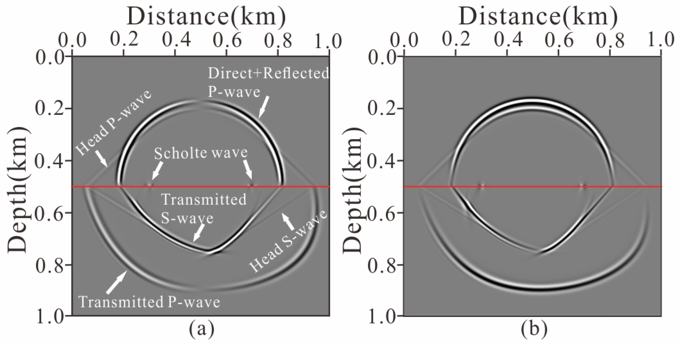
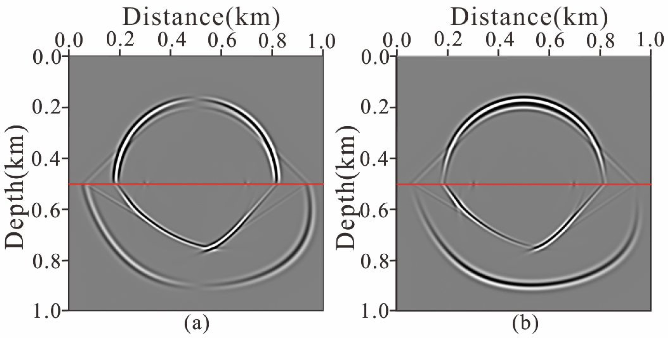
4.1. 2D Two-Layer Acoustic-Elastic Coupled Model

First, we design a two-layer acoustic-elastic coupled model, where the upper and lower layer are fluid and TTI solid (Figure 3). The size of the model is $2 \mathrm{km}\times 2 \mathrm{km}$. The grid spacing is $\Delta x=\Delta z=5 \mathrm{m}$. The lower layer is described by the Thomsen parameters: $V_{P0}=2.0 \mathrm{km}/\mathrm{s}$, $V_{S0}=1.1 \mathrm{km}/\mathrm{s}$, $\epsilon =0.2$ and $\delta =-0.05$. The density of the lower layer is ${\rho }_S=1.5{\mathrm{gcm}}^{-3}$. The acoustic velocity and density in the fluid are $V_f=1.5 \mathrm{km}/\mathrm{s}$ and ${\rho }_f=1.0 {\mathrm{gcm}}^{-3}$, respectively. A point source with 30 Hz wavelet is located at $\mathrm{x}=1.0 \mathrm{km}$ and $\mathrm{z}=0.97 \mathrm{km}$. The polar angle of the TTI symmetry axis is $\theta =30°$. The temporal step for the staggered-grid finite-difference method is $\Delta t=0.5 \mathrm{ms}$.

Figure 3 shows that wavefield includes reflected/transmitted waves, head waves, and the Scholte wave. The numerical calculation is stable, and the expected arrivals are reconstructed. The kinematics of the wavefield propagating is distorted by anisotropy in solid. Comparing our algorithm with the result of the spectral element method (Figure 4), with the same parameters and sampling time, we can find that the result of the spectral element method brings into correspondence with Figure 3, which indicates the accuracy of our algorithm. Then, the calculation time and memory of the two methods were evaluated on a single node, with each method requiring $0.5 \mathrm{s}$ (

Table 1. Comparison table of calculation costs.

Method	Time (s)	Memory (G)
FD	418.26	0.24
SEM	3769.98	1.51

). We can find that the calculation time and memory of SEM are much greater than FD. In return, SEM typically provides higher accuracy than FD. However, the accuracy of the finite difference method is also acceptable, and the computational cost is much lower.

We select a point ($\mathrm{x}=1.75 \mathrm{km}$, $\mathrm{z}=1.0 \mathrm{km}$) on the fluid-solid interface in the two-layer acoustic-elastic coupled model. During wave propagation, the Scholte wave could pass through this point. Therefore, we have drawn the vibration curve of the Scholte wave propagating from left to right to this point (Figure 5). It can be seen that the vibration direction of the Scholte wave is counterclockwise, and the shape of the curve approaches an irregular ellipse. Compared to the horizontal direction, the Scholte wave has much larger amplitudes in the vertical direction. And it has stronger amplitudes in the water layer ($\mathrm{z}<0$) in the vertical direction and propagates along the fluid-solid interface, with weak vertical propagation.

Then, we take the Thomsen parameters $\epsilon =0.2$, $\delta =-0.05,$ and the polar angle $\theta =30°$ as the initial values. We select four sets of Thomsen parameters along with a set of initial values, and test the arrival time for Scholte wave on this point at different polar angles (Figure 6). When the parameter values are initial (blue), the curve as a whole is close to sinusoidal, with variations at extreme values. It has quasi periodicity, but there is a maximum value around $\theta$ = 45°. We vary the values of the Thomsen parameters and test the arrival time for the Scholte wave on this point at different polar angles again. We can find that the overall trend is consistent across all curves. Without modifying the experimental parameters such as velocity and density, we find that $\epsilon$ (purple and green) has a greater effect on the arrival time of the Scholte wave than $\delta$ (red and yellow) in Figure 6, and there is still a peak around $\theta =45°$. Changing the value of $\delta$ makes the maximum disappear.

To explore the effect of the Thomsen parameter on the arrival time of the Scholte wave, we test the arrival time of the Scholte wave for different $\epsilon$ and $\delta$, respectively (Figure 7). The velocity of the Scholte wave is positively correlated with $\epsilon$ and negatively correlated with $\delta$. With the increasing value of $\epsilon$, the rate of change gradually decreases, indicating that the Scholte wave velocity gradually increases and tends to stabilize. The opposite is true when $\delta$ is varied.

In this section, we confirmed the accuracy of our algorithm by comparing it with spectral element method. We find that when the polar angle changes, the curve of arrival time of Scholte wave approaches a sinusoidal shape and exhibits pseudo periodicity. With the increasing value of $\epsilon$, the Scholte wave velocity gradually increases. The opposite is true when $\delta$ is varied.

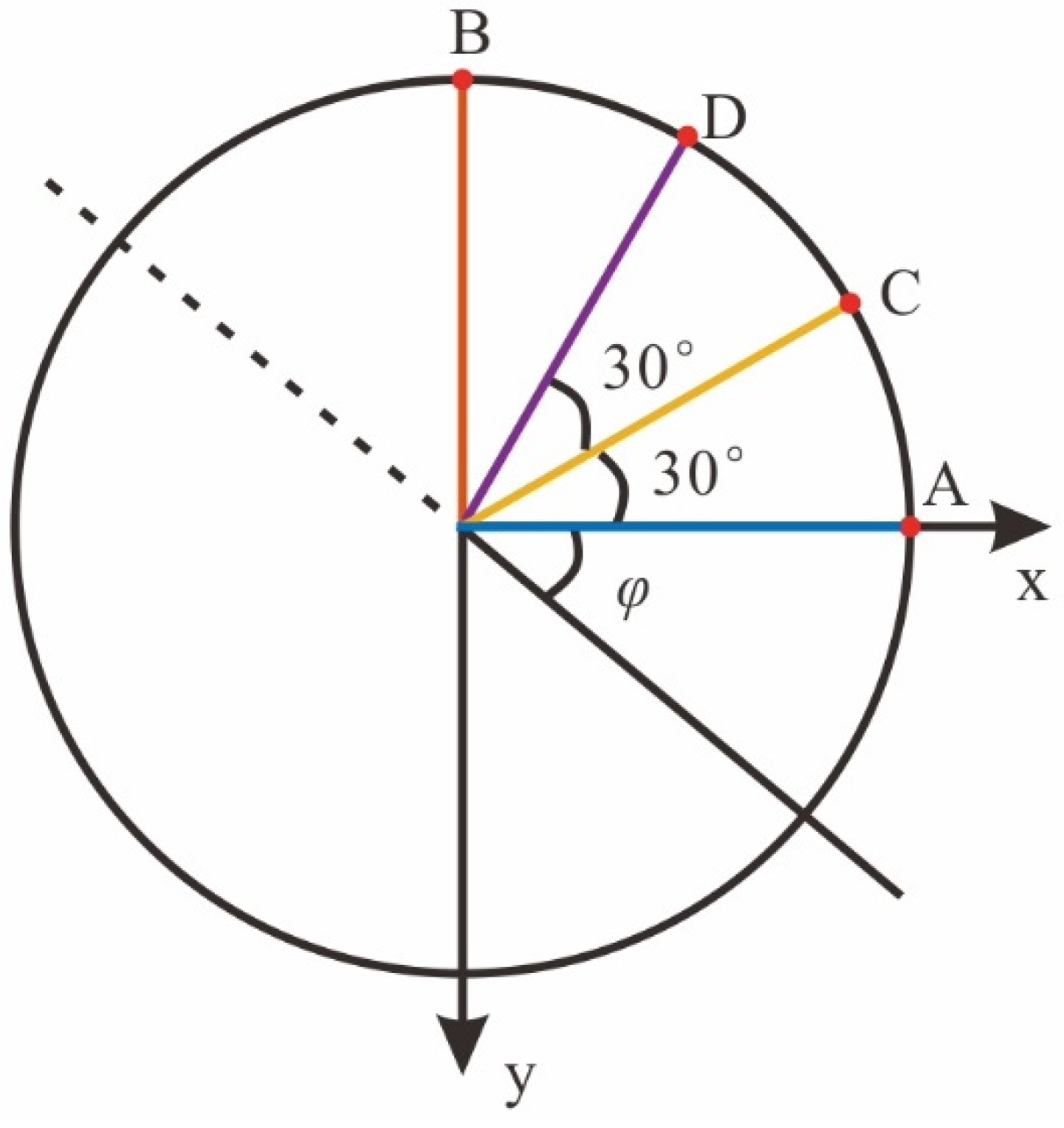
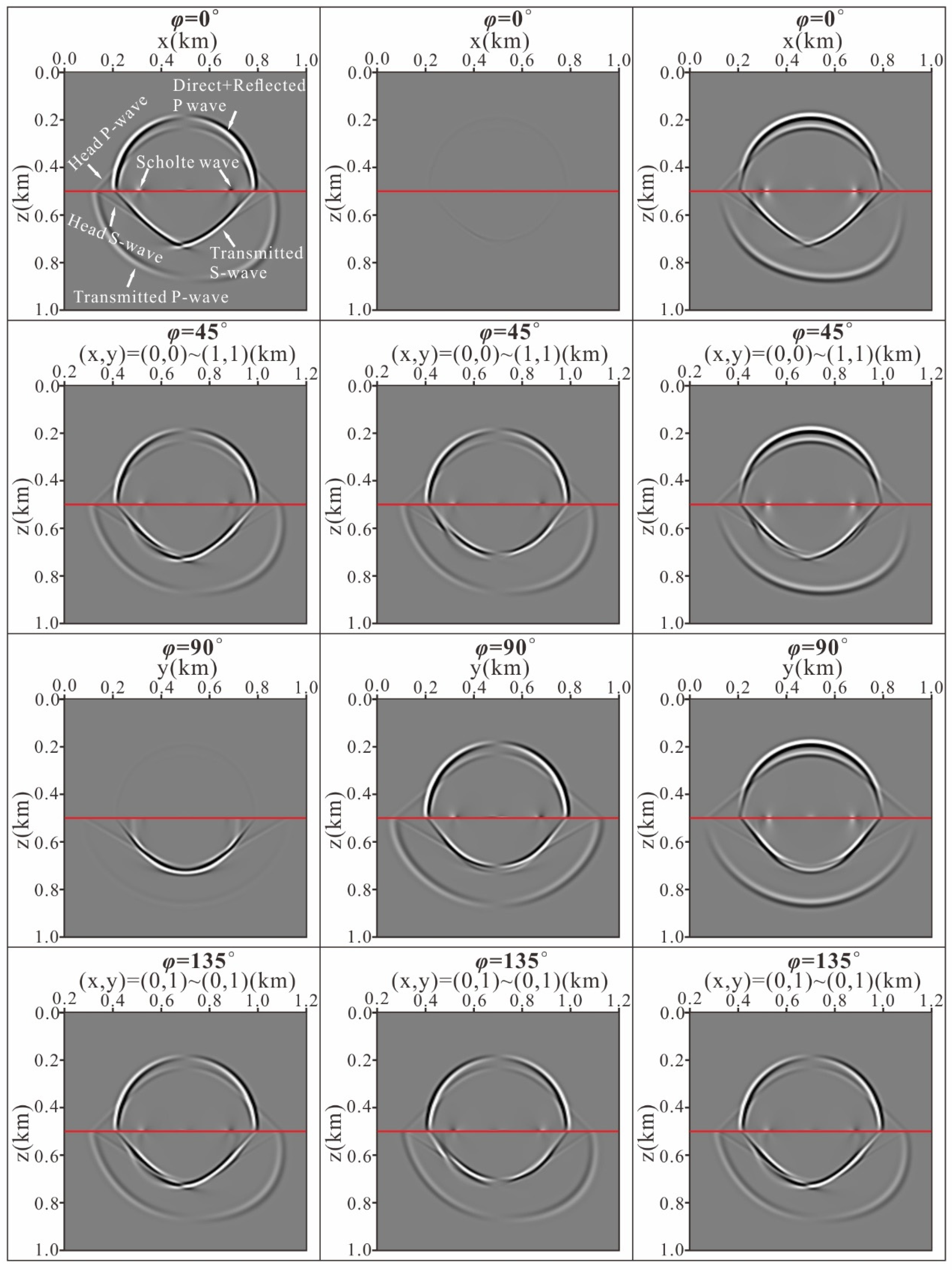
4.2. 3D Two-Layer Acoustic-Elastic Coupled Model

Second, we designed a 3D two-layer acoustic-elastic coupled model, where the upper and lower layer are fluid and TTI solid, respectively. The size of the model is $1 \mathrm{km}\times 1 \mathrm{km}\times 1 \mathrm{km}$. The grid spacing is $\Delta x=\Delta z=5\mathrm{m}$. The lower layer is defined by the Thomsen parameters: $V_{P0}=2.0 \mathrm{km}/\mathrm{s}$, $V_{S0}=1.1 \mathrm{km}/\mathrm{s}$, and the Thomsen parameters are $\epsilon =0.2$, $\delta =-0.05,$ and $\gamma =0.1$. The density of the lower layer is ${\rho }_S=1.5 {\mathrm{gcm}}^{-3}$. The acoustic velocity and density in the fluid are $V_f=1.5 \mathrm{km}/\mathrm{s}$ and ${\rho }_f=1.0 {\mathrm{gcm}}^{-3}$, respectively. A point source with 30 Hz wavelet is located at $\mathrm{x}=0.5 \mathrm{km}$, $\mathrm{y}=0.5 \mathrm{km},$ and $\mathrm{z}=0.48 \mathrm{km}$. The polar angle of the TTI symmetry axis is $\theta =45°$. The temporal step for the staggered-grid finite-difference method is $\Delta t=0.5 \mathrm{ms}$. We take observation lines as shown in Figure 8 and obtain the snapshots of different observation lines by numerical calculation (Figure 9). The parameter $\phi$ is the orientation of the observation line. Figure 9 shows that the wavefield snapshot includes the reflected/transmitted P wave, S wave, head wave, and the Scholte wave on the four tangent planes across the source projection point.

However, the velocity difference of the Scholte wave in different directions is not obvious. We set the polar angle $\theta$ to $0°$, $45°,$ and $90°$ to characterize the Scholte wave at the fluid-solid interface, respectively (Figure 10). We find that the velocity difference of the Scholte wave is obvious when the polar angle $\theta =90°$ (HTI); when the polar angle $\theta =0°$ (VTI), there is no velocity difference of the Scholte wave in different directions. The direct wave propagates in the isotropic water layer, and the reflection and transmission occur at the fluid-solid interface; the direct wave is circular.

We select four points on the fluid-solid interface (Figure 8) and record the time of Scholte waves arriving at the four points (Figure 11). The shape of the arrival time curve of the Scholte wave at point A is basically consistent with Figure 6; the peak at $\theta =45°$ disappears. The curve of point B is basically symmetric about $\theta =0°$. The curve of point C is close to the curve of point A. The curve of point D is close to the curve of point B. Figure 11 shows that the velocity of the Scholte wave at point B is positively related to the polar angle. When the polar angle $\theta =0°$, the curves intersect at one point. Scholte waves have the same velocity.

In this section, we apply the algorithm to a 3D homogeneous acoustic-elastic coupled model. We find that there is a difference in the velocity of Scholte waves when the polar angle θ changes. The curve of the Scholte wave arrival time has different motion trends with the change of polar angle θ in different orientations.

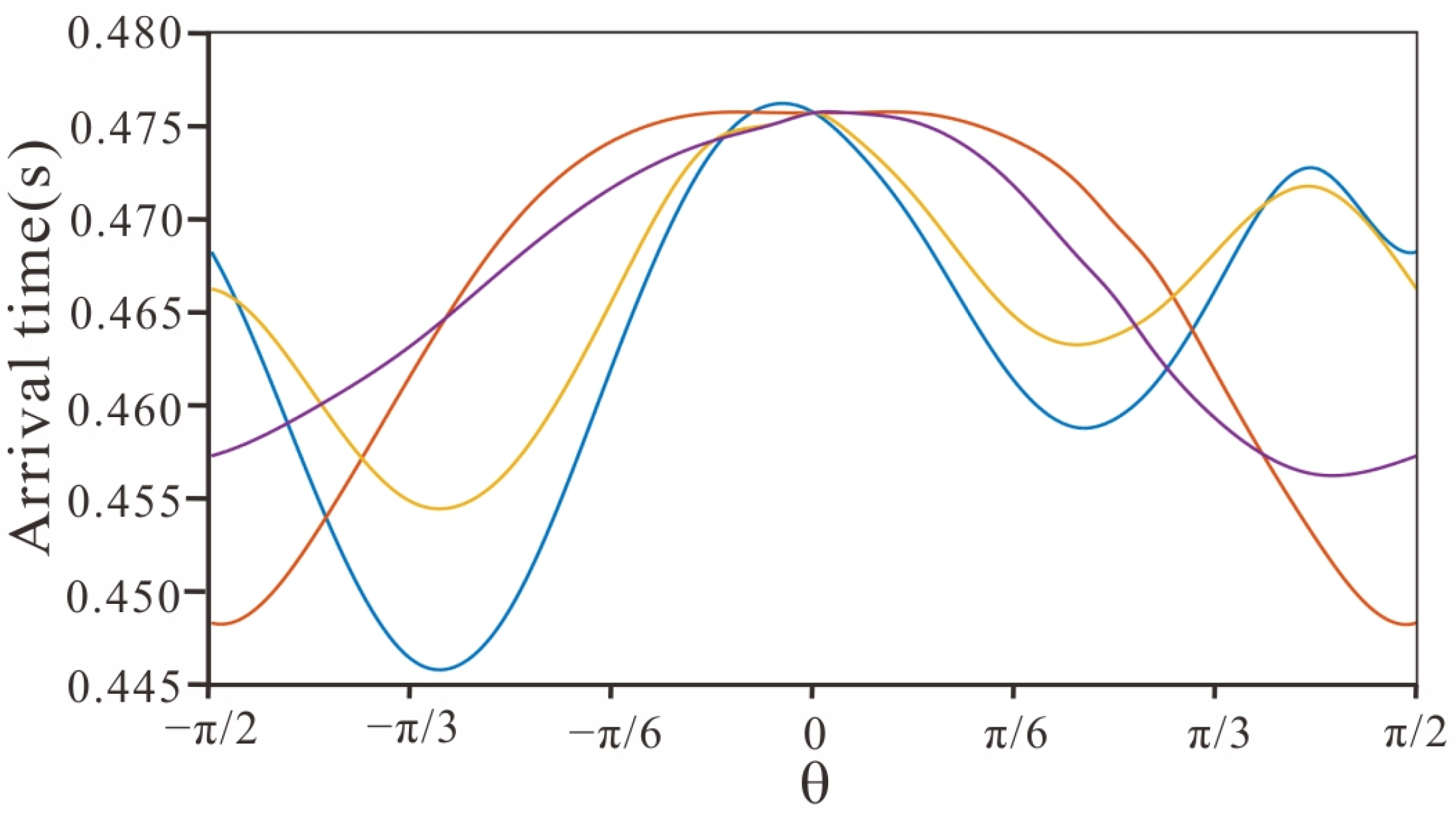
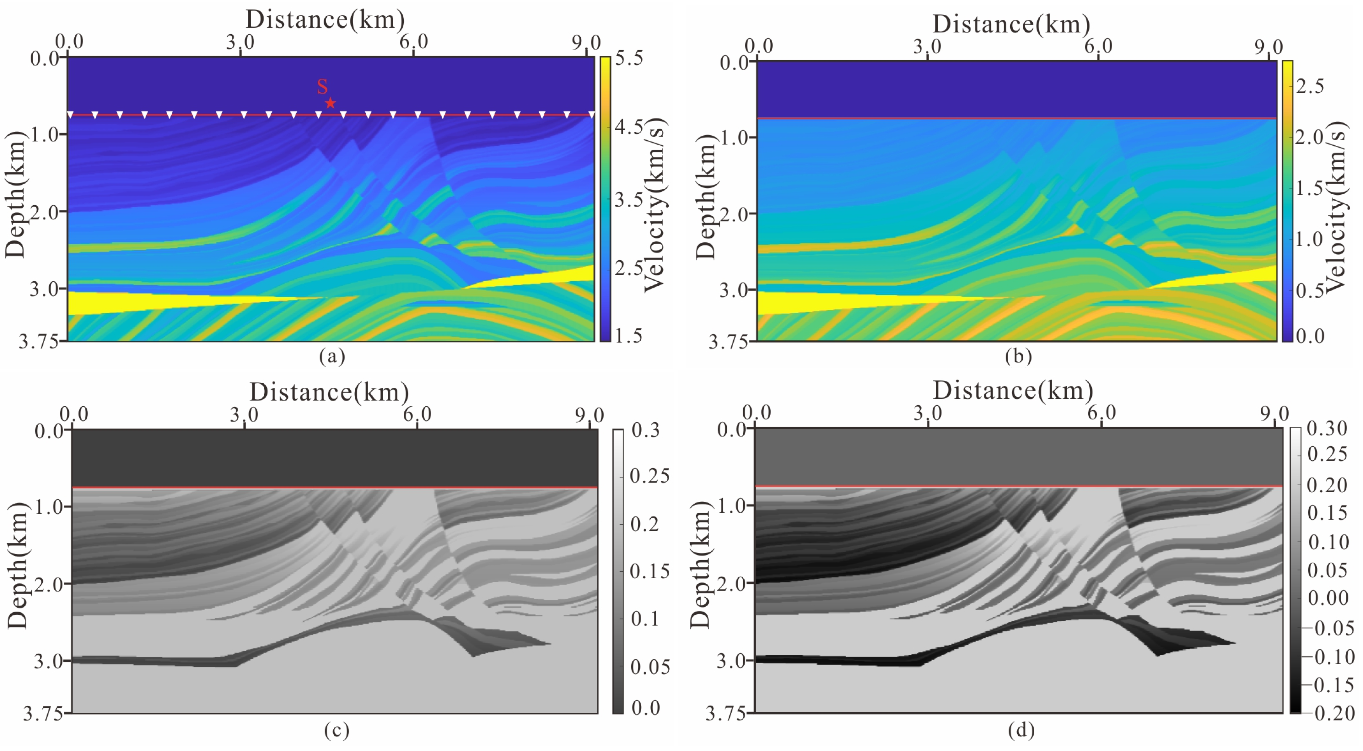
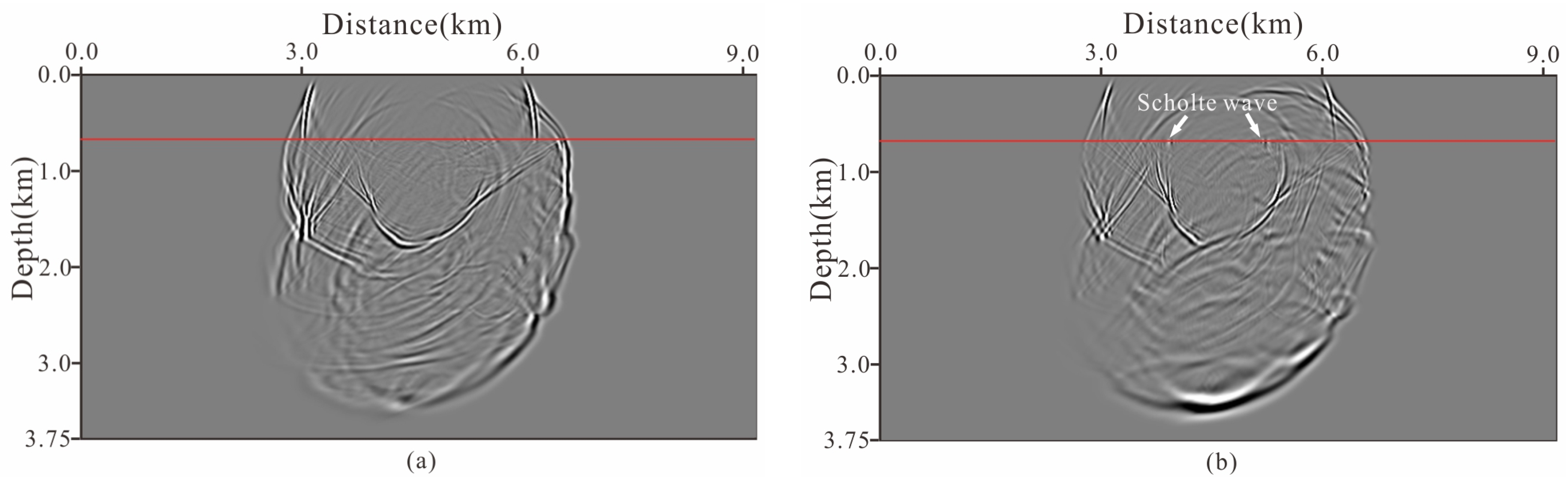
4.3. Inhomogeneous Acoustic-Elastic Coupled Model

The inhomogeneous TTI acoustic-elastic coupled media is shown in Figure 12, which is composed of the water layer and the inhomogeneous TTI media. The size of the model is $9.21 \mathrm{km}\times 3.75 \mathrm{km}$. The water layer is $0.75 \mathrm{km}$ thick. The grid spacing is $\Delta x=\Delta z=12.5\mathrm{m}$. The density of inhomogeneous TTI media is ${\rho }_S=1.8 {\mathrm{gcm}}^{-3}$, the polar angle $\theta$ is set to $-30°$, and the density of the fluid ${\rho }_f=1.0 {\mathrm{gcm}}^{-3}$. The temporal step for the staggered-grid finite-difference method is $\Delta t=1 \mathrm{ms}$. A point source with 20 Hz wavelet is located at $\mathrm{x}=4.62 \mathrm{km}$ and $\mathrm{z}=0.7375 \mathrm{km}$ (Figure 13).

Figure 13 shows the wavefield snapshots of the Marmousi-2 model. We can find that the snapshot of particle-velocity component $v_z$ includes the Scholte wave and body waves. Beside there is no dispersion in the calculation results. This indicates that our algorithm has fine stability and is suitable for complex models.

Without changing the transverse position, we gradually increase the distance between the source and the fluid-solid interface. The Scholte wave is clearly visible in the simulation results (Figure 14). It propagates along the horizontal fluid-solid interface, the time-distance curve is a straight line, and the velocity is lower than the minimum shear wave velocity of TTI media, which has strong propagation energy. When we reduce the distance between the source and the fluid-solid interface, the energy of the Scholte wave gradually decreases.

In this section, we apply the algorithm to the inhomogeneous acoustic-elastic coupled model. Numerical dispersion did not appear. This indicates that our algorithm is stable and can be applied to complex models. Moreover, we find that the distance between the source and the fluid-solid interface is negatively correlated with the energy of the Scholte wave.

5. Conclusions

We derive the 3D TTI acoustic-elastic coupled equations for controlling the wavefield propagation without considering complex boundary conditions. Through comparison with spectral element method, the effectiveness of our algorithm is proven, and it is suitable for the 3D space. The cost of this method is that compared with the acoustic equation, more parameters need to be set in the water layer, so the storage space and calculation time will be increased to a certain extent. Comparing curves from multiple sets of Thomsen parameters and polar angle $\theta$, we conclude that the velocity of the Scholte wave is positively correlated with $\epsilon$ and negatively correlated with $\delta$, and the curve of the arrival time of the Scholte wave is close to sinusoidal with respect to changes in the polar angle $\theta$. The results of the 3D model indicate that the velocity of the Scholte wave in the strike direction is positively related to the polar angle. The energy of the Scholte wave is negatively correlated with the distance from the source to the fluid-solid interface. This technology holds great potential in advancing marine seismic data imaging and Scholte wave research, especially in the exploration of renewable energy, providing a more cost-effective and accurate tool for the industry.

References

1. Miele, R.; Barreto, B.V.; Yamada, P.; Varella, L.E.S.; Pimentel, A.L.; Costa, J.F.; Azevedo, L. Geostatistical seismic rock physics AVA inversion with data-driven elastic properties update. IEEE Trans. Geosci. Remote Sens. 2021, 60, 4506915. [Google Scholar] [CrossRef]
2. Zhang, Y.; Zhao, H.; Yan, W.; Gao, J. A unified numerical scheme for coupled multiphysics model. IEEE Trans. Geosci. Remote Sens. 2020, 59, 8228–8240. [Google Scholar] [CrossRef]
3. Carcione, J.M.; Helle, H.B. The physics and simulation of wave propagation at the ocean bottom. Geophysics 2004, 69, 825–839. [Google Scholar] [CrossRef]
4. Shukla, K.; Carcione, J.M.; Hesthaven, J.S.; L’heureux, E. Waves at a fluid-solid interface: Explicit versus implicit formulation of boundary conditions using a discontinuous Galerkin method. J. Acoust. Soc. Am. 2020, 147, 3136–3150. [Google Scholar] [CrossRef]
5. Kovářík, K.; Mužík, J. The Modified Local Boundary Knots Method for Solution of the Two-Dimensional Advection–Diffusion Equation. Mathematics 2022, 10, 3855. [Google Scholar] [CrossRef]
6. Kovářík, K.; Mužík, J.; Gago, F.; Sitányiová, D. Modified local singular boundary method for solution of two-dimensional diffusion equation. Eng. Anal. Bound. Elem. 2022, 143, 525–534. [Google Scholar] [CrossRef]
7. Li, C.; Wang, Y.; Zhang, J.; Geng, J.; You, Q.; Hu, Y.; Liu, Y.; Hao, T.; Yao, Z. Separating Scholte Wave and Body Wave in OBN Data Using Wave-Equation Migration. IEEE Trans. Geosci. Remote Sens. 2022, 60, 5914213. [Google Scholar] [CrossRef]
8. Zhan, G.; Pestana, R.C.; Stoffa, P.L. Decoupled equations for reverse time migration in tilted transversely isotropic media. Geophysics 2012, 77, T37–T45. [Google Scholar] [CrossRef]
9. Zdraveva, O.; Ogunsakin, A.; Hootman, B.; Kristiansen, P.; Quadt, E. Improved imaging of deepwater reservoir by TTI model building and optimized use of OBN data: 85th SEG Annual International Meeting. In Expanded Abstracts; Society of Exploration Geophysicists: Houston, TX, USA, 2015; pp. 5198–5201. [Google Scholar] [CrossRef]
10. Qu, Y.; Li, J.; Li, Y.; Li, Z. Joint acoustic and decoupled-elastic least-squares reverse time migration for simultaneously using water-land dual-detector data. IEEE Trans. Geosci. Remote Sens. 2023, 61, 5909511. [Google Scholar] [CrossRef]
11. Lan, T.; Zong, Z.; Jia, W. Reservoir hydrocarbon identification method based on pre-stack seismic frequency-dependent anisotropic inversion. IEEE Trans. Geosci. Remote Sens. 2023, 61, 5915413. [Google Scholar] [CrossRef]
12. Cagniard, L.; Flinn, E.A.; Hewitt Dix, C.; Mayer, W.G. Reflection and refraction of progressive seismic waves. Phys. Today 1963, 16, 64. [Google Scholar] [CrossRef]
13. Carbajal-Romero, M.; Flores-Mendez, E.; Flores-Guzmán, N.; Núñez-Farfán, J.; Olivera-Villaseñor, E.; Sánchez-Sesma, F.J. Scholte waves on fluid-solid interfaces by means of an integral formulation. Geofís. Int. 2013, 52, 21–30. [Google Scholar] [CrossRef]
14. van Vossen, R.; Robertsson, J.O.; Chapman, C.H. Finite-difference modeling of wave propagation in a fluid-solid configuration. Geophysics 2002, 67, 618–624. [Google Scholar] [CrossRef]
15. Zhao, S.; Zhang, J.; Wang, Z.; Huang, H.; Hu, J.; Guo, C.a. Improving Scholte-Wave vibration signal recognition based on polarization characteristics in coastal waters. J. Coast. Res. 2020, 36, 382–392. [Google Scholar] [CrossRef]
16. Xin, X.; Yong-Ge, W.; Zhen-Yue, L.; Shu-Zhong, S. Scholte wave dispersion and particle motion mode in ocean and ocean crust. Appl. Geophys. 2022, 19, 132–142. [Google Scholar] [CrossRef]
17. Wang, W.; Mokhtari, A.A.; Srivastava, A.; Amirkhizi, A.V. Angle-dependent phononic dynamics for data-driven source localization. J. Acoust. Soc. Am. 2023, 154, 2904–2916. [Google Scholar] [CrossRef] [PubMed]
18. Auld, B. Rayleigh wave propagation. In Rayleigh-Wave Theory and Application, Proceedings of the International Symposium Organised by the Rank Prize Funds at the Royal Institution, London, UK, 15–17 July 1985; Springer: Berlin/Heidelberg, Germany, 1985; pp. 12–27. [Google Scholar]
19. Carcione, J.M.; Bagaini, C.; Ba, J.; Wang, E.; Vesnaver, A. Waves at fluid–solid interfaces: Explicit versus implicit formulation of the boundary condition. Geophys. J. Int. 2018, 215, 37–48. [Google Scholar] [CrossRef]
20. Glorieux, C.; Van de Rostyne, K.; Gusev, V.; Gao, W.; Lauriks, W.; Thoen, J. Nonlinearity of acoustic waves at solid–liquid interfaces. J. Acoust. Soc. Am. 2002, 111, 95–103. [Google Scholar] [CrossRef]
21. Glorieux, C.; Van de Rostyne, K.; Nelson, K.; Gao, W.; Lauriks, W.; Thoen, J. On the character of acoustic waves at the interface between hard and soft solids and liquids. J. Acoust. Soc. Am. 2001, 110, 1299–1306. [Google Scholar] [CrossRef]
22. Padilla, F.; de Billy, M.; Quentin, G. Theoretical and experimental studies of surface waves on solid–fluid interfaces when the value of the fluid sound velocity is located between the shear and the longitudinal ones in the solid. J. Acoust. Soc. Am. 1999, 106, 666–673. [Google Scholar] [CrossRef]
23. Lee, H.-Y.; Lim, S.-C.; Min, D.-J.; Kwon, B.-D.; Park, M. 2D time-domain acoustic-elastic coupled modeling: A cell-based finite-difference method. Geosci. J. 2009, 13, 407–414. [Google Scholar] [CrossRef]
24. Bernth, H.; Chapman, C. A comparison of the dispersion relations for anisotropic elastodynamic finite-difference grids. Geophysics 2011, 76, WA43–WA50. [Google Scholar] [CrossRef]
25. Cao, J.; Brossier, R.; Górszczyk, A.; Métivier, L.; Virieux, J. 3-D multiparameter full-waveform inversion for ocean-bottom seismic data using an efficient fluid–solid coupled spectral-element solver. Geophys. J. Int. 2022, 229, 671–703. [Google Scholar] [CrossRef]
26. Di Bartolo, L.; Manhisse, R.R.; Dors, C. Efficient acoustic-elastic FD coupling method for anisotropic media. J. Appl. Geophys. 2020, 174, 103934. [Google Scholar] [CrossRef]
27. Qu, Y.; Huang, J.; Li, Z.; Li, J. A hybrid grid method in an auxiliary coordinate system for irregular fluid-solid interface modeling. Geophys. J. Int. 2016, 208, 1540–1556. [Google Scholar] [CrossRef]
28. Li, Q.; Wu, G.; Jia, Z.; Duan, P. Full-waveform inversion in acoustic-elastic coupled media with irregular seafloor based on the generalized finite-difference method. Geophysics 2023, 88, T83–T100. [Google Scholar] [CrossRef]
29. Sethi, H.; Shragge, J.; Tsvankin, I. Tensorial elastodynamics for coupled acoustic/elastic anisotropic media: Incorporating bathymetry. Geophys. J. Int. 2022, 228, 999–1014. [Google Scholar] [CrossRef]
30. Fornberg, B. The pseudospectral method; accurate representation of interfaces in elastic wave calculations. Geophysics 1988, 53, 625–637. [Google Scholar] [CrossRef]
31. Komatitsch, D.; Barnes, C.; Tromp, J. Wave propagation near a fluid-solid interface: A spectral-element approach. Geophysics 2000, 65, 623–631. [Google Scholar] [CrossRef]
32. Sun, M.; Jin, S.; Yu, P. Elastic least-squares reverse-time migration based on a modified acoustic-elastic coupled equation for OBS four-component data. IEEE Trans. Geosci. Remote Sens. 2021, 59, 9772–9782. [Google Scholar] [CrossRef]
33. Yu, P.; Geng, J.; Li, X.; Wang, C. Acoustic-elastic coupled equation for ocean bottom seismic data elastic reverse time migration. Geophysics 2016, 81, S333–S345. [Google Scholar] [CrossRef]
34. Yu, P.; Geng, J.; Wang, C. Separating quasi-P-wave in transversely isotropic media with a vertical symmetry axis by synthesized pressure applied to ocean-bottom seismic data elastic reverse time migration. Geophysics 2016, 81, C295–C307. [Google Scholar] [CrossRef]
35. Yu, P.; Geng, J. Acoustic-elastic coupled equations in vertical transverse isotropic media for pseudoacoustic-wave reverse time migration of ocean-bottom 4C seismic data. Geophysics 2019, 84, S317–S327. [Google Scholar] [CrossRef]
36. Han, L.; Huang, X.; Hao, Q.; Greenhalgh, S.; Liu, X. Incorporating the nearly constant Q models into 3-D poro-viscoelastic anisotropic wave modeling. IEEE Trans. Geosci. Remote Sens. 2023, 61, 4501811. [Google Scholar] [CrossRef]
37. He, X.; Yang, D.; Huang, J.; Huang, X. Modeling 3-D Elastic Wave Propagation in TI Media Using Discontinuous Galerkin Method on Tetrahedral Meshes. IEEE Trans. Geosci. Remote Sens. 2023, 61, 5904514. [Google Scholar] [CrossRef]
38. Mathewson, J.; Bachrach, R.; Ortin, M.; Decker, M.; Kainkaryam, S.; Cegna, A.; Paramo, P.; Vincent, K.; Kommedal, J. Offshore Trinidad tilted orthorhombic imaging of full-azimuth OBC data. In Proceedings of the SEG International Exposition and Annual Meeting, New Orleans, LA, USA, 18–23 October 2015; p. SEG–2015-5848590. [Google Scholar]
39. Xie, Y.; Zhou, B.; Zhou, J.; Hu, J.; Xu, L.; Wu, X.; Lin, N.; Loh, F.C.; Liu, L.; Wang, Z. Orthorhombic full-waveform inversion for imaging the Luda field using wide-azimuth ocean-bottom-cable data. Lead. Edge 2017, 36, 75–80. [Google Scholar] [CrossRef]
40. Raymer, D.; Kendall, J.; Pedlar, D.; Kendall, R.; Mueller, M.; Beaudoin, G. The significance of salt anisotropy in seismic imaging. In Proceedings of the SEG International Exposition and Annual Meeting, Online, 11–16 October 2000; p. SEG–2000-0562. [Google Scholar]
41. Hao, Q.; Stovas, A. The offset-midpoint travel-time pyramid for P-wave in 2D transversely isotropic media with a tilted symmetry axis. Geophys. Prospect. 2015, 63, 587–596. [Google Scholar] [CrossRef]
42. Zeighami, F.; Quqa, S.; De Ponti, J.M.; Ayyash, N.; Marzani, A.; Palermo, A. Elastic metasurfaces for Scholte–Stoneley wave control. Philos. Trans. A 2024, 382, 20230365. [Google Scholar] [CrossRef]
43. DONG, L.G.; MA, Z.T.; CAO, J.Z. Stability of the staggered-grid high-order difference method for first-order elastic wave equation. Chin. J. Geophys. 2000, 43, 904–913. [Google Scholar]
44. Igel, H.; Mora, P.; Riollet, B. Anisotropic wave propagation through finite-difference grids. Geophysics 1995, 60, 1203–1216. [Google Scholar] [CrossRef]
45. Koene, E.F.; Robertsson, J.O.; Broggini, F.; Andersson, F. Eliminating time dispersion from seismic wave modeling. Geophys. J. Int. 2018, 213, 169–180. [Google Scholar] [CrossRef]
46. Wang, Y.; Liang, W.; Nashed, Z.; Li, X.; Liang, G.; Yang, C. Seismic modeling by optimizing regularized staggered-grid finite-difference operators using a time-space-domain dispersion-relationship-preserving method. Geophysics 2014, 79, T277–T285. [Google Scholar] [CrossRef]
47. Komatitsch, D.; Vilotte, J.-P. The spectral element method: An efficient tool to simulate the seismic response of 2D and 3D geological structures. Bull. Seismol. Soc. Am. 1998, 88, 368–392. [Google Scholar] [CrossRef]
Figure 1. Coordinate transformation diagram of Bond matrix.
Applsci 14 08302 g001
Figure 2. 3D staggered grid and parameter definition diagram. The stresses and the pressure field are defined at the standard grid points. The velocity components and Thomsen parameters of the acoustic-elastic coupled media are defined on the staggered grid points.
Applsci 14 08302 g002
Figure 3. Snapshots of particle-velocity components (a) v x and (b) v z at t = 0.5   s . The red line denotes the fluid-solid interface.
Applsci 14 08302 g003
Figure 4. Snapshots of particle-velocity components (a) v x and (b) v z with spectral element method at t = 0.5   s . The red line denotes the fluid-solid interface.
Applsci 14 08302 g004
Figure 5. The vibration curve of the Scholte wave.
Applsci 14 08302 g005
Figure 6. Arrival time of the Scholte wave with a different polar angle.
Applsci 14 08302 g006
Figure 7. Arrival time of the Scholte wave with different Thomsen parameters (a) ε and (b) δ. In plot (a) δ = 0.05 , θ = 30 ° ; In plot (b) ε = 0.2 , θ = 30 ° .
Applsci 14 08302 g007
Figure 8. The orientation of the observation line. φ denotes the orientation of the observation line. The points are used to test the arrival time of the Scholte wave.
Applsci 14 08302 g008
Figure 9. Snapshots of the components (left) v x , (centre) v y , and (right) v z at t = 0.25   s . The red line denotes the fluid-solid interface. The plane of parameter φ = 0 ° is XOZ plane, and the plane of parameter φ = 90 ° is YOZ plane. The Thomsen parameters are ε = 0.2 , δ = 0.05 , and γ = 0.1 .
Applsci 14 08302 g009
Figure 10. Snapshots of the components (left) v x , (centre) v y , and (right) v z on the fluid-solid interface at t = 0.25   s . The Thomsen parameters are ε = 0.2 , δ = 0.05 and γ = 0.1 .
Applsci 14 08302 g010
Figure 11. Arrival time of the Scholte wave at point A, B, C, and D with different polar angles. The blue, red, yellow, and purple lines are point A, B, C, and D, respectively. The Thomsen parameters are ε = 0.2 , δ = 0.05 , and γ = 0.1 .
Applsci 14 08302 g011
Figure 12. Acoustic-elastic coupled Marmousi-2 model. Plots (ad) are the P- and SV-wave vertical velocities and the Thomsen parameters ε and δ , respectively. The red line is the fluid-solid interface. The icon S represents the point source.
Applsci 14 08302 g012
Figure 13. Snapshots of particle-velocity components (a) v x and (b) v z at t = 1.1   s . The red line denotes the fluid-solid interface.
Applsci 14 08302 g013
Figure 14. Seismograms from the Marmousi2 model. The water layer is 0.75   km thick. (a): The source is located at x = 4.62   km and z = 0.7375   km ; (b): The source is located at x = 4.62   km and z = 0.725   km ; (c): The source is located at x = 4.62   km and z = 0.7   km .
Applsci 14 08302 g014aApplsci 14 08302 g014b