Article

Examining the Optimization of Spray Cleaning Performance for LiDAR Sensor

1
Department of Future Vehicle Research, Korea Automobile Testing and Research Institute, Hwaseong 18247, Republic of Korea
2
TOD Based Transportation Research Center, Ajou University, Suwon 16499, Republic of Korea
3
Department of Advanced Development, SL Co., Ltd., Daegu 41514, Republic of Korea
4
Department of Artificial Intelligence Convergence, Sahmyook University, Seoul 01795, Republic of Korea
*
Author to whom correspondence should be addressed.
Appl. Sci. 2024, 14(18), 8340; https://doi.org/10.3390/app14188340
Submission received: 27 July 2024 / Revised: 9 September 2024 / Accepted: 13 September 2024 / Published: 16 September 2024

Abstract

:
Pollutants degrade the performance of LiDAR sensors used in autonomous vehicles. Therefore, there is an urgent need to develop cleaning technology for these sensors. In this study, a solid-state LiDAR sensor was selected as a target and sprayed/dried with 2.5 g of a mixture of Arizona dust and Kaolin. To achieve optimal LiDAR cleaning performance, the washer pressure, spray time, spray angle, and target point were selected as major variables. Additionally, an optimal cleaning solution for each spray was formed via the design of experiments and optimization techniques. Model suitability was observed for the second spray through to the fourth. The cleaning rate increased with the washer pressure and spray time. The influence of these variables decreased as the number of sprays increased. The spray angle and target point exhibited no significant influence, but excellent cleaning was observed in some central areas. Verification test results were within 3% for the second through fourth sprays, indicating reliability. This study used a designed experiment with 30 scenarios to reveal optimized conditions for protecting the sensor performance from external visibility obstructions. Disclosing the optimization method lowers the barrier for sensor cleaning manufacturers to develop their own technology, which ultimately enhances safer and more efficient autonomous driving.

1. Introduction

The rapid advancement of autonomous driving technology promotes the idea of a future of self-driven vehicles. Considerable efforts toward the research and development of this technology have been made, owing to the potential benefits of autonomous vehicles, such as improvements in road safety, traffic flow, and accessibility.
The production of vehicles with level-3 autonomous driving technology has begun, while aggressive research and developmental works are underway by governments and manufacturers toward level-4 technology. Numerous global manufacturers, including Tesla, Waymo, GM, Audi, Valeo, Hyundai Motor Company, and NVIDIA, have launched vehicles equipped with autonomous driving technology. Autonomous vehicles collect real-time data on the surrounding environment using various sensors including light detection and ranging (LiDAR), radar, cameras, and ultrasonic sensors. This is the fundamental process by which a vehicle can properly search, respond, and make instant decisions regarding unexpected obstacles. However, the accuracy and performance of the sensors can be adversely affected by pollutants, such as dust, rain, and snow, that accumulate on them or by various other environmental factors. Sensor performance degradation can cause potentially dangerous situations through inaccurate data recognition.
Several studies have been conducted to address the performance degradation of sensors used in autonomously driven vehicles that is caused by environmental pollutants, such as snow, dust, sand, and mud. Technologies to detect vehicles in inclement weather data sets [1], research on generative adversarial networks to remove raindrops from single images [2], and technologies to restore images through de-raining [3] exist. Various studies have focused on solving cognitive degradation caused by external environmental factors through image-filtering algorithms [4]. Additionally, a study was conducted on the recognition rate through dust synthesis in a virtual camera scenario [5]. Hyundai Motor Company is set to mass-produce camera sensor cleaning systems while developing their Rotator-Cam technology for level-4 autonomous driving [6]. XenomatiX has established a partnership with Kautex Clear Vision Systems to develop LiDAR-suitable cleaning solutions for adverse weather and cover contamination [7]. Furthermore, premium vehicles, such as the BMW 7 Series and Mercedes S-Class, which feature cleaning systems for some of their sensors, demonstrate the importance of maintaining sensor accuracy under all environmental conditions [8,9]. Research on technologies to detect foreign substances on sensors [10] is urgently required along with the development of innovative solutions to ensure consistent and stable data collection for autonomous driving systems by optimizing sensor cleaning technology.
This study developed an optimized cleaning technological design method for LiDAR sensors that use light [11] instead of radar with relatively high permeability. Among several sensors used in autonomous driving technology, LiDAR sensors that had been affected by external foreign substances that degrade their performance were selected through the design of experiments (DOE) method. Various types of LiDAR sensors were examined to select a target sensor, and a solid-state LiDAR sensor (manufacture: AutoL, Model name: G32) that is more highly evaluated than mechanical LiDAR sensors in terms of design was selected. Based on an existing study [12], a sample to reproduce strong dust was prepared by mixing Arizona dust (ARI) and Kaolin (KL) with 50% water. An amount of 2.5 g of the sample was sprayed and dried. The washer pressure, spray time, spray angle, and target point were selected as the main factors for cleaning optimization. A total of 30 standard experimental targets were selected through DOE.
Washer spraying is essential for sensor cleaning, and additional methods, such as air jets, wipers, and electrical systems, have been used to remove residual washer fluid and foreign substances after spraying [13]. In this study, the washer spraying method was chosen as the primary cleaning method to determine the optimal spray conditions.
This paper discusses the optimal washer sensor cleaning technology applicable to the autonomous driving industry and presents an optimal, comprehensive, and applicable solution. When applied to cleaning prototypes used in future autonomous vehicles, the results of this study are expected to lower entry barriers to development for related technological developers and contribute to the spread of safer technological applications. In this study, we developed optimization methods that were specific to LiDAR sensors and did not consider the influence of airflow [14]. Therefore, a commonly used nozzle type was selected to produce representative results that can be applied to a variety of LiDAR sensors. The experiment on optimization technology for the LiDAR sensor and the disclosure of all analytical approaches effectively reduce the time and cost required for the development of optimization technology.
This paper is structured into four main sections: Section 2 details the materials and methodologies used, the specific conditions and procedures are presented in Appendix A.1, Section 3 presents and analyzes the findings in context with existing research, and, finally, Section 4 summarizes the key findings of this study and their implications and suggests future research directions.

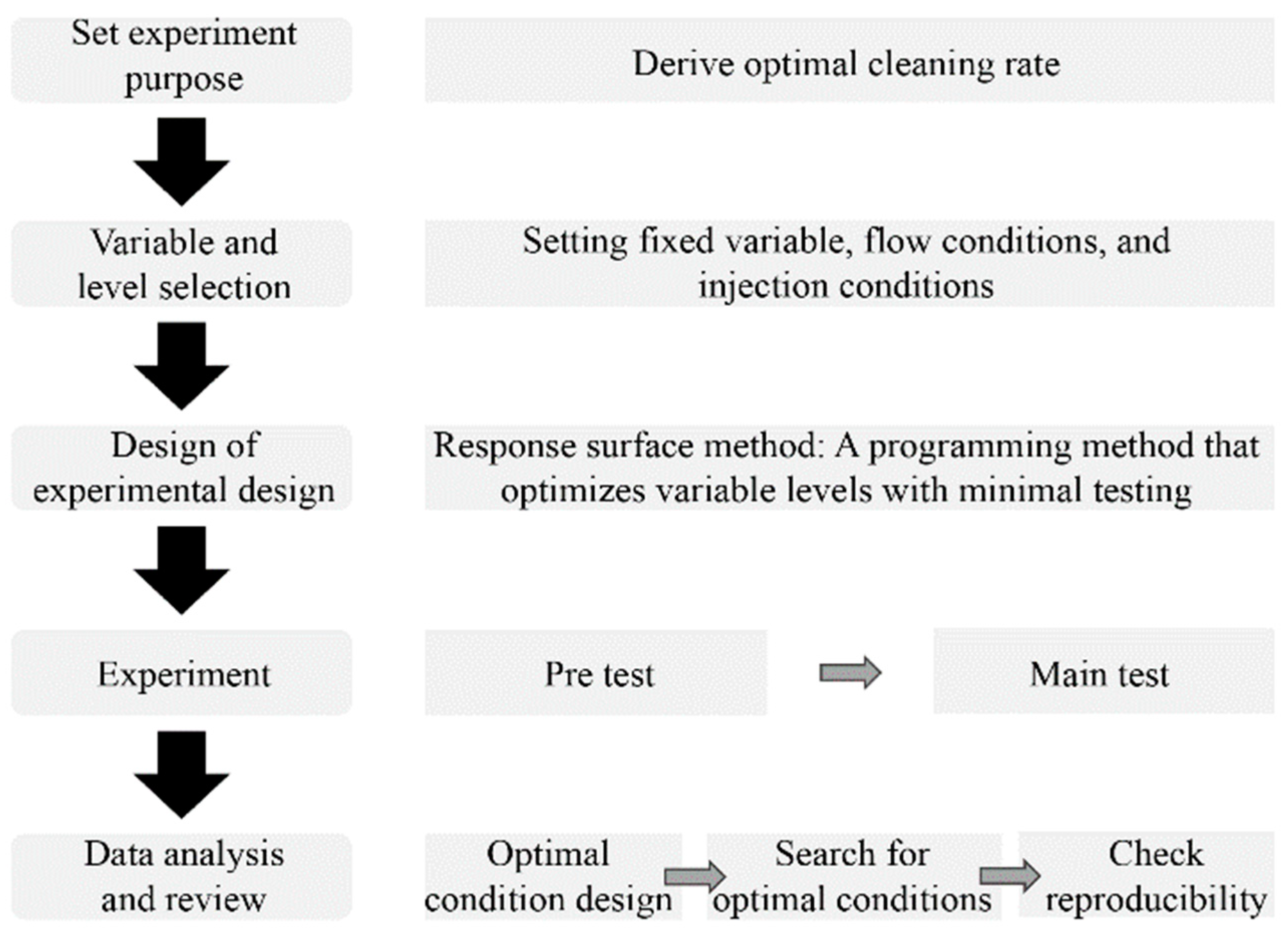
2. Materials and Methods

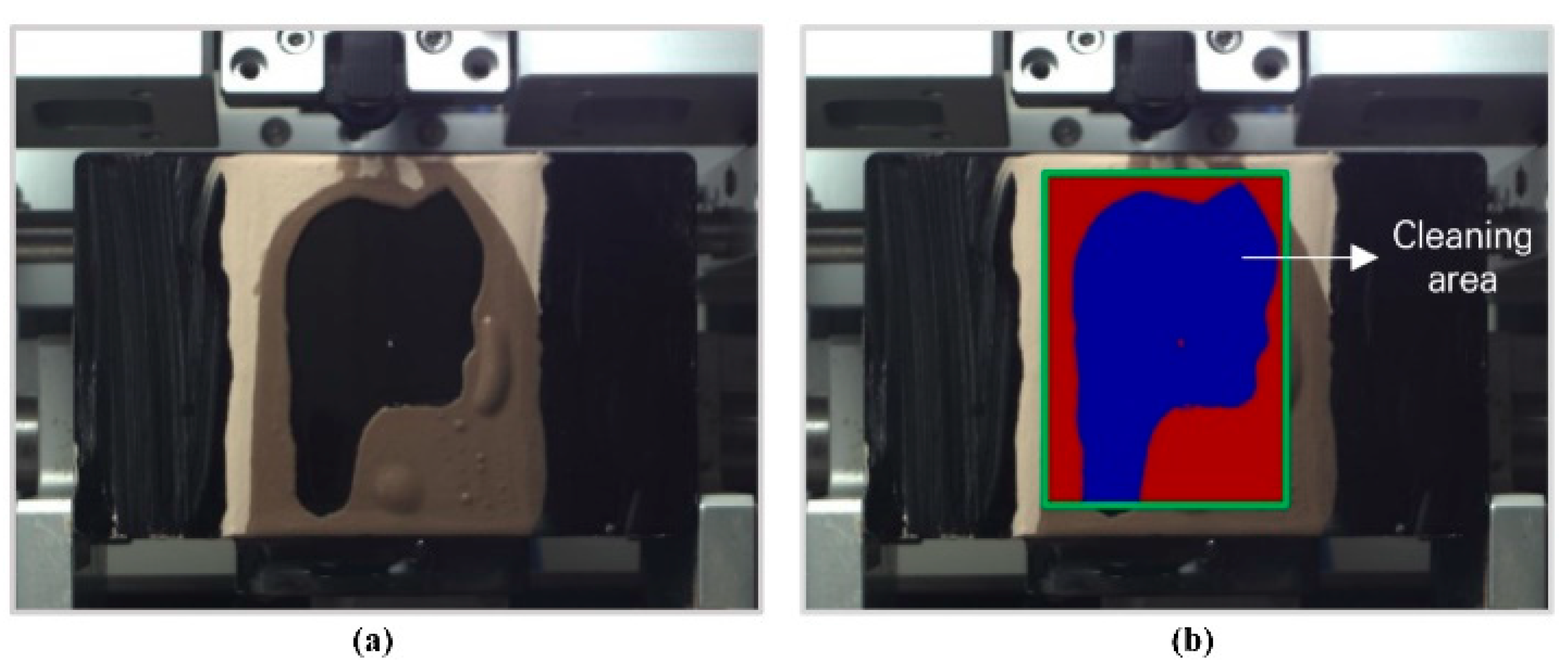
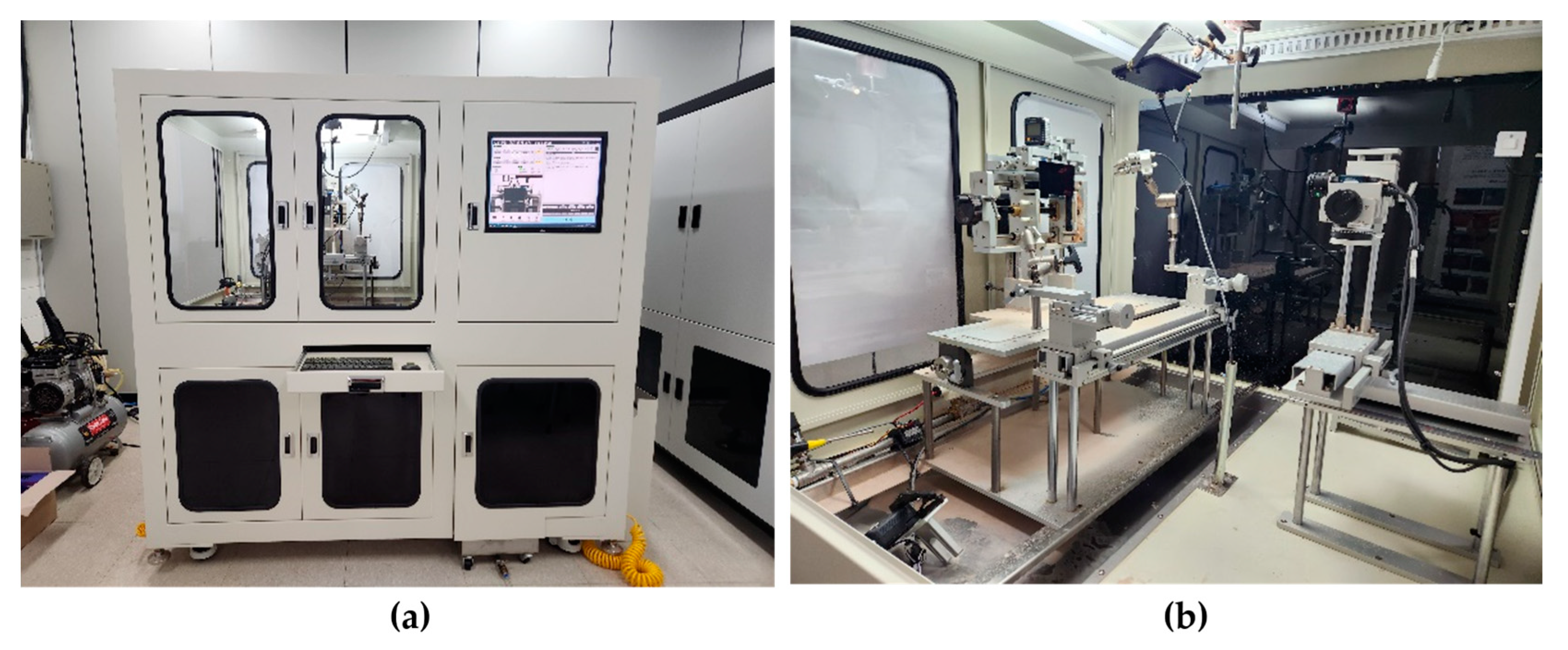
2.1. Blockage Cleaning Test Bench

Blockage cleaning test bench(Techways, Yongin, Republic of Korea) is a system developed for conducting experiments on cleaning capability optimization by placing a contaminated sensor on a test bench sensor mount, as shown in Figure 1. The system is designed to evaluate cleaning ability by equipping various LiDAR sensors and adjusting the main cleaning elements, such as washer pressure, spray angle, spray time, and target point [15,16]. The front section was designed to fix the LiDAR window cover at the center, and the injection angle of the washer nozzle was adjusted. The targeted point was adjusted along the vertical direction.
Figure 2a shows an overall view of the equipment, whereas Figure 2b shows the inside view. After mounting the LiDAR with its window covered in dust, photographs were captured using a camera before and after cleaning. Thereafter, the cleaning rate was automatically calculated using the images and analyzer.

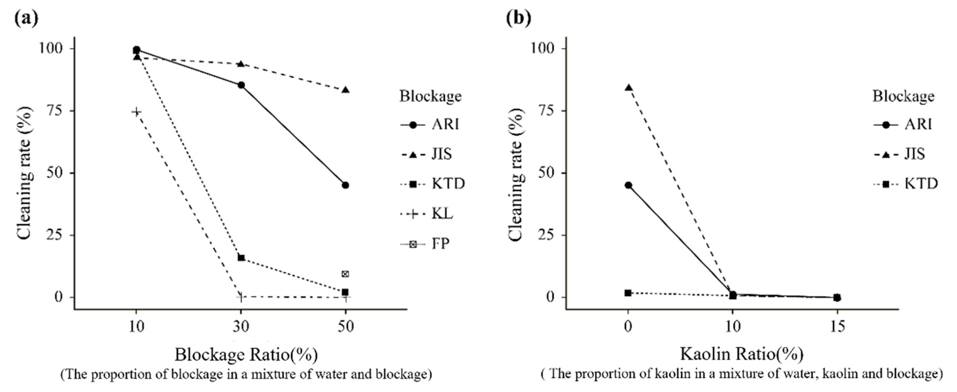
2.2. Research on Experimental Blockage

Blockage types were largely divided into dust, biological, and meteorological factors. In a previous study [13], dust was used to evaluate the performance of windshield wipers in ordinary vehicles according to the ARI test and Japanese Industrial Standards (JIS, Kawasaki, Japan). KL (Jiangxi, China), used to make ceramics and cement (hereafter PT, ME, USA) for road and facility constructions, was also incorporated as an additive. Dust affected the blockage performance depending on its dryness and water concentration. Figure 3 shows the cleaning rate results under different conditions according to the blockage type. Here, KTD (Gochang, Republic of Korea) represents Korean test dust, and FP represents fake poop.
As shown in Figure 3a, all dust types exhibited similar cleaning rates, excluding KL at a dust concentration of 10%. As the concentration increased to 30 and 50%, different characteristics were observed. JIS shows no significant difference with change in concentration, whereas ARI exhibited large differences. For KTD and KL, the cleaning rate rapidly decreased from 30% and was lower than that of FP at 50%.
Figure 3b shows the performance results when KL was added to the three dust types, ARI, JIS, and KTD. With the addition of KL, blockage production with higher performance was possible because KL was highly viscous, and it increased adhesion when sprayed onto the LiDAR window cover. In this study, the aforementioned dust characteristics were considered, and an optimal test dust was derived by combining ARI and KL, which have been widely used in numerous dust tests.

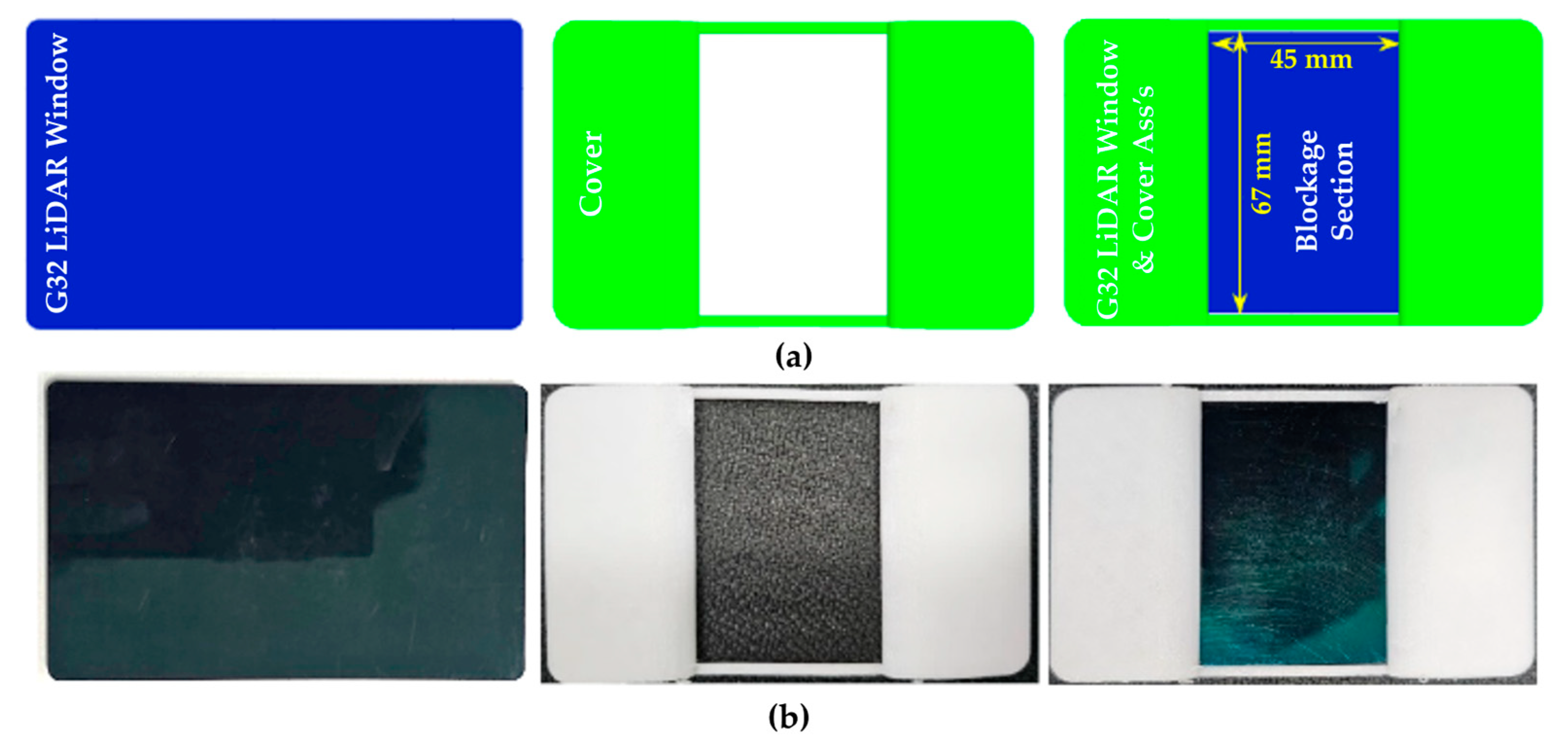
2.3. Selection of Target LiDAR and Window Cover Sample

2.3.1. Selection of Target LiDAR

A developed and mass-produced LiDAR for vehicles was selected to secure the reliability of the test. The G32 model from AutoL(Seongnam, Republic of Korea) was selected for evaluation considering the trend and test suitability of the solid-state LiDAR, which offered benefits in terms of design. Figure 4 shows the exterior of the selected LiDAR, whereas its detailed specifications are listed in Table 1.

2.3.2. Window Cover Sample

The selected LiDAR had dimensions of 107 mm × 67 mm × 3 mm (length × height × width), as shown in Figure 5.
The entire window area of the G32 LiDAR was divided into two zones, the laser transmitter and receiver areas located in the red A and yellow B zones, respectively. Figure 6 shows the window section where the transmitter and receiver areas were located.
The laser transmitter of the target LiDAR was located at its center, as shown in Figure 6. The contamination of the LiDAR sensor due to the blockage of its transceiver area could be fatal and detrimental to autonomous driving safety. Additionally, the washer nozzle should be installed considering the optimal position for cleaning the LiDAR transmitter and the influence of the washer nozzle on the field of view (FOV) of the LiDAR. In this study, the nozzle was placed at the center of the LiDAR window by measuring the trajectory of the liquid injected by the washer. To derive washer system design parameters that represent the optimal cleaning rate, the washer pressure, spray time, spray angle, and target point were selected as major variables.

2.3.3. Dust Spray Guide

The entire area of the sensor cover was considered for the spray guide production. The guide for setting the dust spray area was designed for easy attachment and detachment to the target LiDAR cover. The designed guide cover was produced using an elastic–plastic filament(Creality, Shenzhen, China) and a 3D printer (model name: Ender-5 S1, Creality, Shenzhen, China). The 3D modeling design concept and prototype are shown in Figure 7.

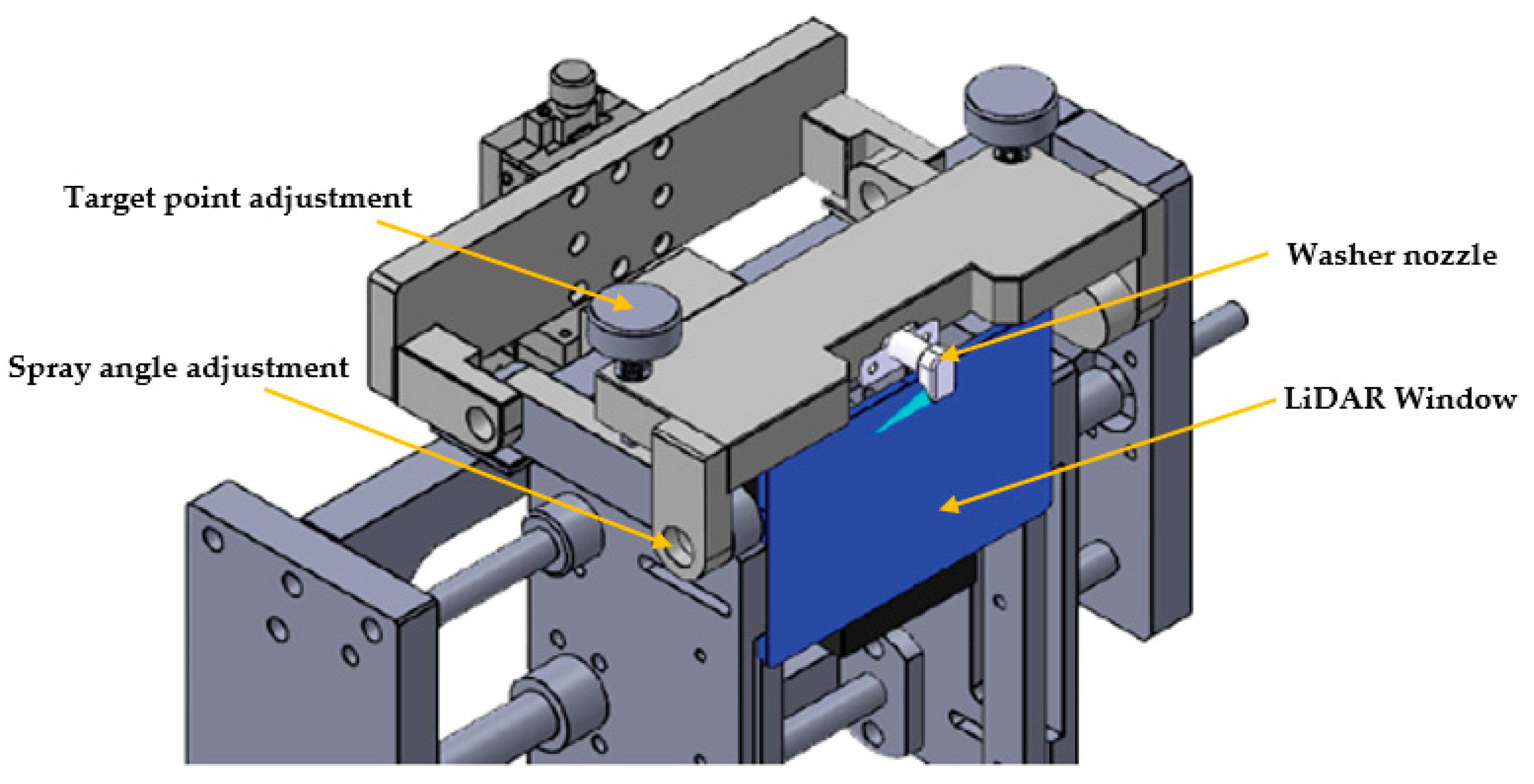
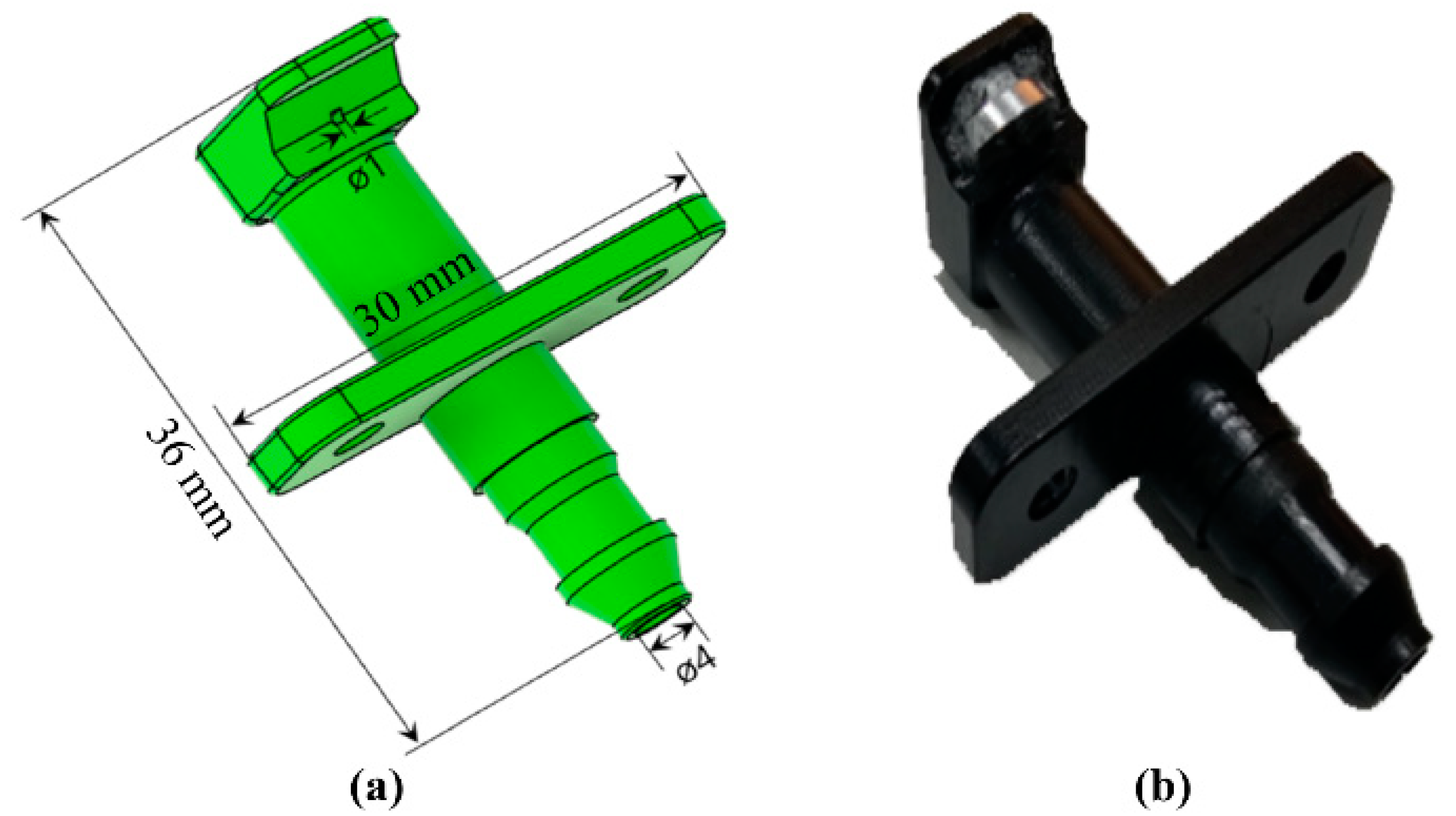
2.3.4. Washer Nozzle

A commonly used 60° fan-shaped spray-type nozzle was selected to reflect the representativeness of the washer nozzles. Further, 3D modeling was performed to produce the washer nozzle. A compact nozzle was designed for easy installation onto the test bench JIG and to ensure there was no interference to the FOV of the LiDAR. The geometry of the nozzle offered the benefit of easy spray angle and target point change, which were the considered variables in this study. Figure 8 shows the detailed 3D modeling design concept and prototype (manufacturer: SL corporation, Daegu, Republic of Korea) of the nozzle.

3. Results and Discussion

Figure A1 shows the photographs captured during the experiment. The cleaning area tendency for approximately four sprays could be identified for some of the 30 standards. The detailed experimental conditions are presented in Appendix A.1.
For the 30 standards selected for DOE, Table A2 shows the experiment results.

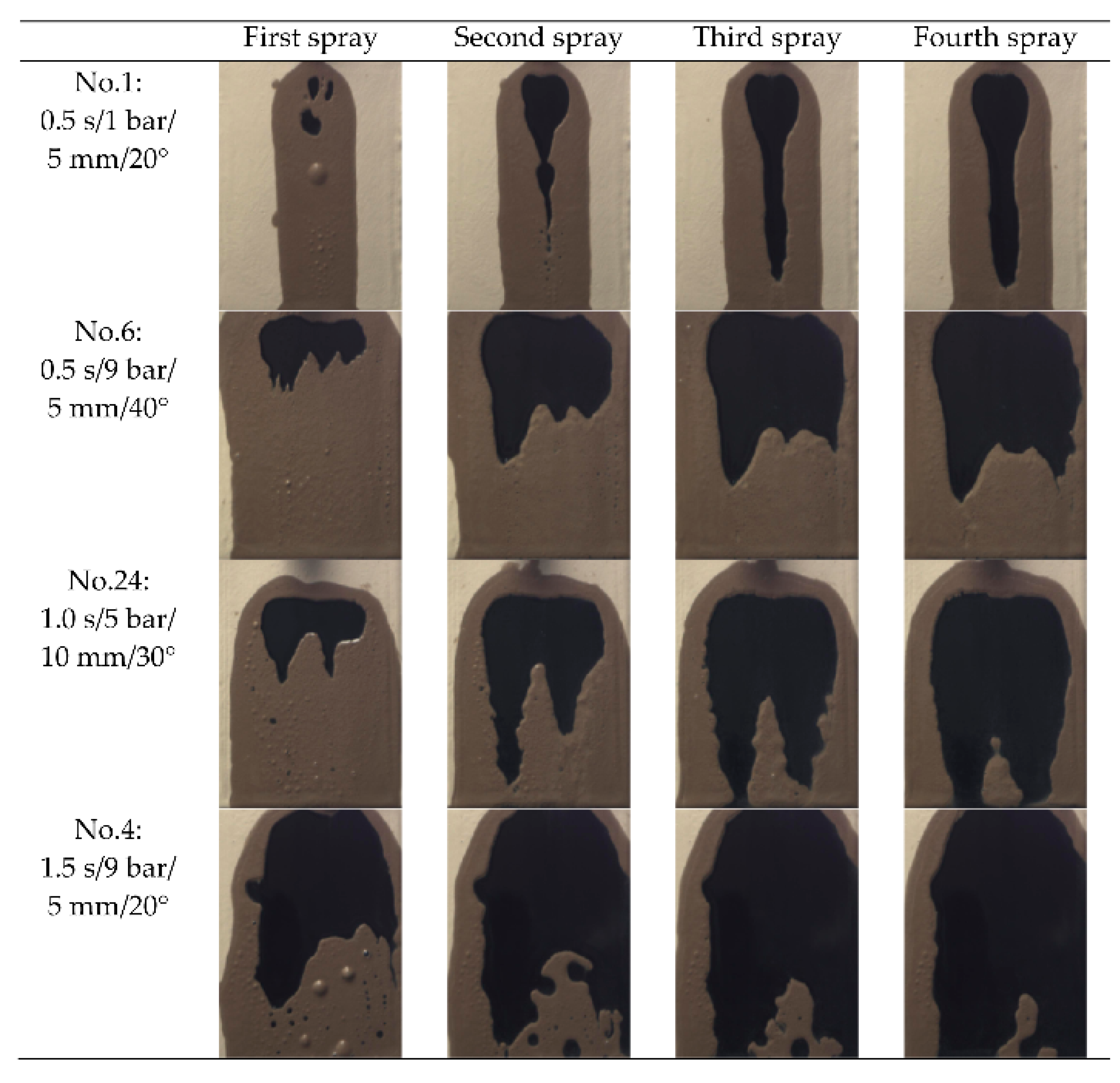
3.1. Optimized Cleaning Model for the Entire Target Area

As a result of analyzing the experimental data designed according to face-central composite design (FCCD) using the analysis of variance (ANOVA) technique for analysis of variance, a quadratic model was selected as the most suitable model. The statistics of the model according to the number of sprays are shown in Table 2. Adjusted (adj.) R-squared expressed the percentage at which the model expressed the data, whereas the F-value (p-value) denoted the statistical significance of the model. All quadratic model responses for the first to fourth sprays exhibited suitable and significant results. The model for the second spray showed the highest adjusted explanatory power (adj. R-squared) of 89%. If the R-squared value is explained by the entire model, the adj. R-squared value is the variable mean of squared regression obtained after considering the degrees of freedom divided by the mean of the square total.
Figure A2 shows that the residual normality verification results for all four models satisfied normality. Interactive terms were removed due to the absence of interactions between the factors. All models were found to be suitable because the lack of fit exceeded 0.05. The ANOVA results of the quadratic models based on the cleaning factor are presented in Table A3. The changes in cleaning rate by cleaning factors are shown in Figure A3.
For all four sprays, the primary terms of spray time and washer pressure were significant at a significance level of 5%. The quadratic term of the spray angle was significant at a significance level of 10% for the first spray, whereas the quadratic term of the washer pressure was significant at a significance level of 1% for the second to fourth sprays.
For the first spray, the cleaning rate increased with the spray time and washer pressure. The influence of the spray angle formed a curve. For the second spray, the cleaning rate increased with the spray time and washer pressure. However, unlike the first spray, the influence of the washer pressure formed a curve. The spray angle that influenced the curve formation for the first spray exhibited no difference in the cleaning rate. For the third spray, the same results as those of the second spray were observed, and the curve formed by the washer pressure was noticeable. The fourth spray exhibited similar tendencies, and the curve formed by the washer pressure was more noticeable. The spray angle and target point caused no change.

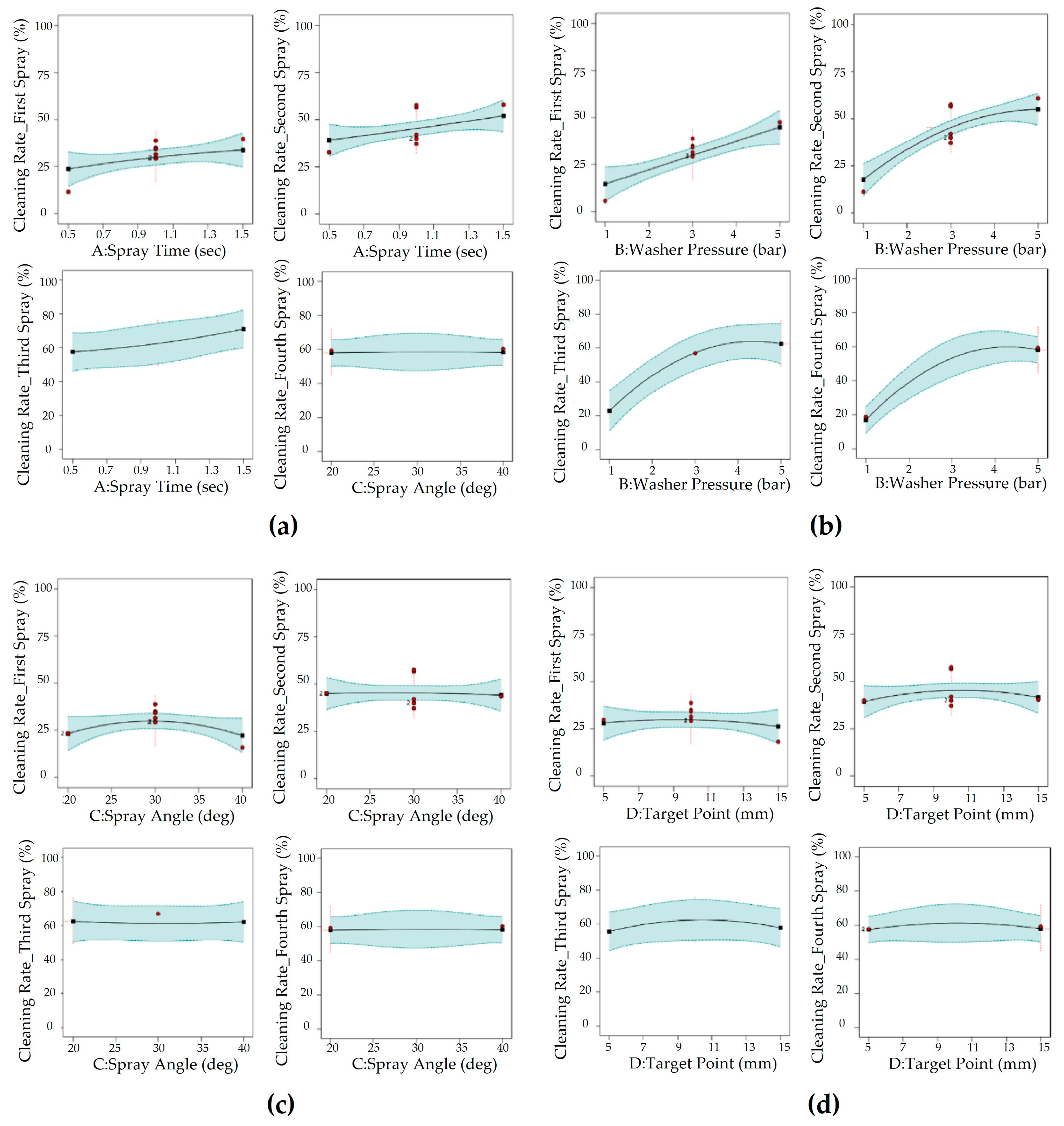
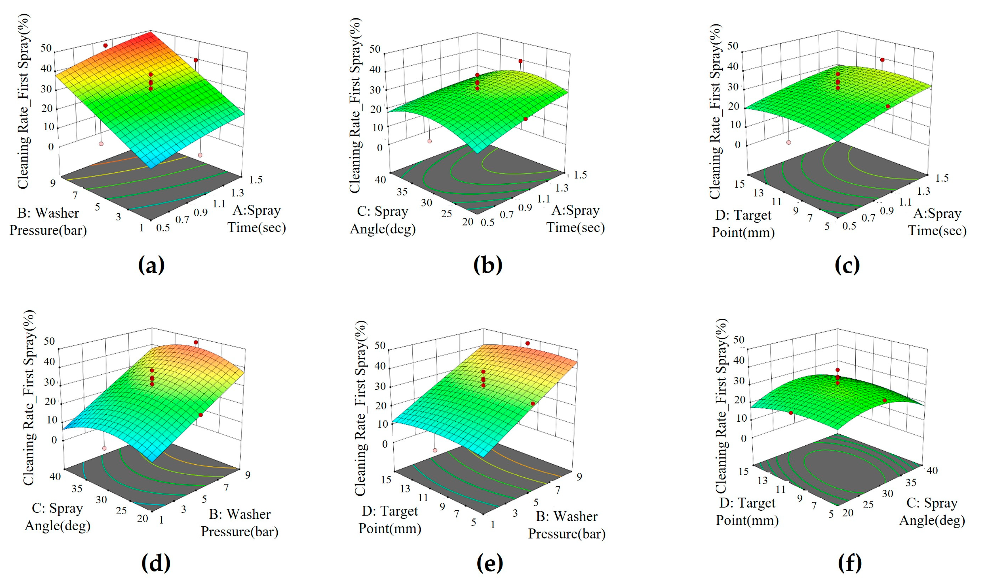
3.1.1. Results of the First Spray

To calculate the cleaning rate of the first spray, the quadratic model was most suitable as it showed high explanatory power with an R-squared value of 0.8666 and an adj. R-squared value of 0.8158. The adequate (adeq.) precision of the first spray model was 13.9004, exceeding the desired value of 4 and indicating its utility for navigating the design space. Variance analysis results of the first spray model are presented in Table 3.
In the first spray model, the primary terms of the spray time and washer pressure were significant at a significance level of 5%, and the quadratic term of the spray angle was significant at a significance level of 10%. When the regression coefficients of the factors were estimated based on the method of least squares, the quadratic equation was expressed as
Cleaning Rate (First spray) = −88.6166 + 10.0455 × spray time + 3.7811 × washer
pressure + 5.9701 × washer angle – 0.1003 × spray angle2
The 3D surface and 2D contour graphs drawn based on the quadratic equation of the first spray model are shown in Figure 9. The cleaning rate significantly increased with the washer pressure, and it showed a tendency to increase with the spray time. Initially, the cleaning rate increased with the spray angle, but it started to decrease as the angle continuously increased. Conversely, the cleaning rate barely changed or slightly decreased based on the target point.
As observed from the ANOVA results, the spray time and washer pressure had the largest impact on the cleaning rate, and the spray angle quadratically affected the cleaning rate.

3.1.2. Results of the Second Spray

To calculate the cleaning rate of the second spray, the quadratic model was most suitable, and it exhibited high explanatory power with an R-squared value of 0.9205 and adj. R-squared value of 0.8902. The adeq. Precision of the second spray model was 16.6642, which is considered appropriate as it exceeds 4. Variance analysis results of the second spray model are presented in Table 4.
In the second spray model, the primary terms of the spray time and washer pressure were significant at a significance level of 5%, and the quadratic term of the washer pressure was significant at a significance level of 5%. When the regression coefficients of the factors were estimated based on the method of least squares, the quadratic equation was expressed as
Cleaning Rate (Second spray) = −8.1076 + 12.9788 × spray time + 12.6699 ×
washer pressure – 0.7990 × washer pressure2
The 3D surface and 2D contour graphs drawn based on the quadratic equation of the second spray model are shown in Figure 10. The cleaning rate significantly increased with the washer pressure, and it tended to increase with the spray time. Initially, the cleaning rate increased alongside the target point, but it decreased as the target point further increased. Conversely, the cleaning rate barely changed with the increase in spray angle.
As observed from the ANOVA results, the washer pressure had the largest impact on the cleaning rate, and the cleaning rate increased according to the spray time. The washer pressure quadratically affected the cleaning rate.

3.1.3. Results of the Third Spray

To calculate the cleaning rate of the third spray, the quadratic model was most suitable, and it showed high explanatory power with an R-squared value of 0.9026 and adj. R-squared value of 0.8655. The adeq. Precision of the third spray model (14.173) was appropriate as it was higher than 4. Variance analysis results of the third spray model are presented in Table 5.
In the third spray model, the primary terms of the spray time and washer pressure were significant at a significance level of 5%, and the quadratic term of the washer pressure was significant at a significance level of 5%. When the regression coefficients of the factors were estimated based on the method of least squares, the quadratic equation was expressed as
Cleaning Rate (Third spray) = −4.0314 + 13.4966 × spray time + 15.3039 × washer
pressure – 1.0362 × washer pressure2
The 3D surface and 2D contour graphs drawn based on the quadratic equation of the third spray model are shown in Figure 11.
For the third spray model, tendencies similar to the results of the second spray model were observed, but the influence of the quadratic term of the washer pressure on the cleaning rate was larger. The cleaning rate significantly increased with the washer pressure, and it tended to increase with the spray time. Initially, the cleaning rate increased alongside the target point, but it decreased as the target point further increased. Conversely, the cleaning rate barely changed as the spray angle increased.

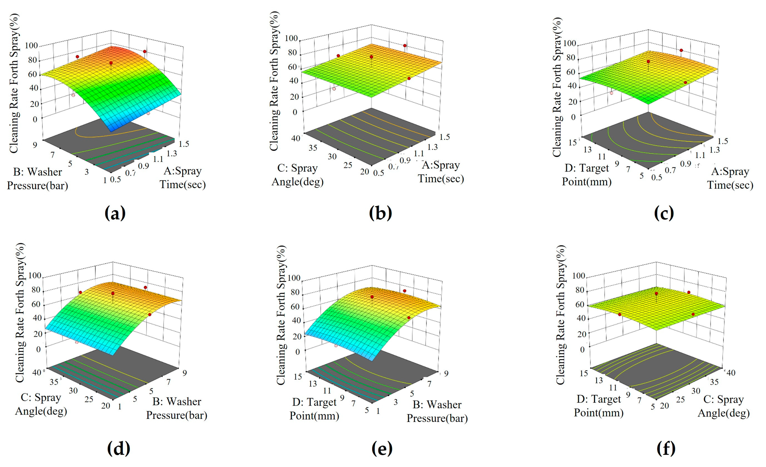
3.1.4. Results of the Fourth Spray

To calculate the cleaning rate of the fourth spray, the quadratic model was the most suitable and it showed high explanatory power with an R-squared value of 0.9147 and adj. R-squared value of 0.8822. The adeq. Precision of the fourth spray model (14.573) was appropriate as it was higher than 4. Variance analysis results of the fourth spray model are presented in Table 6.
In the fourth spray model, the primary terms of the spray time and washer pressure were significant at a significance level of 5%, and the quadratic term of the washer pressure was significant at a significance level of 5%. When the regression coefficients of the factors were estimated based on the method of least squares, the quadratic equation was expressed as
Cleaning Rate (Fourth spray) = −6.4554 + 13.9533 × spray time + 16.7453 ×
washer pressure – 1.1604 × washer pressure2
The 3D surface and 2D contour graphs drawn based on the quadratic equation of the fourth spray model are shown in Figure 12.
The results of the fourth spray model were similar to those of the third spray model. As observed from the ANOVA results, the washer pressure had the largest impact on the cleaning rate, and the cleaning rate increased according to the spray time. The washer pressure quadratically affected the cleaning rate.

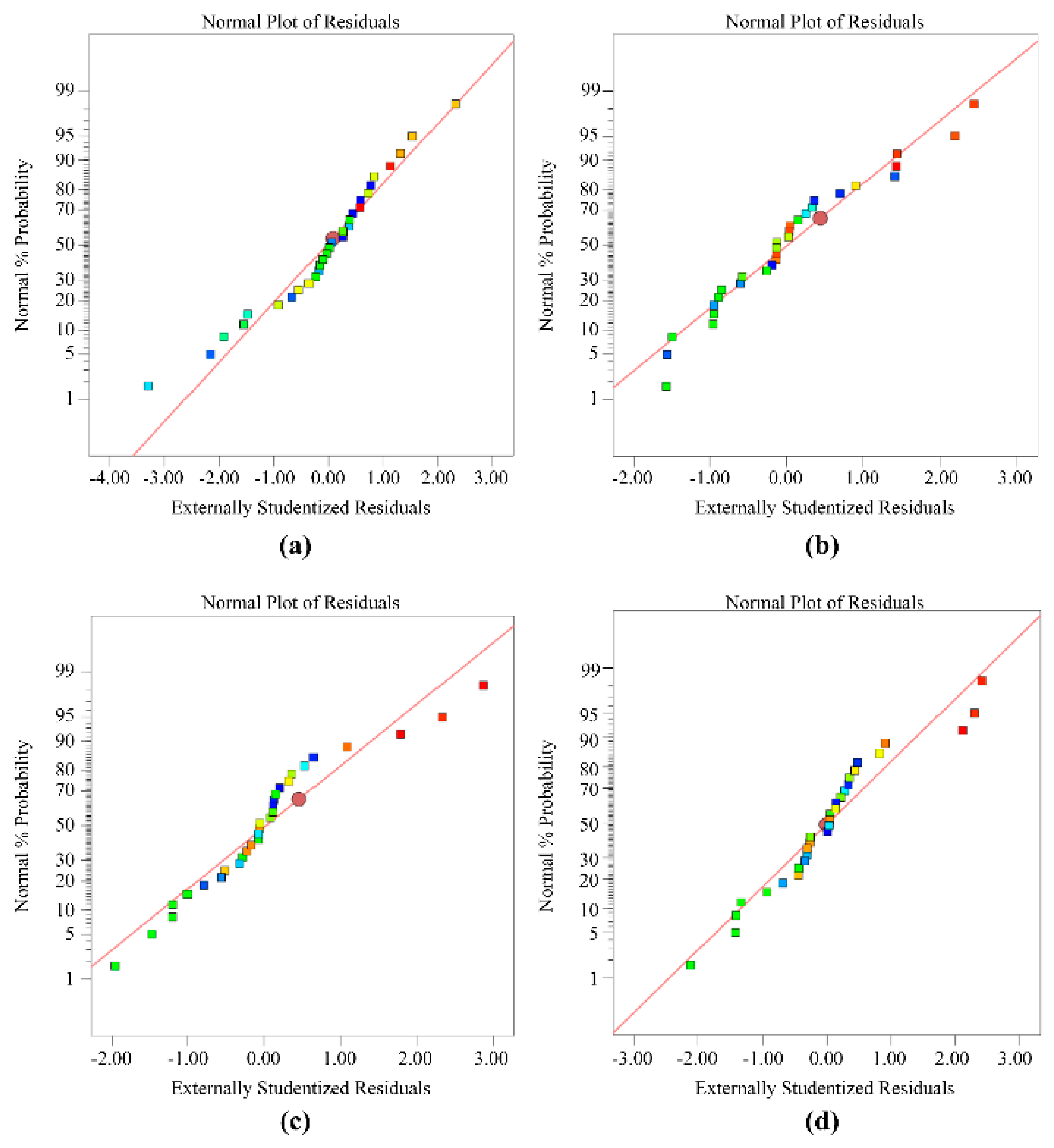
3.2. Optimization Results and Reproducibility Examination

As shown in Table 7, the optimal conditions of four factors were obtained based on the number of sprays for LiDAR cleaning. All four sprays met suitability, and the second spray showed the highest explanatory power. The target points were identical (10 mm), whereas the spray angles were approximately 30°, excluding that of the third spray. For the third and fourth sprays, the optimal conditions of time and pressure were similar, whereas the spray angle and cleaning rate were different. When experiments were performed under the calculated optimal conditions to examine reproducibility, the second spray model exhibited the smallest difference relative to the highest explanatory power of the model.
In this study, all cases were not tested by DOE. However, the optimized spray time and number of sprays were compared and the correlation between the two factors was obtained, as listed in Table 8. The cleaning rate was observed to increase with the spray time and number of sprays.
When the total spray time was 1 s, the cleaning rate was higher for two sprays at an interval of 0.5 s compared with one spray for 1 s. When the total spray time was 1.5 s, the cleaning rate was higher for three sprays at an interval of 0.5 s compared with one spray for 1.5 s. Thus, the cleaning rate was higher when the spray time was shorter and the spray was repeated under the same pressure and flow rate conditions, indicating the effectiveness of repeated sprays when compared with the spray time for a high cleaning rate.

4. Conclusions

This study investigated the effects of various factors, including washer pressure, spray time, spray angle, and target point, on the cleaning optimization direction of LiDAR sensors for autonomous driving technologies.
The results of this study suggest that washer pressure and spray time have the biggest impact on cleaning performance. However, the washer pressure cannot be infinitely increased due to physical limits and the cost of pumps. In this study, the effective water pressure was determined to be 7–8 bars based on the optimization results. Since spray time is related to the amount of water and more water is consumed with an increase in spray time, the washer reservoir tank capacity should be considered. Furthermore, the washer fluid obstructs the LiDAR sensor during spraying, and the resulting effect on sensor cleanliness may adversely affect the safety of autonomous driving operations. Accordingly, repeated spraying with short spray times (Table 8) was employed to ensure visibility even during washer operation. The highest cleaning rate was observed when the target point was positioned at approximately 10 mm. The optimal condition of the spray angle was observed to be between 20° and 30°.
A fan-shaped spray-type washer nozzle with a 60° spray angle, which is the most commonly used type of washer nozzle, was used in this study. In addition to the LiDAR window cover used in this study, various shapes can be created by adjusting the number of nozzles and applying them to window covers. The DOE was used to find the optimization direction while reducing a large number of experimentations, and the derived results were re-verified to secure the reliability of the optimization results. Detailed discussions on the experimental sample selection method, pretest, evaluation equipment, and analytical tools are expected to find applications to important materials selection by sensor cleaning-related manufacturers to develop technologies.

Author Contributions

Conceptualization, S.S.; methodology, S.S.; software, H.L; validation, H.-C.R.; formal analysis, J.J.; investigation, S.B. and H.C.; data curation, H.L.; writing—original draft preparation, S.S.; writing—review and editing, J.L. (Jungki Lee) and H.-C.R.; visualization, J.L. (Jangmin Lee) and W.L.; supervision, H.-C.R.; project administration, J.L. (Jungki Lee). All authors have read and agreed to the published version of the manuscript.

Funding

This work was supported by the Korea Agency for Infrastructure Technology Advancement (KAIA) grant funded by the Ministry of Land, Infrastructure and Transport (Project No. RS-2021_KA162419).

Institutional Review Board Statement

Not applicable.

Informed Consent Statement

Not applicable.

Data Availability Statement

The original contributions presented in the study are included in the article; further inquiries can be directed to the corresponding authors.

Acknowledgments

We thank Donghoon Bae of SL Company for their generous technical support of this study and Michael Lee for proofreading the statistics and manuscript.

Conflicts of Interest

Hongjun Cha and Seongguk Bae were employed by SL Co., Ltd. The remaining authors declare that the research was conducted in the absence of any commercial or financial relationships that could be construed as potential conflicts of interest.

Appendix A

Table A1. FCCD and four variables to optimize the cleaning rate.
No Coded Actual
X1X2X3X4X1X2X3X4Y
Spray TimeWasher PressureSpray AngleTarget PointSpray Time (s)Washer Pressure (bar)Spray
Angle (°)
Target
Point (mm)
Cleaning Rate (%)
1−1−1−1−10.5120516.42
2−11−1−10.5920557.83
31−1−1−11.5120532.01
411−1−11.5920581.38
5−1−11−10.5140519.54
6−111−10.5940555.21
71−11−11.5140526.56
8111−11.5940571.96
9−1−1−110.51201518.86
10−11−110.59201559.3
111−1−111.51201529.01
1211−111.59201570.41
13−1−1110.51401517.98
14−11110.59401560.38
151−1111.51401531.25
1611111.59401581.34
170−10011301025.88
18010019301073.33
19−10000.55301034.35
2010001.55301080.81
2100−1015201064.1
22001015401065.91
23000−11530564.35
24000115301556.55
25000015301051.6
26000015301078.3
27000015301056.81
28000015301057.01
29000015301056.33
30000015301054.71
Table A2. ANOVA results for cleaning factors.
Cleaning RateSourceSum of SquaresdfMean SquareF-Valuep-Value
First sprayA—Spray time454.111454.1111.570.0027 ***
B—Washer pressure4117.4814117.48104.91<0.0001 ***
C—Spray angle4.5314.530.11540.7374
D—Target point14.98114.980.38160.5434
A23.4813.480.08870.7688
B20.039810.03980.0010.9749
C2133.161133.163.390.0797 *
D218.66118.660.47550.498
Residual824.22139.25--
Lack of fit758.131647.383.590.082
Second sprayA—Spray time758.031758.0322.060.0001 ***
B—Washer pressure6305.6416305.64183.49<0.0001 ***
C—Spray angle3.2713.270.09510.7608
D—Target point22.6122.60.65770.4265
A20.17110.1710.0050.9444
B2207.911207.916.050.0227 **
C21.3511.350.03940.8445
D260.52160.521.760.1987
Residual721.652134.36--
Lack of fit311.121619.440.23680.9878
Third sprayA—Spray time819.721819.7216.060.0006 ***
B—Washer pressure7031.417031.4137.72<0.0001 ***
C—Spray angle0.435610.43560.00850.9273
D—Target point20.44120.440.40030.5338
A28.5418.540.16730.6867
B2546.211546.2110.70.0036 ***
C22.6512.650.05180.8221
D283.58183.581.640.2147
Residual1072.152151.05--
Lack of fit252.471615.780.09630.9999
Fourth sprayA—Spray time876.131876.1317.910.0004 ***
B—Washer pressure7611.3117611.31155.61<0.0001 ***
C—Spray angle0.330810.33080.00680.9352
D—Target point1110.02050.8875
A20.017510.01750.00040.9851
B2645.81645.813.20.0016 ***
C20.389710.38970.0080.9297
D232.52132.520.66490.424
Residual1027.152148.91--
Lack of fit266.571616.660.10950.9997
* p < 0.1, ** p < 0.05, *** p < 0.01.
Figure A1. Sample photographs of experimental results for four standards.
Applsci 14 08340 g0a1
Figure A2. Residual normality verification model for (a) first, (b) second, (c) third, and (d) fourth sprays.
Applsci 14 08340 g0a2
Figure A3. Changes in cleaning rate by cleaning factors with (a) spray time, (b) washer pressure, (c) spray angle, and (d) target point.
Applsci 14 08340 g0a3

Appendix A.1. Research Conditions and Methods

Appendix A.1.1. Blockage Conditions

For this study, the same test dust conditions were necessary to optimize the four variables of cleaning. First, as the area was fixed by the dust spray guide, the total amount of dust was fixed at 2.5 g. To identify the proper content of KL for ARI, the proportion of KL varied from 25 to 15, 5, and 2%, as listed in Table A3. Cleaning was performed at various washer pressures of 1, 3, 5, 7, and 9 bars. The test was aimed at examining the cleaning area results based on the pressure range and spray time because data at high (or low) performance were meaningless when cleaning was well (or not well) performed under low (or even high) performance conditions. In this study, the blockage produced by mixing ARI (48%), KL (2%), and water (50%) was sprayed onto the target LiDAR sensor to reproduce contamination of the sensor.
Table A3. Conformity experiment to select test blockage.
SymbolQuantityDescriptionAppropriateness
Arizona dust (ARI) 25%, Kaolin (KL) 25%, water 50%Applsci 14 08340 i001High viscosity, poor spraying conditionInappropriate
ARI 35%, KL 50%, water 50%Applsci 14 08340 i002
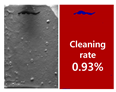
9 bar/s, low cleaning rate of the first sprayInappropriate
ARI 45%, KL 5%, water 50%Applsci 14 08340 i0031 bar/0.5 s, cleaning rate not confirmedInappropriate
ARI 48%, KL 2%, water 50%Applsci 14 08340 i0041 bar/0.5 s, cleaning rate confirmedAppropriate

Appendix A.1.2. Cleaning Conditions

Washer Pressure

The washer pressure was set as the main factor of design because the amount of water and target pressure increased with it. Considering that the pressure used in automobile washers ranged from 3 to 7 bars, a wider pressure range of 1 to 9 bars was considered in this study.

Spray Time

With an increase in washer spray time, the cleaning rate increased due to the increase in the absolute cleaning time. However, proper management was required because the time of blocking the LiDAR transmitter and receiver increased with the spray time. Therefore, the spray time was accordingly limited to a range of 0.5–1.5 s, and the drying time was limited to approximately 30 min without using a dryer for this study. Furthermore, the amount of washer fluid used is directly proportional to the spray duration. Previous studies have demonstrated that droplets on the sensor surface can significantly degrade LiDAR accuracy [17]. Hence, the presence of water droplets on the sensor surface during cleaning adversely affects the LiDAR performance.

Target Point

The target point was the first point of water injection and plays an important role in adjusting the cleaning area of the LiDAR. In this study, the target point was positioned in the range of 5 to 15 mm in the upward direction of the LiDAR window, considering that a wider range could increase the FOV interference and injection distance from the nozzle.

Spray Angle

The spray angle was the angle between the washer injection and LiDAR window surfaces used to determine the length of the nozzle protruding outside. The spray angle was limited to a range of 20°–40° because a wider range could interfere with the LiDAR FOV, similar to the target point.

Appendix A.1.3. Major Variables

The major variables are summarized in Table A4.
Table A4. Units of major variables.
TypeVariable
Manipulated variableWasher pressure, spray time, spray angle, target point
Control variableNozzle, spray distance, dust (ARI (48%): KL (2%): water (50%))
Dependent variableCleaning rate (%)

Appendix A.1.4. Purpose of DOE

DOE denotes planned design and analysis and represents a method of obtaining maximum information such as significant target analysis data from a minimum number of experiments to achieve the targeted goal. DOE included overall experimental design and analysis [18].
For DOE, response surface design was used to identify the effects of the selected factors on the response variable. The DOE method, shown in Figure A4, was mainly used to find factors that met process conditions or optimized the reaction value. The maximum or minimum points on the surface were found among all points on the plane or curved surface, and the line or surface that passed through the experiment results under optimal conditions was referred to as the response surface [19]. The data acquired according to the response surface design could identify the effects of several factors on the response variable (Y) and confirm the same through statistical analysis [20]. Therefore, in this study, the optimal point was found, and optimal conditions were derived by visually expressing the change in response value caused by the considered factors on a 3D surface. These processes were performed to predict the results according to the levels of influence offered by the factors and optimize the levels for LiDAR cleaning, which was the area of interest. After confirming the significance of the designed model, experiments were performed under optimal conditions and reproducibility was examined by comparing the expected response values with the experiment results. For response surface design, the number of experiments to be performed was determined by the number of influencing factors, the number of levels, and the functions of the response surface. The number of experiments and experimental methods were designed using the central composite design (CCD) or the Box–Behnken design method, which are most commonly used for response surface design [21,22].
Figure A4. DOE flow.
Applsci 14 08340 g0a4

Appendix A.1.5. Selection of DOE and Required Experimental Items

In this study, response surface methodology, specifically, face-centered central composite design (FCCD), was used to identify the optimal conditions for maximum cleaning rate. FCCD, where all axial points are projected onto the surfaces [23], was adopted for cleaning condition experiments, whereas the data analysis tool language R was used for response surface analysis. In the experimental design, the spray time, washer pressure, spray angle, and target point were encoded in three steps: −1, 0, and 1. The cleaning experiment was performed by setting conditions according to CCD, as shown in Table A5.
Table A5. Ranges and levels of four independent variables in the cleaning experiment.
VariableSymbolRange of Levels
Low (−1)Centre (0)High (1)
Spray time (s)X10.511.5
Washer pressure (bar)X2159
Spray angle (°)X3203040
Target point (mm)X451015

Appendix A.1.6. Results Analysis Method

The results analysis aimed to calculate the area with the same standards. To analyze 30 samples under the same standards, original images were captured using an image analysis software program(ver.2023), and photographs were obtained after each spray. As shown in Figure A5, the dust (red) and LiDAR cover (blue) colors were distinguished, promoting automatic calculation of the cleaning area.
Figure A5. Example of area calculation: (a) Actual photograph before and (b) after area analysis.
Applsci 14 08340 g0a5

References

  1. Kenk, M.A.; Hassaballah, M. Vehicle detection in adverse weather nature dataset. arXiv 2020, arXiv:2008.05402v1. [Google Scholar] [CrossRef]
  2. Qian, R.; Tan, R.T.; Yang, W.; Su, J.; Liu, J. Attentive generative adversarial network for raindrop removal from a single image. In Proceedings of the 2018 IEEE/CVF Conference on Computer Vision and Pattern Recognition, Salt Lake City, UT, USA, 18–23 June 2018; pp. 2482–2491. [Google Scholar] [CrossRef]
  3. Porav, H.; Bruls, T.; Newman, P. I can see clearly now: Image restoration via de-raining. In Proceedings of the 2019 International Conference on Robotics and Automation (ICRA), Montreal, QC, Canada, 20–24 May 2019; pp. 7087–7093. [Google Scholar] [CrossRef]
  4. Agunbiade, Y.O.; Dehinbo, J.O.; Zuva, T.; Akanbi, A.K. Road detection technique using filters with application to autonomous driving system. arXiv 2018, arXiv:1809.05878v1. [Google Scholar] [CrossRef]
  5. Son, S.; Lee, W.; Jung, H.; Lee, J.; Kim, C.; Lee, H.; Park, H.; Lee, H.; Jang, J.; Cho, S.; et al. Evaluation of camera recognition performance under blockage using virtual test drive toolchain. Sensors 2023, 23, 8027. [Google Scholar] [CrossRef] [PubMed]
  6. The Korea Times. Hyundai Motor Group Develops Camera Sensor Cleaning System. September 2023. Available online: https://www.koreatimes.co.kr/www/tech/2023/09/129_358624.html (accessed on 6 September 2023).
  7. Xenomatix. Sensor Cleaning. February 2022. Available online: https://xenomatix.com/sensor-cleaning (accessed on 11 February 2022).
  8. 2023 BMW 7 Series: Keeping It Clean with Front and Rear Sensor Cleaning. BMW of Schererville YouTube. March 2023. Available online: https://youtube.com/shorts/W95GHJGUfJw?si=X0Cmd7S0f8e8oaUB (accessed on 30 March 2023).
  9. Cleaning Mercedes Sensor. Sensor Guides. January 2024. Available online: https://sensorguides.com/are-dirty-sensors-impacting-your-mercedes-discover-the-ultimate-cleaning-techniques/ (accessed on 20 January 2024).
  10. Das, A. SolidNet: Soiling degradation detection in autonomous driving. arXiv 2019, arXiv:1911.01054v2. [Google Scholar] [CrossRef]
  11. Sheeny, M.; De Pellegrin, E.; Mukherjee, S.; Ahrabian, A.; Wang, S.; Wallace, A. RADIATE: A radar dataset for automotive perception in bad weather. In Proceedings of the 2021 IEEE International Conference on Robotics and Automation (ICRA), Xi’an, China, 30 May–5 June 2021; pp. 1–7. [Google Scholar] [CrossRef]
  12. Göktürk, K.; Jönsson, A. Developing a Resource-Efficient Sensor Cleaning System for Autonomous Heavy Vehicles. Master’s Thesis, KTH, Stockholm, Sweden, 2019. [Google Scholar]
  13. Son, S.; Lee, W.; Jung, H.; Lee, J.; Kim, C.; Lee, H.; Cho, S.; Jang, J.; Lee, M.; Ryu, H.-C. Experimental analysis of various blockage performance for LiDAR sensor cleaning evaluation. Sensors 2023, 23, 2752. [Google Scholar] [CrossRef] [PubMed]
  14. Shah, S.; Pattankar, R.; Varghese, R.; Pai, B.H.A.; Yenugu, S.; Wolbeck, A.; Balluff, S.; Schmid, H.; Duggirala, R. Digital Methodology for Simulating Autonomous Vehicle Sensor Cleaning. SAE Mobilus Technical Paper 2024-26-0006. SAE International: Warrendale, PA, USA, 2024. [CrossRef]
  15. Gomes, T.; Roriz, R.; Cunha, L.; Ganal, A.; Soares, N.; Araújo, T.; Monteiro, J. Evaluation and testing system for automotive LiDAR sensors. Appl. Sci. 2022, 12, 13003. [Google Scholar] [CrossRef]
  16. Kral, W.; Dalpez, S. Modular sensor cleaning system for autonomous driving. ATZ Worldw. 2018, 120, 56–59. [Google Scholar] [CrossRef]
  17. Pao, W.Y.; Howorth, J.; Li, L.; Agelin-Chaab, M.; Roy, L.; Knutzen, J.; Baltazar-y-Jimenez, A.; Muenker, K. Investigation of automotive LiDAR vision in rain from material and optical perspectives. Sensors 2024, 24, 2997. [Google Scholar] [CrossRef] [PubMed]
  18. Durakovic, B. Design of experiments application, concepts, examples: State of the art. Periodicals Eng. Nat. Sci. 2017, 5. [Google Scholar] [CrossRef]
  19. Geiger, E.O. Statistical methods for fermentation optimization. In Fermentation and Biochemical Engineering Handbook, 3rd ed.; Vogel, H.C., Todaro, C.M., Eds.; William Andrew Publishing: Norwich, NY, USA, 2014; pp. 415–422. [Google Scholar] [CrossRef]
  20. Khuri, A.I.; Mukhopadhyay, S. Response surface methodology. WIREs Comput. Stats. 2010, 2, 128–149. [Google Scholar] [CrossRef]
  21. Rosales, E.; Sanromán, M.A.; Pazos, M. Application of central composite face-centered design and response surface methodology for the optimization of electro-Fenton decolorization of Azure B dye. Environ. Sci. Pollut. Res. Int. 2012, 19, 1738–1746. [Google Scholar] [CrossRef] [PubMed]
  22. Ranade, S.S.; Thiagarajan, P. Selection of a design for response surface. IOP Conf. Ser.: Mater. Sci. Eng. 2017, 263, 022043. [Google Scholar] [CrossRef]
  23. Balachandran, M.; Devanathan, S.; Muraleekrishnan, R.; Bhagawan, S.S. Optimizing properties of nanoclay–nitrile rubber (NBR) composites using face centred central composite design. Mater. Des. 2012, 35, 854–862. [Google Scholar] [CrossRef]
Figure 1. Sensor’s washer fixing equipment.
Applsci 14 08340 g001
Figure 2. Blockage cleaning test bench: (a) overall and (b) inside views.
Applsci 14 08340 g002
Figure 3. Blockage performance graphs: (a) Basic dust and (b) KL additive performance results. ARI = Arizona dust, JIS = Japanese Industrial Standards, KTD = Korean test dust, KL = Kaolin, FP = fake poop [13].
Applsci 14 08340 g003
Figure 4. Actual G32 LiDAR (AutoL).
Applsci 14 08340 g004
Figure 5. G32 LiDAR window cover specification.
Applsci 14 08340 g005
Figure 6. G32 LiDAR transceiver main area (A zone: transmitter; B zone: receiver).
Applsci 14 08340 g006
Figure 7. Dust spray guide production: (a) Design draft and (b) actual prototype.
Applsci 14 08340 g007
Figure 8. Test nozzle: (a) Design draft and (b) actual prototype.
Applsci 14 08340 g008
Figure 9. Three-dimensional graphs of the cleaning rate of the first spray to (a) washer pressure and spray time, (b) spray angle and spray time, (c) target point and spray time, (d) spray angle and washer pressure, (e) target point and washer pressure, and (f) target point and spray angle.
Applsci 14 08340 g009
Figure 10. Three-dimensional graphs of the cleaning rate of the second spray to (a) washer pressure and spray time, (b) spray angle and spray time, (c) target point and spray time, (d) spray angle and washer pressure, (e) target point and washer pressure, and (f) target point and spray angle.
Applsci 14 08340 g010
Figure 11. Three-dimensional graphs of the cleaning rate of the third spray to (a) washer pressure and spray time, (b) spray angle and spray time, (c) target point and spray time, (d) spray angle and washer pressure, (e) target point and washer pressure, and (f) target point and spray angle.
Applsci 14 08340 g011
Figure 12. Three-dimensional graphs of the cleaning rate of the fourth spray to (a) washer pressure and spray time, (b) spray angle and spray time, (c) target point and spray time, (d) spray angle and washer pressure, (e) target point and washer pressure, and (f) target point and spray angle.
Applsci 14 08340 g012
Table 1. G32 LiDAR specifications.
TypeSpecifications
SensorNumber of channels: 32
Range: 300 m (@80%), 100 m (@10%)Horizontal field of view: 135°
Horizontal angular resolution: 0.117°
Vertical field of view: 10°
Vertical angular resolution: 0.3125°
Range resolution: 4 mm
Range accuracy: Up to 30 mm
LaserFrame rate: 25 fps
Wavelength: 905 nm
DeviceSize 128 × 76 × 96 mm
Table 2. ANOVA results for quadratic models with varying cleaning rates.
Model
Response
R-SquaredAdj.
R-Squared
Adeq.
Precision
F-Valuep-Value
First spray0.86660.815813.900417.06<0.0001 **
Second spray0.92050.890216.664230.39<0.0001 **
Third spray0.90260.865514.17324.33<0.0001 **
Fourth spray0.91470.882214.57328.16<0.0001 **
** p < 0.05.
Table 3. Variance analysis results of the first spray model.
Model
Response
R-SquaredAdj.
R-Squared
Adeq.
Precision
F-Valuep-Value
First spray0.86660.815813.900417.06<0.0001 **
** p < 0.05.
Table 4. Variance analysis results of the second spray model.
Model
Response
R-SquaredAdj.
R-Squared
Adeq.
Precision
F-Valuep-Value
Second spray0.92050.890216.664230.39<0.0001 **
** p < 0.05.
Table 5. Variance analysis results of the third spray model.
Model
Response
R-SquaredAdj.
R-Squared
Adeq.
Precision
F-Valuep-Value
Third spray0.92060.865514.17324.33<0.0001 **
** p < 0.05.
Table 6. Variance analysis results of the fourth spray model.
Model
Response
R-SquaredAdj.
R-Squared
Adeq.
Precision
F-Valuep-Value
Fourth spray0.91470.882214.57328.16<0.0001 **
** p < 0.05.
Table 7. Optimization factors according to the number of sprays.
Optimal Factor1st Spray Model2nd Spray Model3rd Spray Model4th Spray Model
Spray time1.412751.464061.51.5
Spray angle27.245623.806520.000231.7463
Washer pressure8.935888.1816777.724577.60159
Target point8.133811.598810.479610.1625
Adj. R-squared0.81580.89020.86550.8822
Predicted cleaning rate47.539861.065572.596377.7102
Actual cleaning rate39.3462.970.3174.69
Diff (predicted-actual)8.201.8345−2.2863−3.0202
Table 8. Comparison of cleaning rates according to spray time and number of sprays.
Spray
Time (s)
1st Spray
Result (%)
2nd Spray
Result (%)
3rd Spray
Result (%)
4th Spray
Result (%)
0.538.3707248.5530759.0996363.75687
1.043.393555.0425265.8479770.73354
1.548.4162861.5319672.596377.7102
Disclaimer/Publisher’s Note: The statements, opinions and data contained in all publications are solely those of the individual author(s) and contributor(s) and not of MDPI and/or the editor(s). MDPI and/or the editor(s) disclaim responsibility for any injury to people or property resulting from any ideas, methods, instructions or products referred to in the content.

