Figure 1.
Design case 1 fed by 9 CORPSs blocks of 4 inputs and 9 outputs.
Figure 1.
Design case 1 fed by 9 CORPSs blocks of 4 inputs and 9 outputs.
Figure 2.
Phase plane generated by the design or 2-D phased array system 1.
Figure 2.
Phase plane generated by the design or 2-D phased array system 1.
Figure 3.
Design case 2 using two stages of CORPSs blocks of 4 inputs and 9 outputs.
Figure 3.
Design case 2 using two stages of CORPSs blocks of 4 inputs and 9 outputs.
Figure 4.
Phase plane generated by the design or 2-D phased array system 2.
Figure 4.
Phase plane generated by the design or 2-D phased array system 2.
Figure 5.
CORPSs feeding system of 4 inputs and 9 outputs, including the dimension values.
Figure 5.
CORPSs feeding system of 4 inputs and 9 outputs, including the dimension values.
Figure 6.
Behavior of the (a) reflection coefficients and the (b) match impedance of the feeding system.
Figure 6.
Behavior of the (a) reflection coefficients and the (b) match impedance of the feeding system.
Figure 7.
Behavior of the transmission coefficients of the novel 4 × 9 feeding system.
Figure 7.
Behavior of the transmission coefficients of the novel 4 × 9 feeding system.
Figure 8.
Crossover design of the novel 4 × 9 feeding system: (a) top view, (b) manufactured prototype, (c) rear view, and (d) reflection and transmission coefficients.
Figure 8.
Crossover design of the novel 4 × 9 feeding system: (a) top view, (b) manufactured prototype, (c) rear view, and (d) reflection and transmission coefficients.
Figure 9.
Division or combination node (ring type): (a) prototype and (b) design in CST with dimensions.
Figure 9.
Division or combination node (ring type): (a) prototype and (b) design in CST with dimensions.
Figure 10.
Behavior of the transmission and reflection coefficients for the ring-type node: (a) simulated and (b) measurements.
Figure 10.
Behavior of the transmission and reflection coefficients for the ring-type node: (a) simulated and (b) measurements.
Figure 11.
Behavior of the phase through the 4 × 9 CORPSs feeding system.
Figure 11.
Behavior of the phase through the 4 × 9 CORPSs feeding system.
Figure 12.
Antenna element selected to assess the 2-D phased array systems: (a) CST design and (b) prototype.
Figure 12.
Antenna element selected to assess the 2-D phased array systems: (a) CST design and (b) prototype.
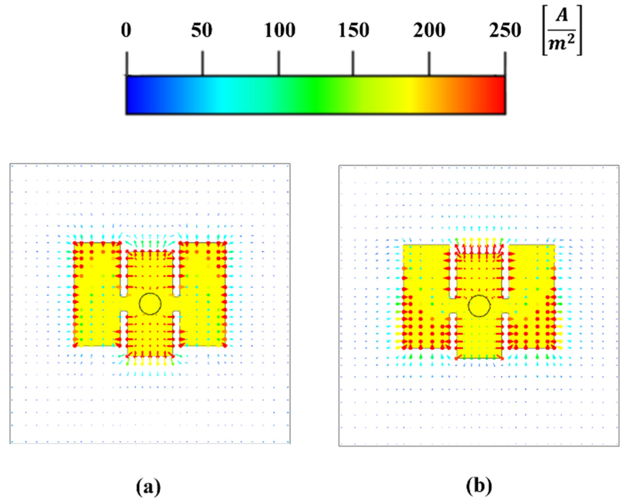
Figure 13.
Current distribution of the chosen element for (a) 5.75 GHz and (b) 6.0 GHz.
Figure 13.
Current distribution of the chosen element for (a) 5.75 GHz and (b) 6.0 GHz.
Figure 14.
Behavior of the reflection coefficient of the chosen antenna element.
Figure 14.
Behavior of the reflection coefficient of the chosen antenna element.
Figure 15.
Radiation pattern of the chosen element obtained by the simulation (blue color) in CST and experimental measurements (red color): (a) 5.5 GHz, (b) 5.75 GHz, (c) 6.0 GHz and (d) 5.75 GHz (cut at the azimuth plane).
Figure 15.
Radiation pattern of the chosen element obtained by the simulation (blue color) in CST and experimental measurements (red color): (a) 5.5 GHz, (b) 5.75 GHz, (c) 6.0 GHz and (d) 5.75 GHz (cut at the azimuth plane).
Figure 16.
Active reflection coefficient for the cases of the worst and best performance of the two proposed 2-D architectures.
Figure 16.
Active reflection coefficient for the cases of the worst and best performance of the two proposed 2-D architectures.
Figure 17.
Two-dimensional phased array and 3-D radiation pattern for the proposed systems, case 2: (a) ϕ0 = 15° and θ0 = 18°, (b) ϕ0 = 30° and θ0 = 10°, case 1: (c) ϕ0 = 20° and θ0 = 10° and (d) ϕ0 = 40° and θ0 = 18°.
Figure 17.
Two-dimensional phased array and 3-D radiation pattern for the proposed systems, case 2: (a) ϕ0 = 15° and θ0 = 18°, (b) ϕ0 = 30° and θ0 = 10°, case 1: (c) ϕ0 = 20° and θ0 = 10° and (d) ϕ0 = 40° and θ0 = 18°.
Figure 18.
Worst case of the losses in gain of the proposed antenna system, considering beam-scanning.
Figure 18.
Worst case of the losses in gain of the proposed antenna system, considering beam-scanning.
Figure 19.
Behavior of the radiation pattern at 5.5 GHz, 5.75 GHz and 6.0 GHz for θ0 = 18°.
Figure 19.
Behavior of the radiation pattern at 5.5 GHz, 5.75 GHz and 6.0 GHz for θ0 = 18°.
Figure 20.
Behavior of the radiation pattern at the farthest scanning angle of θ0 = 30° and ϕ0 = 0°.
Figure 20.
Behavior of the radiation pattern at the farthest scanning angle of θ0 = 30° and ϕ0 = 0°.
Figure 21.
Behavior of the mutual coupling between different antenna elements (1, 11, 21, 31, 40, 41) that include different spacing between them.
Figure 21.
Behavior of the mutual coupling between different antenna elements (1, 11, 21, 31, 40, 41) that include different spacing between them.
Table 1.
Phase values at the input ports of the feeding system for (θ0 = 10° and ϕ0 = 0°) (Conf. 2).
Table 1.
Phase values at the input ports of the feeding system for (θ0 = 10° and ϕ0 = 0°) (Conf. 2).
| Block | | | | |
|---|
| 1 | 0 | −187.54 | −62.51 | −250.05 |
| 2 | 0 | −187.54 | −62.51 | −250.05 |
| 3 | 0 | −187.54 | −62.51 | −250.05 |
| 4 | 0 | −187.54 | −62.51 | −250.05 |
Table 2.
Phase values at the output ports of the feeding system for (θ0 = 10° and ϕ0 = 0°) (Conf. 2).
Table 2.
Phase values at the output ports of the feeding system for (θ0 = 10° and ϕ0 = 0°) (Conf. 2).
| Block | | | | | | | | | |
|---|
| 5 | 0 | −31.25 | −62.51 | −93.77 | −125.02 | −156.28 | −187.54 | −218.79 | −250.05 |
| 6 | 0 | −31.25 | −62.51 | −93.77 | −125.02 | −156.28 | −187.54 | −218.79 | −250.05 |
| 7 | 0 | −31.25 | −62.51 | −93.77 | −125.02 | −156.28 | −187.54 | −218.79 | −250.05 |
| 8 | 0 | −31.25 | −62.51 | −93.77 | −125.02 | −156.28 | −187.54 | −218.79 | −250.05 |
| 9 | 0 | −31.25 | −62.51 | −93.77 | −125.02 | −156.28 | −187.54 | −218.79 | −250.05 |
| 10 | 0 | −31.25 | −62.51 | −93.77 | −125.02 | −156.28 | −187.54 | −218.79 | −250.05 |
| 11 | 0 | −31.25 | −62.51 | −93.77 | −125.02 | −156.28 | −187.54 | −218.79 | −250.05 |
| 12 | 0 | −31.25 | −62.51 | −93.77 | −125.02 | −156.28 | −187.54 | −218.79 | −250.05 |
| 13 | 0 | −31.25 | −62.51 | −93.77 | −125.02 | −156.28 | −187.54 | −218.79 | −250.05 |
Table 3.
Phase values at the input ports of the feeding system for (θ0 = 15° and ϕ0 = 10°) (Conf. 2).
Table 3.
Phase values at the input ports of the feeding system for (θ0 = 15° and ϕ0 = 10°) (Conf. 2).
| Block | | | | |
|---|
| 1 | 0 | −275.27 | −91.75 | −367.03 |
| 2 | −16.17 | −291.45 | −107.93 | −383.21 |
| 3 | −48.53 | −323.81 | −140.29 | −156.47 |
| 4 | −64.71 | −339.99 | −156.47 | −431.75 |
Table 4.
Phase values at the output ports of the feeding system for (θ0 = 15° and ϕ0 = 10°) (Conf. 2).
Table 4.
Phase values at the output ports of the feeding system for (θ0 = 15° and ϕ0 = 10°) (Conf. 2).
| Block | | | | | | | | | |
|---|
| 5 | 0 | −45.88 | −91.76 | −137.64 | −183.52 | −229.40 | −275.28 | −321.16 | −367.04 |
| 6 | −8.09 | −53.97 | −99.85 | −145.73 | −191.61 | −237.49 | −283.37 | −329.25 | −375.13 |
| 7 | −16.18 | −62.06 | −107.94 | −153.82 | −199.70 | −245.58 | −291.46 | −337.34 | −383.22 |
| 8 | −24.27 | −70.15 | −116.03 | −161.91 | −207.79 | −253.67 | −299.55 | −345.43 | −391.31 |
| 9 | −32.36 | −78.24 | −124.12 | −170.00 | −215.88 | −261.76 | −307.64 | −353.52 | −399.40 |
| 10 | −40.45 | −86.33 | −132.21 | −178.09 | −223.97 | −269.85 | −315.73 | −361.61 | −407.49 |
| 11 | −48.54 | −94.42 | −140.30 | −186.18 | −232.06 | −277.94 | −323.82 | −369.70 | −415.58 |
| −56.63 | −102.51 | −148.39 | −194.27 | −240.15 | −286.03 | −331.91 | −377.79 | −423.67 |
| 13 | −64.72 | −110.60 | −156.48 | −202.36 | −248.24 | −294.12 | −340.00 | −385.88 | −431.76 |
Table 5.
Phase values at the input ports of the feeding system for (θ0 = 5° and ϕ0 = 0°) (Conf. 1).
Table 5.
Phase values at the input ports of the feeding system for (θ0 = 5° and ϕ0 = 0°) (Conf. 1).
| Block | | | | |
|---|
| 1 | 0.00 | −31.38 | −94.13 | −125.50 |
| 2 | 0.00 | −31.38 | −94.13 | −125.50 |
| 3 | 0.00 | −31.38 | −94.13 | −125.50 |
| 4 | 0.00 | −31.38 | −94.13 | −125.50 |
| 5 | 0.00 | −31.38 | −94.13 | −125.50 |
| 6 | 0.00 | −31.38 | −94.13 | −125.50 |
| 7 | 0.00 | −31.38 | −94.13 | −125.50 |
| 8 | 0.00 | −31.38 | −94.13 | −125.50 |
| 9 | 0.00 | −31.38 | −94.13 | −125.50 |
Table 6.
Phase values at the output ports of the feeding system for (θ0 = 5° and ϕ0 = 0°) (Conf. 1).
Table 6.
Phase values at the output ports of the feeding system for (θ0 = 5° and ϕ0 = 0°) (Conf. 1).
| Block | | | | | | | | | |
|---|
| 1 | 0.00 | −15.69 | −31.38 | −47.06 | −62.75 | −78.44 | −94.13 | −109.82 | −125.50 |
| 2 | 0.00 | −15.69 | −31.38 | −47.06 | −62.75 | −78.44 | −94.13 | −109.82 | −125.50 |
| 3 | 0.00 | −15.69 | −31.38 | −47.06 | −62.75 | −78.44 | −94.13 | −109.82 | −125.50 |
| 4 | 0.00 | −15.69 | −31.38 | −47.06 | −62.75 | −78.44 | −94.13 | −109.82 | −125.50 |
| 5 | 0.00 | −15.69 | −31.38 | −47.06 | −62.75 | −78.44 | −94.13 | −109.82 | −125.50 |
| 6 | 0.00 | −15.69 | −31.38 | −47.06 | −62.75 | −78.44 | −94.13 | −109.82 | −125.50 |
| 7 | 0.00 | −15.69 | −31.38 | −47.06 | −62.75 | −78.44 | −94.13 | −109.82 | −125.50 |
| 8 | 0.00 | −15.69 | −31.38 | −47.06 | −62.75 | −78.44 | −94.13 | −109.82 | −125.50 |
| 9 | 0.00 | −15.69 | −31.38 | −47.06 | −62.75 | −78.44 | −94.13 | −109.82 | −125.50 |
Table 7.
Phase values at the input ports of the feeding system for (θ0 = 10° and ϕ0 = 15°) (Conf. 1).
Table 7.
Phase values at the input ports of the feeding system for (θ0 = 10° and ϕ0 = 15°) (Conf. 1).
| Block | | | | |
|---|
| 1 | 0.00 | −60.38 | −181.15 | −241.53 |
| 2 | −8.09 | −68.47 | −189.24 | −249.62 |
| 3 | −16.18 | −76.56 | −197.33 | −257.71 |
| 4 | −24.27 | −84.65 | −205.42 | −265.80 |
| 5 | −32.36 | −92.74 | −213.51 | −273.89 |
| 6 | −40.45 | −100.83 | −221.60 | −281.98 |
| 7 | −48.54 | −108.92 | −229.69 | −290.07 |
| 8 | −56.63 | −117.01 | −237.78 | −298.16 |
| 9 | −64.72 | −125.10 | −245.87 | −306.25 |
Table 8.
Phase values at the output ports of the feeding system for (θ0 = 10° and ϕ0 = 15°) (Conf. 1).
Table 8.
Phase values at the output ports of the feeding system for (θ0 = 10° and ϕ0 = 15°) (Conf. 1).
| Block | | | | | | | | | |
|---|
| 1 | 0.00 | −30.19 | −60.38 | −90.57 | −120.77 | −150.96 | −181.15 | −211.34 | −241.53 |
| 2 | −8.09 | −38.28 | −68.47 | −98.66 | −128.86 | −159.05 | −189.24 | −219.43 | −249.62 |
| 3 | −16.18 | −46.37 | −76.56 | −106.75 | −136.95 | −167.14 | −197.33 | −227.52 | −257.71 |
| 4 | −24.27 | −54.46 | −84.65 | −114.84 | −145.04 | −175.23 | −205.42 | −235.61 | −265.80 |
| 5 | −32.36 | −62.55 | −92.74 | −122.93 | −153.13 | −183.32 | −213.51 | −243.70 | −273.89 |
| 6 | −40.45 | −70.64 | −100.83 | −131.02 | −161.22 | −191.41 | −221.60 | −251.79 | −281.98 |
| 7 | −48.54 | −78.73 | −108.92 | −139.11 | −169.31 | −199.50 | −229.69 | −259.88 | −290.07 |
| 8 | −56.63 | −86.82 | −117.01 | −147.20 | −177.40 | −207.59 | −237.78 | −267.97 | −298.16 |
| 9 | −64.72 | −94.91 | −125.10 | −155.29 | −185.49 | −215.68 | −245.87 | −276.06 | −306.25 |
Table 9.
Amplification values (at the outputs of the feeding system) that are required to obtain a raised cosine for θ0 = 30° and ϕ0 = 0° (Conf. 2).
Table 9.
Amplification values (at the outputs of the feeding system) that are required to obtain a raised cosine for θ0 = 30° and ϕ0 = 0° (Conf. 2).
| | | | | | | | | | |
| 1.80 | 1.54 | 2.49 | 1.90 | 1.37 | 1.90 | 2.49 | 1.54 | 1.80 |
| 32.42 | 27.50 | 44.0 | 33.42 | 24.19 | 33.42 | 44.0 | 27.50 | 32.42 |
| 2.49 | 2.09 | 3.34 | 2.53 | 1.83 | 2.53 | 3.34 | 2.09 | 2.49 |
| 1.92 | 1.61 | 2.55 | 1.93 | 1.39 | 1.93 | 2.55 | 1.61 | 1.92 |
| 29.21 | 24.44 | 38.76 | 29.30 | 21.17 | 29.30 | 38.76 | 24.44 | 29.21 |
| 1.92 | 1.61 | 2.55 | 1.93 | 1.39 | 1.93 | 2.55 | 1.61 | 1.92 |
| 2.49 | 2.09 | 3.34 | 2.53 | 1.83 | 2.53 | 3.34 | 2.09 | 2.49 |
| 32.42 | 27.50 | 44.0 | 33.42 | 24.19 | 33.42 | 44.0 | 27.50 | 32.42 |
| 1.80 | 1.54 | 2.49 | 1.90 | 1.37 | 1.90 | 2.49 | 1.54 | 1.80 |
Table 10.
Amplification values (at the outputs of the feeding system) that are required to obtain a raised cosine for θ0 = 30° and ϕ0 = 0° (Conf. 1).
Table 10.
Amplification values (at the outputs of the feeding system) that are required to obtain a raised cosine for θ0 = 30° and ϕ0 = 0° (Conf. 1).
| | | | | | | | | | |
| 0.5 | 0.72 | 0.92 | 1.04 | 1.09 | 1.04 | 0.92 | 0.72 | 0.5 |
| 10.72 | 14.82 | 18.29 | 20.60 | 21.40 | 20.60 | 18.29 | 14.82 | 10.72 |
| 0.92 | 1.23 | 1.50 | 1.68 | 1.74 | 1.68 | 1.50 | 1.23 | 0.92 |
| 0.75 | 0.99 | 1.20 | 1.33 | 1.38 | 1.33 | 1.20 | 0.99 | 0.75 |
| 11.54 | 15.29 | 18.41 | 20.46 | 21.18 | 20.46 | 18.41 | 15.29 | 11.54 |
| 0.75 | 0.99 | 1.20 | 1.33 | 1.38 | 1.33 | 1.30 | 0.99 | 0.75 |
| 0.92 | 1.23 | 1.50 | 1.68 | 1.74 | 1.68 | 1.50 | 1.23 | 0.92 |
| 10.72 | 14.82 | 18.29 | 20.60 | 21.40 | 20.60 | 18.29 | 14.82 | 10.72 |
| 0.50 | 0.72 | 0.92 | 1.04 | 1.09 | 1.04 | 0.92 | 0.72 | 0.50 |
Table 11.
Performance evaluation by comparing the proposed systems with respect to previous work considering other methods.
Table 11.
Performance evaluation by comparing the proposed systems with respect to previous work considering other methods.
| | Number of Elements | Number of Phase Shifters | Elevation Scanning Range | Azimuth Scanning Range | Phase Shifters Reduction | Simulated Peak Side Lobe Level |
|---|
Conventional phased array
(raised cosine taper) | 81 | 81 | ° | | 0% | −20 dB (AF) |
| This work (configuration 1) | 81 | 35 | °
° | ° | 57% | −18.9 dB
−17 dB |
| This work (configuration 2) | 81 | 15 | °
° | ° | 81% | −18.9 dB
−17 dB |
| Juarez et al. [25] | 49 | 27 | ° | ° | 45% | −19 dB |
| 42 | 15 | ° | ° | 64% | −19 dB |
| 49 | 15 | ° | ° | 69% | −18 dB |
| Rupakula et al. [13] | 256 | 60 | ° | ° | 57% | −12 dB (AF) |
| Avser et al. [18] | 28 | 14 | ° | Not specified | 50% | −15 dB |
| 28 | 7 | ° | Not specified | 75% | −15 dB |


 ,
, 


