Abstract
Bayesian model updating has received considerable attention and has been extensively used in structural damage detection. It provides a rigorous statistical framework for realizing structural system identification and characterizing uncertainties associated with modeling and measurements. The Markov Chain Monte Carlo (MCMC) is a promising tool for inferring the posterior distribution of model parameters to avoid the intractable evaluation of multi-dimensional integration. However, the efficacy of most MCMC techniques suffers from the curse of parameter dimension, which restricts the application of Bayesian model updating to the damage detection of large-scale systems. In addition, there are several MCMC techniques that require users to properly choose application-specific models, based on the understanding of algorithm mechanisms and limitations. As seen in the literature, there is a lack of comprehensive work that investigates the performances of various MCMC algorithms in their application of structural damage detection. In this study, the Differential Evolutionary Adaptive Metropolis (DREAM), a multi-chain MCMC, is explored and adapted to Bayesian model updating. This paper illustrates how DREAM is used for model updating with many uncertainty parameters (i.e., 40 parameters). Furthermore, the study provides a tutorial to users who may be less experienced with Bayesian model updating and MCMC. Two advanced single-chain MCMC algorithms, namely, the Delayed Rejection Adaptive Metropolis (DRAM) and Transitional Markov Chain Monte Carlo (TMCMC), and DREAM are elaborately introduced to allow practitioners to understand better the concepts and practical implementations. Their performances in model updating and damage detection are compared through three different engineering applications with increased complexity, e.g., a forty-story shear building, a two-span continuous steel beam, and a large-scale steel pedestrian bridge.
1. Introduction
Finite element model updating (FEMU) is a popular damage detection method for civil infrastructures within structural health monitoring (SHM). FEMU minimizes discrepancies between model-predicted responses and measured data by adjusting structural model parameters [1,2]. In a parameterized FE model in an undamaged condition, any damage occurrence will lead to alterations in structural characteristics. Such alterations can be measured by the deviation between structural damage and FE model parameters. FEMU aims to minimize these deviations, aligning model parameters with those of the actual damaged structure, and enabling damage detection, localization, and quantification [3,4]. The traditional FEMU approach is deterministic, searching a point-estimate or unique solution of the model parameter, such as direct FEMU [5,6], sensitivity-based FEMU [7,8], and evolutionary algorithm-based FEMU [9,10], etc. However, these methods often neglect uncertainties arising from limited sensors, noise in measured data, environmental variability, operational loading, and modeling errors. These factors inevitably induce uncertainties in structural damage detection [11].
FEMU with uncertainty consideration for damage detection can be categorized into probabilistic and non-probabilistic approaches. Probabilistic approaches, especially the Bayesian model updating approach (BMUA), have extensive applications for damage detection in SHM. Beck and co-workers [12] are pioneers in establishing the fundamental framework of BMUA. Based on the Bayesian point of view, the prior information of parameters is in conjunction with the likelihood function, resulting in the posterior distributions of model parameters. BMUA updates model parameters as probability density functions (PDFs), naturally quantifying uncertainties [13]. This allows for robust and accurate damage detection decisions. Nevertheless, BMUA faces challenges with analytically intractable posterior PDFs involving multidimensional integrals [12]. To address this difficulty, Markov Chain Monte Carlo (MCMC) is widely used to approximate the posterior PDF of model parameters. MCMC avoids evaluating multidimensional integrals by iteratively drawing samples from the proposal distribution. Accepted samples, based on the Metropolis–Hastings (MH) rule, form a Markov chain whose converged state distribution is the target posterior PDF [14]. MCMC extends the application of BMUA for structural damage detection by flexibly and powerfully inferring posteriors. However, the success of MCMC depends on the problem dimension and sampling mechanism. The former affects the sample acceptance rate and the ability to explore high-probability regions. The latter determines the efficiency of reaching a stationary state of the Markov chain. An improper sampling mechanism can lead to incorrect posterior inference [15].
MCMC algorithms can be broadly categorized into single-chain and multi-chain methods based on the number of Markov chains used to infer posteriors. Single-chain MCMC utilizes one Markov chain to generate posterior samples. The earliest and most classical single-chain MCMC methods are the Metropolis–Hastings (MH) algorithm and its variant, the Gibbs sampler. However, MH has a slow convergence rate and is inefficient for high-dimensional problems [16], while the Gibbs sampler struggles with nonstandard conditional distributions [17]. Two advanced single-chain MCMC algorithms are the Delayed Rejection Adaptive Metropolis (DRAM) [18] and the transitional MCMC (TMCMC) [19]. DRAM improves MH by combining the delayed rejection (DR) algorithm and the adaptive metropolis (AM) algorithm, accelerating convergence and enhancing the acceptance rate. DR adapts proposals rather than maintaining the same sample on rejection, while AM adjusts the covariance of the proposal distribution over time. In structural damage detection, Wang et al. [20] applied sparse Bayesian learning with variational inference and DRAM for damage detection in a laboratory-scale steel frame. García-Macías and Ubertini [21] proposed an automated damage detection framework by integrating surrogate model-based BMUA with DRAM for a historic tower. Ding et al. [22] also combined the response surface model with DRAM for nonlinear model updating in a three-story frame building. TMCMC, on the other hand, adopts a series of transitional distributions, iteratively transitioning from the prior to the posterior by defining a tempering parameter. This approach makes posterior inference more efficient and capable of sampling from complex posterior distributions. The feasibility of TMCMC in structural damage detection has also been explored. Yan et al. [23] proposed a probabilistic damage detection framework using Ultrasonic Guided Waves and TMCMC for complex structures. Zhou et al. [24] applied vibration-based BMUA and TMCMC for incremental damage detection on a real-world steel truss bridge. In contrast, multi-chain MCMC estimates the posterior distribution by running multiple trajectories or Markov chains in parallel. This approach theoretically improves the quality of posterior samples by integrating information from different independent chains. The interaction and mixing of information from these chains enhance the exploration of the full parameter space, allowing for the simultaneous search for multiple solutions. The use of multi-chain MCMC offers several advantages, particularly when dealing with complex posterior distributions characterized by sharp peaks, local optima, and long tails. Vrugt [25] provided an exhaustive overview of multi-chain MCMC and its application in the wide interdisciplinary field. The studies in [25] also illustrate that single-chain methods may be locally trapped, and their performance may degrade with problem complexity and the number of model parameters. The multi-chain methods exhibit desirable performance in high-dimensional problems due to collective power in sampling. Popular multi-chain MCMCs include the Shuffled Complex Evolution Metropolis (SCEM) algorithm [26], the Differential Evolution Markov Chain (DE-MC) [27], the population MCMC [28], the Differential Evolution Adaptive Metropolis (DREAM) [29], etc. However, only a few works have explored the capability of multi-chain MCMC in structural damage detection for SHM. Zhou and Tang [30] applied multiple parallel and adaptive Markov chains and Bayesian analysis to identify the stiffness reduction for a plate structure. Zeng and Kim [31] proposed a new BMUA with DREAM to perform damage detection for a three-story shear building. Nichols et al. [32] presented damage identification in a cracked plate using population MCMC and Bayes rule.
A longstanding problem in BMU with MCMC is the curse of dimensionality. According to the literature review [31,33,34], most MCMC methods perform well with only a few uncertain parameters. Attempts to update many parameters often compromise accuracy [15]. Consequently, BMU for structural damage detection is typically performed in low-dimensional space through numerical, laboratory, and field tests. While a common strategy in damage detection is to assign a single parameter to different components or member groups, considering more uncertain parameters and finer parameterization is desirable. This approach helps inspectors narrow down detection areas and achieve element-level damage detection. Another challenge is that MCMC performance is application-specific, requiring users to select the appropriate MCMC method carefully and understand its mechanism. However, to the best of the authors’ knowledge, there is no comprehensive work providing in-depth instruction on BMU with various MCMC methods applied to structural damage detection in SHM.
This paper presents a comparative study of three advanced MCMC techniques for Bayesian model updating in structural damage detection. The three MCMC algorithms studied are DRAM, TMCMC, and DREAM. Detailed introductions, mechanisms, and guidelines for each algorithm are provided. These algorithms are applied to three engineering structures of increasing complexity for damage detection: a forty-story shear building (updating 40 parameters), a two-span continuous steel beam (updating 30 parameters), and a steel pedestrian bridge (updating 15 parameters). The comparative study evaluates their performance in updating numerous uncertain parameters, sampling efficiency, and computational cost. This paper aims to provide guidance to less-experienced users and new researchers in the field of structural damage detection using BMU with advanced sampling techniques. The study serves as a valuable reference for understanding the concepts and practical implementations of these three MCMC algorithms.
The main contributions of this paper are as follows:
- Comprehensive Tutorial: We introduce a novel and comprehensive tutorial on three advanced MCMC algorithms (DRAM, TMCMC, and DREAM) tailored for the complex field of structural damage detection. This work not only presents these algorithms but also bridges the gap between theory and practical application in this specialized area.
- High-Dimensional Parameter Updating: Our study is the first to effectively demonstrate the updating of a large number of uncertain parameters (up to 40) within the context of structural damage detection. This capability marks a significant advancement in the field, enhancing both the accuracy and resolution of damage identification, which is crucial for practical applications.
- Open-Source Resources: All models, codes, and data from our study are fully open-source and accessible at https://github.com/Jice1991 (accessed on 19 September 2024) in the respective repositories for DRAM, TMCMC, and DREAM. By providing these resources, we aim to empower other researchers to build upon our work, foster innovation, and expedite the development of new algorithms and methodologies in this domain.
This paper is organized as follows. In Section 2, the background of Bayesian model updating and structural damage detection is presented. Section 3 elaborately introduces the three advanced MCMC algorithms (i.e., DRAM, TMCMC, DREAM). In Section 4, three typical engineering structure examples are used to demonstrate and compare the efficacy of damage detection with limited measurements by the three MCMC algorithms. Discussions of each MCMC’s advantages and limitations are also included. Finally, Section 5 provides the conclusions.
2. Background
2.1. Bayesian Model Updating
Bayesian model updating (BMU) is established based on Bayes’ theorem that describes the probability of event A given event B [35]. BMU has widespread applications and its popular use in the engineering community is structural damage detection for SHM [31,36,37,38,39]. BMU profits in updating the prior information of parameters of interest using available observations, resulting in the posterior distribution of these parameters. Assume a set of to-be-updated model parameters , where is the number of model parameters, and we also have a set of M-independent and identically distributed (i.i.d.) measured data . Following Bayes’ theorem, the posterior distribution of model parameters is expressed as
where denotes the prior distribution describing existing knowledge, engineers’ opinions, and expected physical meaning, and denotes the likelihood function reflecting the degree of belief in how well a model explains the actual observation with the parameter vector . The likelihood function can also be viewed as the probability function of observing data given certain parameters. However, throughout the paper, we use the term likelihood function in accordance with Bayes’ theorem for clarity and consistency. denotes the normalizing constant given by to ensure . This constant also refers to the evidence that plays a paramount role in Bayesian model selection and averaging [40]. Without directly solving the integral to obtain , Equation (1) can be rewritten as
where “” stands for “proportional to”.
The prior distribution represents the initial knowledge of model parameters before any measurements are available. In most cases, the prior is decided by the engineers’ judgment [41]. In structural damage detection, the model parameters usually concern stiffness parameters, assuming that the mass is known. The allowable variation in stiffness can be taken as ±20% or ±30% according to general engineering judgement [42,43]. Beyond this, a structure tends to be completely out of service or may even collapse.
In this study, observations are modal data, including natural frequencies and modal shapes. Structural damage is closely correlated with variations in modal parameters that can be identified from operation modal analysis (OMA), which is also called output-only or natural-excitation modal analysis [44]. Assume observation D contains sets of modal parameters identified from sets of dynamic measurements. We also assume the modal parameters are i.i.d. from mode to mode. The likelihood function has the following mathematical form.
where and are, respectively, identified as natural frequencies and mode shapes; , , is the number of modes; and is the number of tests. The error functions between the i-th-measured frequency and mode shape and the model-derived counterparts are defined as
where and are, respectively, the analytical natural frequency and the mode shape given the model parameter , , .
Assume the error function e between the observation and model output follows zero-mean Gaussian distributions with a fixed variance. Consequently, the likelihood function of natural frequency given is written as
where is the variance of the i-th-measured natural frequency that equals the sampling variance in the dynamic tests in this study.
Similarly, the likelihood function of mode shape given is written as
where is a diagonal covariance matrix of the i-th-measured mode shape, whose diagonal elements are equal to the variances of the mode shape in the dynamic tests.
Inserting Equations (6) and (7) into Equation (3) yields the following likelihood function:
where includes all constants in Equations (6) and (7). It should be pointed out that it would be more convenient to use the logarithmic of the likelihood function, which refers to the log-likelihood given by
The log-likelihood function in Equation (10) facilitates the numerical calculation of the likelihood function. Since the likelihood function requires the product computation of each measurement and each mode, as shown in Equation (8), various advanced MCMC methods have been developed for Bayesian model updating. In Section 3, single-chain MCMC, e.g., DRAM and TMCMC, and multi-chain MCMC, e.g., DREAM, will be reviewed.
2.2. Structural Damage Detection
Any occurrence of structural damage could lead to variations in dynamic responses, which are closely associated with structural parameters, e.g., mass and stiffness. Structural damage therefore can be localized and quantified by tracking the changes in mass and stiffness. In this study, we are only concerned with stiffness and assume that the mass is exactly known to avoid the coupling effect of concurrently updating mass and stiffness [31]. A global stiffness matrix of a structure is parameterized as
where is stiffness parameter vector in a damaged state and is the number of stiffness parameters. represents the resulting l-th stiffness value after damage occurs to the structure. is the non-parameterized component of the global stiffness matrix that can be set as zero. is a contribution stiffness matrix of an element or substructure corresponding to the l-th stiffness parameter under an intact state. With Equation (11), structural damage detection is finally realized by the identification of . For each set of stiffness parameters, the analytical modal parameters in Equation (9) can be computed using a standard eigenvalue problem:
where M is the mass matrix, and and are the i-th circle natural frequency () and the mode shape vector, respectively. Given one set of stiffness parameters, resulting in a set of modal parameters, the likelihood function in Equation (8) is then iteratively evaluated using MCMC methods.
3. Markov Chain Monte Carlo Algorithms
3.1. Delayed Rejection Adaptive Metropolis (DRAM)
The typical MCMC sampler is Metropolis–Hastings (MH). The main issues with MH, however, are slow convergence and the high rejection rate of samples due to inefficient sampling in a wide parameter space, especially for high-dimensional problems. In addition, MH requires tuning a fixed proposal covariance in a trial-and-error manner, which would be nontrivial and subjective.
3.1.1. Delayed Rejection (DR)
To address those issues in MH, Haario et al. [18] developed an advanced MCMC that combines the Delayed Rejection (DR) [45] with Adaptive Metropolis (AM) [46] to further improve the sampling performance. DR modifies the MH algorithm to improve the acceptance rate of samples and sampling efficiency by deploying a multi-stage strategy. The basic idea in DR is that when a candidate sample is evaluated and rejected, rather than retaining the same sample, another stage is proposed [18].
- 1.
- First Stage Acceptance Rate
Suppose the current sample is , a candidate sample is generated from a proposal , and the acceptance rate of the candidate sample is calculated as
where denotes the posterior calculated at the sample. denotes the proposal distribution that is usually decided by a normal or uniform distribution, making symmetric and rigorously positive over the entire parameter space [47].
- 2.
- Second Stage Acceptance Rate
If the candidate sample is rejected, a second stage is proposed. A new candidate sample is generated from an updated proposal . The acceptance rate at the second stage is expressed as [18]
The process of DR can continue and be iterated for many stages as long as desired due to its time-reversibility. The detailed deviation for the high stage of delaying rejection can be found in [18].
3.1.2. Adaptive Metropolis (AM)
While DR addresses the high rejection rate, the tedious tuning for the user-defined proposal variance remains. AM is proposed to adaptively modify the proposal variance based on the history of generated samples, automating the sampling process. The main principle of AM is to create a Gaussian proposal distribution with a dynamically varied covariance matrix, calibrated based on the trace path of a series of samples in the chain [18].
- 1.
- Non-Adaptation period
During an initial period , AM is not activated, and the covariance matrix remains unchanged.
- 2.
- Modification Rule for Covariance
After a non-adaptation period, the covariance matrix is modified according to the previously sampled state:
where is an arbitrarily pre-defined positive definite covariance during the non-adaptation period , which is usually decided through some prior knowledge that may be poor. is a parameter associated with problem dimension d. Based on studies in [18], can be typically taken as 2.42/d. is a positive constant that may be selected as a very small value and only avoids any singular values for . is a d-dimensional identity matrix. For , covariance can be recursively calculated as
where . Equation (16) also allows the calculation of covariance without extra computational burden since is also recursively calculated.
3.1.3. Combining DR and AM into DRAM
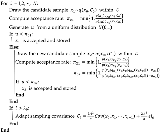
The combination of DR and AM results in the DRAM algorithm. DRAM takes advantage of DR and AM to speed up convergence and enhance the acceptance rate of samples. The intuition in DRAM is to automatically learn information from the chain path and adaptively train the proposal to fit the target posterior. DR and AM in DRAM work jointly and have different functions. For instance, DR allows us to locally adapt the proposal based on rejected samples at each time step. AM allows us to globally adapt the proposal based on previously accepted samples. Given a non-adaptation period of and the initial covariance , a direct way to combine AM and DR is given as follows [18].
- 1.
- Proposal Covariance Adaptation
The proposal covariance at DR’s first stage is adapted using AM, such as computed by current samples in the chain using Equation (16), whenever samples are accepted.
- 2.
- Scaling Parameter
For the i-th DR stage, the covariance is always computed as a scaled version of that in the first stage: , where the scaling parameter can be freely selected. Larger scaling parameters are favored at earlier stages and gradually decrease.
While DRAM incorporates the AM strategy, it can still be challenging to adapt the proposal if the initial covariance is too large, as this deviation prevents the AM process from starting. To address this, the covariance is progressively reduced at higher DR stages, allowing more samples to be accepted and enabling the proper activation of AM. Detailed explanations of DRAM and its hyper-parameters are provided in Haario et al. [18]. For simplicity, this study considers a two-stage DR. The implementation of DRAM is described in Algorithm 1.
| Algorithm 1: DRAM [18] |
| # Initialization |
| : the No. of iterations; : the length of non-adaptation period; |
| , : initial value and covariance, respectively |
| : the proposal distribution |
| : the scaling parameter; : the parameter bounds; : a trial constant : the d-dimensional identity matrix |
 |
3.2. Transitional Markov Chain Monte Carlo (TMCMC)
3.2.1. Concept of TMCMC
To enhance the sampling efficiency of MH, Beck and Au [16] proposed the generation of samples from a sequence of distributions that approach the target posterior rather than directly sampling from the nontrivial target distribution. A kernel sampling density is sequentially updated based on previous sampling results and then used as a new global proposal. However, a significant disadvantage of this method is that when the dimension is high, substantial samples are required, leading to intensive computational demands. The transitional Markov Chain Monte Carlo (TMCMC) developed by Ching and Chen [19] uses a similar idea, employing a series of intermediate or transitional distributions to generate samples that rapidly converge to the target posterior. Unlike [16], TMCMC does not require kernel density estimation. Instead, the intermediate distributions are autonomously defined based on multiple strategies, such as reweighting, resampling, and adaptive random walk at each level.
3.2.2. Mathematical Formulation
TMCMC constructs a series of simple transitional distributions starting from the prior distribution and converging on the target distribution, which is mathematically expressed as
where j is the transition stage number and m is the total number of transition stages. is the intermediate distribution controlled by tempering parameter that takes values from zero and one. At , the initial stage with zero tempering parameters, the posterior is proportional to the prior . At , the final stage with the unity tempering parameter, the intermediate distribution converges on the target distribution. By progressively increasing toward unity, TMCMC calibrates the intermediate distribution from the prior to the target distribution.
The critical part in TMCMC is the determination of the tempering parameter that controls the shape variation between two successive intermediate distributions. should be chosen so that its variation, , allows the smooth transition from to . The acceptance rate is greatly affected by the selection of . Large variations cause sharp changes in the intermediate distribution, leading to high rejection rates with many abandoned samples. Conversely, extremely small variations imply inefficacious sampling with a 100% acceptance rate as all samples are generated from the same distribution [34]. Therefore, an optimal strategy for is required. Once is determined, samples at stage j can be generated from the previous distribution . Ching and Chen [19] recommend using the coefficient of variation (COV) of the so-called plausibility weight of the sample to determine the optimal , which is defined as
Based on the definition of COV, the COV of plausibility weight is given by
where and are the standard deviation and the mean of , where and (in which N is the number of samples and is parameter dimension). in Equation (19) is a function of the conditional on a known . One could prescribe a threshold to satisfy the requirement ; thus, the optimal for each iteration can be automatically computed. Another way to determine is to minimize the absolute difference between and unity in order to preserve COV as the most unified approach to possible. Thus, we obtain
3.2.3. Implementation and Algorithmic Steps
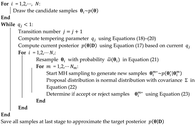
TMCMC starts with sample generation from a prior by any sampling methods at first transition stage, i.e., j = 0 and . As transition continues (j > 0, ), can be calculated based on previously known using Equations (18)–(20). Then, intermediate distribution can be defined. From here, the MH algorithm is applied to generate N samples. To perform resampling at each transition, the normalized plausibility weight is formulated as
Equation (21) allows the resampling of with probability based on available samples from previous intermediate distribution, resulting samples serve as starting MH sampling. The candidate samples are generated from normal distribution with mean and the covariance matrix that facilitates automatic parameter tuning during MH sampling. The covariance matrix is centered at the current samples and expressed as a scaled covariance matrix of intermediate distribution:
in which is a scaling factor that can be determined according to different criteria. One can define as a constant of 0.2 [19] or adaptively tune based on acceptance rates across iterations [48,49]. For the sake of simplicity, is chosen as 0.2 throughout all examples. is the sample mean of weighted samples. Finally, samples are updated recursively by acceptance–rejection with a probability
where is the posterior value at new sample while is calculated at . Throughout all the TMCMC procedures, the tempering parameter is tuned and all steps are repeated until . At final stage, available samples are asymptotically distributed as the posterior .
The key advantage of TMCMC lies in its use of intermediate distributions to avoid the direct sampling of the posterior. At each transition stage, TMCMC generates N samples from a new proposal, enhancing efficiency. Through reweighting, resampling, and the classical MH algorithm, TMCMC avoids the burning-in period, as samples at each stage closely follow the estimated posterior [49]. The algorithmic description of TMCMC is summarized in Algorithm 2.
| Algorithm 2: TMCMC [19] |
| # Initialization |
| : the No. of samples; : parameter dimensions; |
| : initial tempering parameter : prior distribution |
| : a scaling factor of 0.2; |
 |
3.3. Differential Evolution Adaptive Metropolis (DREAM)
Traditional MCMC algorithms adopt a single chain or trajectory to estimate the target posterior. In contrast, DREAM simultaneously employs multiple chains in parallel to explore a global solution. DREAM was originally proposed by Vrugt et al. [50] and consists of two key operations, namely, differential evolution and adaptive randomized subspace sampling, leading to a strong global convergence capability. The differential evolution (DE) allows us to randomly draw sample candidates from multiple chains and enables us to efficiently determine those regions that contain global information. On the other hand, DREAM uses adaptive randomized subspace sampling to automatically tune the mean and variance of the proposal distribution, hence, not relying on artificially selected prior distribution. Building upon multiple chains, DREAM exhibits outstanding performance in estimating high-dimensional and multi-modal posteriors, as multiple chains interactively work on sampling, and the resulting collective information from these chains assists in the concurrently search for multiple local solutions [50].
3.3.1. Differential Evolution in DREAM
The first key component of DREAM is differential evolution (DE), which controls the orientation of sample candidates toward the target posterior. Each Markov chain acts as a source of sample information for the posterior. DE fuses information from multiple chains, enhancing sample quality. Suppose we have the current sample that interacts with samples and from other chains. The proposed sample are generated by DE as follows:
where i is the i-th Markov chain. is the identity matrix, and d is the parameter dimension. and are perturbation values obtained from the d-dimensional multivariate uniform distribution and the d-dimensional multivariate Gaussian distribution , respectively. is the number of considered chain pairs that can gradually increase the default setting of three. is the incremental size of the sample change. and are two vectors containing integers drawn from , N is the number of Markov chains defined in DREAM, and . DREAM defines as one of every five chains that jumps from one posterior to another posterior, resulting in .
3.3.2. Adaptive Randomized Subspace Sampling
In high-dimensional parameter spaces, optimal samples may not be drawn in full dimensions [50]. Adaptive randomized subspace sampling iteratively modifies the proposal variations and updates parameter dimensions based on historical samples. A new subspace is formed by selecting a d-dimensional subset of the parameter space. A crossover probability (CR) determines whether to modify each parameter dimension
where is the d-th dimensional sample of the i-th chain at the (t − 1)-th iteration. is a value sampled from a uniform distribution . is a crossover value that is sampled from a discrete multi-nominal distribution, that is, , where with a different CR for each element in the vector. is the number of CR values and is user-specified. The recommendation of is three by Vrugt et al. [50]. The interpretation of Equation (25) is that the current sample is retained if otherwise, it is updated.
Note that the adaptive randomized subspace sampling strategy is activated when a crossover value , and a vector of sample candidates is then constructed from a multivariate normal distribution. DREAM adaptively tunes the crossover probability by optimizing the distance between two adjacent chains, resulting in a decrease in autocorrelation among the samples in each chain. In particular, when CR = 1, all dimensions are updated; when CR = 0, a single dimension that is randomly selected from d dimensions to avoid the zero value of jump rate is updated.
3.3.3. Detection and Handling of Aberrant Chains
DREAM can detect aberrant chains among multiple chains. Large discrepancies between initial and posterior samples often occur when initial chains use a high-variance prior, slowing convergence. Aberrant chains, stuck in local optima, impair distribution estimates and slow evolution. DREAM uses the inter-quartile range (IQR) method to track abnormal chain status [50]
where and are, respectively, the lower and upper quartiles of the Markov chain computed based on samples before the current time. Chains with are detected as aberrant, and is the mean of the logarithm of the posterior distribution of the last half samples in each chain. Equation (26) serves to ensure each remaining Markov chain is stable from a statistical perspective.
3.3.4. Convergence Evaluation
DREAM evaluates the convergence quality of multiple chains using Gelman–Rubin statistics also known as scale reduction factor [51], as a convergence criterion to determine whether the sampling terminates or not. DREAM algorithm stipulates that if for all unknown parameters, a stable posterior PDF is achieved. is expressed as follows [50]:
where is the number of iteration samples of each chain; is the number of Markov chains used for sampling; is the mean of the variance of total Markov chains; and the ratio of is the variance of the mean of parallel Markov chains. The implementation description of the DREAM algorithm is presented in Algorithm 3.
| Algorithm 3: DREAM [50] |
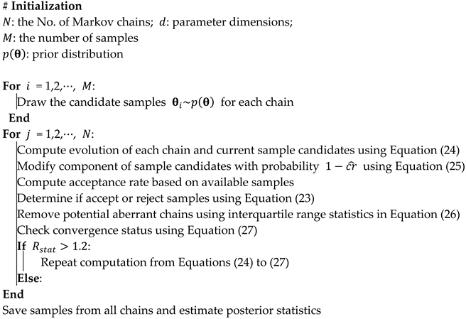 |
It is important to note that the selection of the threshold value of 1.2 for the is based on empirical studies [25,50]. However, determining an appropriate threshold is inherently challenging and may need to be adjusted based on the specific problem at hand. For instance, thresholds of 1.1 or even 1.05 may be more suitable in certain contexts [52]. Gelman et al. [52] also suggest that values below 1.1 are generally acceptable for most applications. Additionally, thresholds can be adaptively adjusted using termination criteria that consider the relationship between the effective sample size (ESS) and the Gelman–Rubin statistic [53]. Discussions on selecting an appropriate threshold can be found in [54,55]. It is crucial to recognize that while is a valuable tool for assessing MCMC convergence, it is not the sole diagnostic measure. Comprehensive diagnostic analysis should include various criteria, such as trace plot visualization, ESS for mixing diagnostics [56,57], and sampler precision [58]. For a more detailed exploration of diagnostic criteria, refer to Gelman et al. [52].
4. Comparative Studies on Numerical Examples
In this Section, the three MCMC algorithms described in Section 3 are applied to Bayesian model updating for structure damage detection. Three engineering structures, namely, a forty-story shear building, a two-span continuous concrete beam, and a pedestrian bridge, are investigated with increasing structural complexity in terms of the number of DOFs. The damage scenarios are intentionally introduced. In all case studies, the performance of each MCMC is evaluated by the accuracy of the damage detection, parameter estimation, and computational cost. It is important to note that the damage scenarios in the numerical examples are intended to represent relative changes in the elastic modulus. For instance, in Table 1, Table 2 and Table 3, a value of −20% corresponds to , where and represent the elastic modulus in the damaged and undamaged conditions, respectively. The decrease in elastic modulus is a common representation of stiffness reduction, as stiffness is directly related to the elastic modulus [24,59,60,61]. Additionally, we define the stiffness parameter (updating parameter) as the ratio of the true elastic modulus (damaged condition) to the nominal elastic modulus (healthy condition). A value of unity indicates an undamaged condition. The values used in our damage scenarios are based on findings from the literature on Bayesian model updating and damage detection in various structures, including laboratory-scaled shear buildings [31,62], steel truss bridges [37], offshore platforms [63], and steel frames [64,65].

Table 1.
Damage location and severity of shear building.
Table 2.
Damage location and severity of concrete beam.
Table 3.
Structural properties and damage scenario of the pedestrian bridge.
Furthermore, the structures analyzed in this study are all based on numerical models. Since the focus of the paper is not on the specific material properties of the structures, we did not specify the material types in detail. For reinforced concrete structures, typical causes of stiffness degradation include cracks, reinforcement corrosion, and localized spalling of concrete, all of which contribute to a reduction in stiffness. In practice, the levels of stiffness degradation used in our model are reasonable and commonly observed in structures that have been in service for extended periods, such as concrete bridges that have been operational for more than a decade. Also, reinforced concrete structures often exhibit cracking during their service life. However, after a prolonged period, these cracks can lead to a degradation in the material’s performance, ultimately reducing the structure’s stiffness. The stiffness reduction assumptions in our study are based on a baseline model representing the structure in its normal service condition. It is important to note that identifying stiffness degradation in reinforced concrete structures does not necessarily imply an imminent collapse. Rather, it highlights a reduction in stiffness that could shorten the structure’s service life or potentially reduce its seismic performance and safety reliability.
As for the specific causes of stiffness reduction, they could be due to a variety of factors such as loose joints/bolts, holes, cuts, cracks, material degradation, or the removal of structural components. However, this study does not focus on the specific causes of stiffness change. Instead, our primary objective is to provide a tutorial on Bayesian model updating using single-chain and multi-chain MCMC, and its application in structural damage detection. We acknowledge that further research into the relationship between damage identification and classification is a valuable area of future study.
In addition, in practical damage detection, a reference or baseline is needed for comparison, meaning measurements should be taken in both the healthy and damaged conditions to accurately distinguish changes in stiffness. In this study, however, the primary focus is a comparative study and tutorial on Bayesian model updating using different MCMC methods. For simplicity, we assume that the baseline model for all examples represents the healthy condition, where all stiffness parameters are in unity. As such, any identified values from the Bayesian model updating (e.g., 0.8 or 0.9) are interpreted as representing the damaged condition.
4.1. A Forty-Story Shear Building
4.1.1. Structural Information for Damage Detection
The 40-DOF shear building shown in Figure 1 is employed as our first example, where the mass per floor and inter-story stiffness are assumed to be uniformly distributed throughout the height. The mass M at each floor is set to 1.2 metric tons, and inter-story stiffness K is set as 356 MN/m. In this example, a total of 40 stiffness parameters corresponding to each floor are updated using measured modal data, i.e., , and the mass properties, i.e., , are well-known and not updated in order to avoid an unidentifiable situation resulting from the coupling effect [66]. We assume that twenty independent measurements are performed. For each measurement, only the first eight natural frequencies and mode shapes are available due to the limited number of sensors and the inaccuracy and difficulty in identifying higher modes. To simulate realistic measurement, Gaussian white noise with zero mean and 1% COV of frequencies and mode shapes is added to exact frequencies and mode shapes [67,68]. The sample variance of each natural frequency and sample covariance matrix of each mode shape in Equation (9) can be calculated using twenty sets of modal data.

Figure 1.
Forty-story shear building and 40-DOF model.
In addition, mode shapes are usually incomplete with missing components; that is, only a few DOFs at test points are measured, as practical measurement is usually taken at restricted locations. For the purpose of vibration-based Bayesian model updating and damage detection, it is beneficial to expand reduced mode shapes onto complete mode shapes with full DOFs. In this example, multiple measurement setups are designed to identify full modal shapes by assembling local ones. Figure 2 schematically shows the setup plan. The 40 DOFs are covered by three setups, each sharing four reference sensors and including twelve rover sensors. Partial/local modal shapes corresponding to different measurement setups contain 12 components related to 12 DOFs. The acquired local mode shapes are then assembled to obtain global mode shapes with 40 DOFs using the least squares method [69].
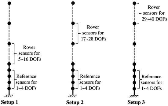
Figure 2.
Setup plan for the shear building.
In this example, a single damage scenario with multiple damaged locations is intentionally introduced, as shown in Table 1. The negative sign indicates the stiffness reduction. Herein, we define the 40 stiffness parameters from the bottom to the top floor, and each parameter is a ratio of true stiffness to nominal stiffness (356 MN/m). Hence, the ground truths of other parameters at undamaged locations are in unity. The first eight natural frequencies and modal shapes corresponding to the damage scenario are used for damage detection with DRAM, TMCMC, and DREAM.
4.1.2. Results
The initialization of DRAM, TMCMC, and DREAM is specified as follows. For DRAM, the initial covariance is defined as a 40-dimensional unit diagonal matrix scaled by a factor of 0.05. The parameter dimension in this example is 40, as recommended by Haario et al. [18], and when the number of dimensions exceeds 20, the non-adaptation period for AM can be taken as 1000. Otherwise, it is taken as 200. The two-stage DR process is implemented with a scaling parameter of 0.1. The initial values for all unknown parameters are set to unity (1), and a sample size of 40,000 is generated. For TMCMC, this example sets the lower and upper bounds of uncertainty parameters as 0.7 and 1.2, respectively. The length of the Markov chain is set as 40,000. The scaling factor in Equation (22) is defined as a default value of 0.2. For DREAM, ten Markov chains are used in parallel to sample parameters. Each chain has a length of 40,000. The initial sample population is generated by a Latin hypercube . Other parameters in DREAM are used as default settings as suggested by Vrugt et al. [50], e.g., in Equation (25). Figure 3, Figure 4 and Figure 5 illustrate the resulting trace plots by DRAM, TMCMC, and DREAM for all uncertainty parameters. It can be observed that all stiffness parameters are estimated to be approximately one by DRAM, indicating that DRAM fails to accurately localize and quantify damage scenarios. A reason for this is due to DRAM’s incapability of dealing with high-dimensional problems, which also corresponds with the conclusion in Vrugt et al. [50]. Furthermore, the performance of DRAM heavily depends on the choice of initial values [70]. For instance, the initial value of unity estimates all parameters as being close to unity in this example.

Figure 3.
Trace plots by DRAM: (a) parameters at undamaged locations; (b) parameters at damaged locations.
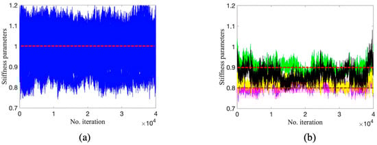
Figure 4.
Trace plots by TMCMC: (a) parameters at undamaged locations; (b) parameters at damaged locations (red dashed line is true value).

Figure 5.
Trace plots by DREAM: (a) parameters at undamaged locations; (b) parameters at damaged locations (red dashed line is true value).
In contrast, it can be found in Figure 4 and Figure 5, where dashed lines denote the true values, that TMCMC and DREAM exhibit better damage detection performance than DRAM. It can be seen that samples using the two methods quickly reach a stationary state, displaying satisfactory convergence. However, two parameters in TMCMC at damaged locations converge to around 0.9 in Figure 4b (black and green trace plots), implying deviation from true values in Table 1. The estimation of all parameters at damaged locations by DREAM in Figure 5b has a desirable agreement with the ground truth in Table 1. Figure 6 shows the trace plots of five Markov chains for four parameters at damaged locations. It can be observed that each Markov chain consistently exhibits fast convergence to the true values, demonstrating the collective power in sampling by DREAM due to the interaction of multiple chains.

Figure 6.
Trace plots of five Markov chains by DREAM: (a) ; (b) ; (c) ; (d) .
Figure 7 shows the marginal distributions of unknown model parameters using the last 10,000 samples obtained by TMCMC and DREAM. Note that the results by DRAM are not included in Figure 7, as all model parameters are estimated as being in unity by DRAM. In addition, for a clear visualization, only parameters at damaged locations, e.g., , , , and , and two parameters at undamaged locations, e.g., , , and , are manifested. It is revealed that the true values consistently cross posterior distributions at a diagonal by DREAM, illustrating a fairly good match between posterior means and true values. On the other hand, the posterior distributions by TMCMC noticeably deviate from true values for certain parameters, e.g., , , and , indicating that TMCMC may provide false alarms for damage detection. It can also be observed that the distributions of , , and are spread across a relatively wide region, suggesting larger uncertainties surrounding these parameters, which is also reflected by significant fluctuations in Figure 4a and Figure 5a.
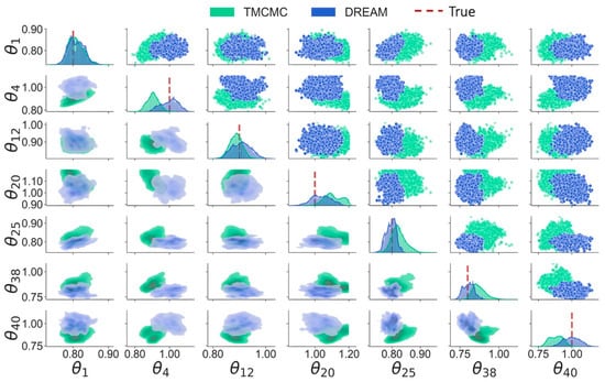
Figure 7.
Marginal distributions of model parameters.
Figure 8 compares the error of parameter estimation by DRAM, TMCMC, and DREAM. It was found that DRAM performs worst in damage detection, giving the maximum error of about 25%. It is worth mentioning that in DRAM, small errors for parameters at undamaged locations mainly arise from the initial value of unity. TMCMC offers acceptable damage detection results for most parameters, but the maximum error is still around 15%, e.g., in and , while DREAM works the best in damage detection with a maximum error of 4.8%, demonstrating that DREAM has superior identification capabilities for high-dimensional problems (40 model parameters), which is attributed to the use of multiple chains to sufficiently explore parameter space.
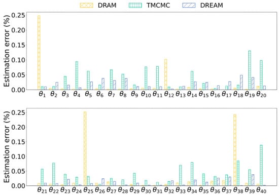
Figure 8.
Estimation error by DRAM, TMCMC, and DREAM.
For the computation of the three algorithms DRAM, TMCMC, and DREAM, we used a personal MacBook, 2017, with a 3.1 GHz Dual-Core Intel Core i5. For 40,000 function evaluations (sample size), DRAM took around 15 min to sample all parameters, although the results of the damage detection were unacceptable. The time spent for damage detection by TMCMC was about 8 min. DREAM displayed the best performance in damage detection, which took around 40 min of computational time. It is understandable that the time elapsed for damage detection is substantially longer when running multiple Markov chains compared to running a single Markov chain. This indicates that the entire computation cost is dependent on each algorithm mechanism and there is a tradeoff between efficiency and accuracy in terms of damage detection.
4.2. Two-Span Continuous Concrete Beam
4.2.1. Structural Information for Damage Detection
A more complex structure with more DOFs than a shear building, a laboratory-scale two-span continuous concrete beam, shown in Figure 9, was used to further numerically investigate the performance of the three MCMC algorithms [71]. Each beam span has a length of 1.9 m. The entire structure was modeled using 30 Euler–Bernoulli elements with thirty-one nodes and three simply supported boundary conditions in MATLAB. This means there are 58 DOFs in total. The cross-sections are 150 mm × 250 mm. The elastic modulus of concrete is 28 GPa. The detailed structural information can be found in [71]. In this example, only transitional DOFs are assumed to be measured due to the difficulty in measuring rotational DOFs. For the 40-story shear building, twenty independent measurements were designed to identify modal data, each containing eight natural frequencies and mode shapes. To achieve element-level damage detection, 30 stiffness parameters corresponding to each beam element, denoted as from left to right in Figure 9b, were chosen to be updated by three algorithms. For each stiffness parameter, the ratio of true elastic modulus to nominal elastic modulus provides the value of unity for parameters at intact elements.

Figure 9.
Two-span continuous concrete beam: (a) specimen in lab; (b) FE model.
Similar to the first example, a three-measurement setup strategy was employed to identify the full modal shape for each independent measurement. As depicted in Figure 10, each setup encompasses 4 reference sensors and 8 rover sensors to cover 28 transitional DOFs. The resulting local mode shapes from each setup were assembled using a least squares method for global mode shapes with 28 components related to 28 DOFs. The eight natural frequencies and mode shapes were added with 1% COV for the purpose of measurement noise consideration. In this example, a multi-damage diagnosis is performed, as shown in Table 2. Multi-damage locations and various damage severities would definitely increase difficulties in damage detection. The damage scenarios in Table 2 are designed to reflect relative changes in the elastic modulus, which could result from various damage sources beyond just cracks. We did not specifically investigate the exact cause of stiffness reduction in these scenarios. Additionally, the design of these damage scenarios is informed by the literature on damage detection in beam structures [71,72,73].
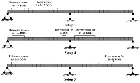
Figure 10.
Three-measurement setup for a concrete beam.
4.2.2. Results
For the implementation of the three algorithms, a sample size of 40,000 samples was set to ensure the sufficient convergence of parameter estimation. The settings of DRAM, TMCMC, and DREAM are identical to those in Section 4.1.
Figure 11, Figure 12 and Figure 13 show the trace plots of 30 stiffness parameters by DRAM, TMCMC, and DREAM. It can be observed that the 30-parameter Markov chains by DRAM in Figure 11 appear to be a phenomenon of ‘sampling stagnation’, in which trace plots consist of many smooth segments, leading to a large rejection rate of candidate samples. This phenomenon is mainly caused by large proposal variances. In addition, the samples of most parameters are not updated until the end of iterations (also referred to as the ‘standing still’ phenomenon) and converge around unity. This may be explained by the fact that (1) DRAM cannot effectively adjust proposal variances for high-dimensional problems, although it combines DR and AM strategies; and (2) as a first example, the initial values greatly affect the performance of DRAM based on the observation that most parameters are estimated to be close to the initial value of unity. It therefore can be concluded that, in this example, DRAM is unable to accurately estimate parameters and detect damage given available modal data.
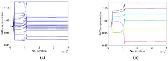
Figure 11.
Trace plots by DRAM: (a) parameters at undamaged locations; (b) parameters at damaged locations.

Figure 12.
Trace plots by TMCMC: (a) parameters at undamaged locations; (b) parameters at damaged locations (red dashed line is true value).

Figure 13.
Trace plots by DREAM: (a) parameters at undamaged locations; (b) parameters at damaged locations (red dashed line is true value).
On the other hand, it can be seen from Figure 12 and Figure 13 that the Markov chains obtained through TMCMC and DREAM continue to fluctuate during the process of sampling and do not exhibit the phenomenon of ‘sampling stagnation’ or ‘standing still’, indicating the generation of valid candidate samples. It can also be seen that the TMCMC has a faster convergence to a stable state compared to DREAM. However, the samples of some parameters at damaged locations significantly diverge from the true values, see the green and cyan samples in Figure 12b, while the Markov chains by DREAM start to converge at around 110,000 iterations. Ultimately, samples of all 30 stiffness parameters fluctuate in close proximity to true values. The slighter fluctuation in Figure 13 compared to those in Figure 12 also illustrates smaller uncertainty and more reliability in parameter estimation using DREAM. Figure 14 displays the sampling process of five Markov chains using DREAM for stiffness parameters at damaged locations. It can be seen that each chain consistently converges to a similar value with another, which also proves the reliability of damage detection by DREAM.

Figure 14.
Trace plots of five Markov chains by DREAM: (a) ; (b) ; (c) ; (d) ; (e) ; (f) .
The marginal posterior distributions of model parameters are shown in Figure 15. Note that only the stiffness parameters at damaged elements, e.g., , , , , , and , and one stiffness parameter at intact elements, e.g., , are present for the sake of brevity. The results of DRAM are ignored in Figure 15 due to its inability to achieve high-dimensional parameter estimation. As observed, all diagonal distributions obtained by DREAM cover the ground truth, while TMCMC results in remarkable deviations of parameter estimation, such as and . In addition, the scatter plots in the upper triangle of TMCMC are more widespread compared to those in DREAM, implying that the resulting samples by TMCMC encompass larger uncertainties, which is also reflected by the trace plots exhibiting greater fluctuations in Figure 12 compared to those in Figure 13. A comparison of the estimation errors of the three algorithms is reported in Figure 16. DRAM performs worst for damage detection, giving a maximum error of over 40% and completely incorrect detection. The estimation error using TMCMC is up to around 10%. DREAM shows the best performance in damage detection, and its maximum estimation error is less than 5%. The results of damage detection demonstrate that the samples obtained by DREAM with fusing information from multi-chains have higher convergence accuracy. The interactions between Markov chains allow the enhancement of the quality of posterior samples.
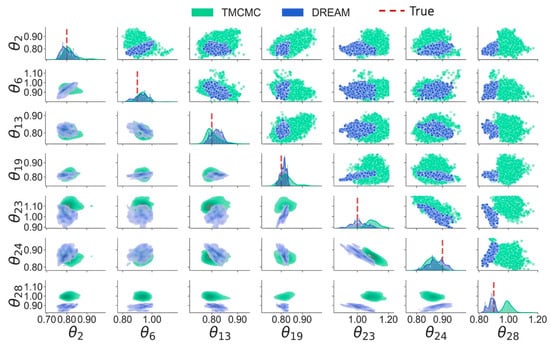
Figure 15.
Marginal distributions of model parameters.
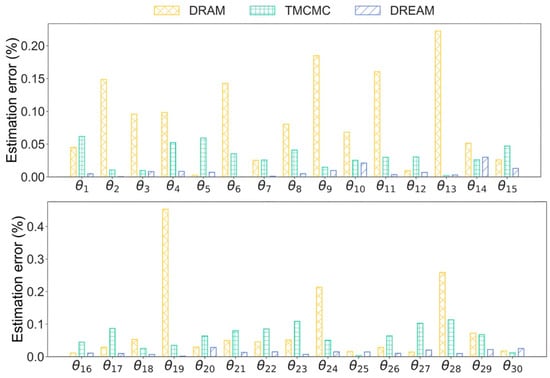
Figure 16.
Estimation error by DRAM, TMCMC, and DREAM.
For computation, the three algorithms were implemented on the same personal laptop. DRAM is the least computationally costly, only requiring about 10 min to evaluate a model 40,000 times. TMCMC takes around 14 min, and DREAM requires the most intensive computational cost of around 50 min for damage detection. The high accuracy of damage detection by DREAM comes with high computational time, as it runs many Markov chains simultaneously in order to seek the best solutions and offer more possibilities and robustness.
4.3. Steel Pedestrian Bridge
4.3.1. Structural Information for Damage Detection
A large-scale steel pedestrian bridge is considered a benchmark in the study of validating the performances of DRAM, TMCMC, and DREAM in terms of parameter estimation and damage detection. The bridge is located on the Georgia Institute of Technology campus and has a height, width, and longitudinal length of 2.74 m, 2.13 m, and 30.17 m, respectively. The FE model of the pedestrian bridge was constructed in SAP 2000, consisting of 46 nodes and 274 DOFs. Figure 17b shows the bridge model and sensor configuration. Seven uniaxial and biaxial accelerometers were installed on the bridge to, respectively, measure vertical and vertical–transverse vibration responses at 21 out of 274 DOFs. The entire structure was divided into six substructures, including frame members and truss members. More detailed model information is provided in [74,75].
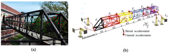
Figure 17.
Three-dimensional pedestrian bridge: (a) pedestrian bridge on the Georgia Tech campus; (b) bridge model and sensor layout.
Table 3 lists the structural properties of the pedestrian bridge, and the damage scenario considered in this study is represented by a reduction in the elastic modulus. and denote the elastic modulus of the frame members and truss members in each substructure. and are four spring stiffnesses representing the boundary conditions. In total, there are 15 stiffness parameters to be updated, denoted as ~, which correspond to , , , and . The damage scenario column in Table 3 lists the relative stiffness variation in the true modulus from its nominal value. For example, and . Here, the values of −0.2 and 0.2 denote a stiffness reduction and increase, respectively. In this example, twenty independent measurements were conducted, each identifying five natural frequencies and modal shapes to perform damage detection. A 1% COV was added to the modal data to simulate a common noise level.
It is worth mentioning that unlike a shear building and concrete beam, which involve multiple measurement setups, each independent measurement in the bridge example only contains a single setup to cover 21 DOFs, as we did not execute element-level damage detection for the pedestrian bridge. In practice, the realization of damage detection at the element level was our ultimate target. However, challenges arose as (1) nontrivial model parameterization was required, that is, assigning a parameter to each element; and (2) the identification of too many parameters was unfeasible due to limited measurement information. Although it is a longstanding problem, the practical method is to separate the entire structure into a few substructures, which are assigned to one parameter. Narrowing down damage to the substructure level is desirable, as inspectors can detect potentially damaged substructures and decide whether they need repair, which is economical and time-saving, rather than checking all individual elements one by one.
The damage severity presented in Table 3 is also consistent with values found in other studies on damage detection in steel bridges [37,76,77]. For this structure, a more appropriate interpretation of the damage scenario would be the reduction in the moment of inertia or stiffness in specific subregions. In practice, changes in the moment of inertia may occur when the geometric configuration of certain regions deviates from the original design, or due to loosening of diagonal bracing in some subregions. Such changes can indeed lead to significant variations in the moment of inertia, potentially by as much as 30% or more, as shown in references [37,76,77]. It is important to emphasize that when analyzing a real structure, it would indeed be necessary to carefully consider the actual types of damage in order to ensure that the damage identification has true physical meaning.
It is worth mentioning that the support spring stiffness is also considered an updating parameter. In Table 3, we account for a 20% increase in the supporting stiffness, which is not necessarily a result of structural damage. It is indeed possible for the spring stiffness to increase under certain conditions. For instance, this could occur due to repairs or reinforcements in the support structure, changes in the boundary conditions, the addition of stiffer materials, or structural modifications that lead to a more rigid connection. The design of the stiffness variation in the supporting spring in Table 3 is based on studies [60,61,78,79].
4.3.2. Results
To implement DRAM, TMCMC, and DREAM, the algorithm settings are identical to those given in Section 4.1 and Section 4.2, except for a setting where a sample size of 15,000 with fewer parameters to be updated was designed. The lower and upper limits of the 15 parameters are set as 0.5 and 1.5, respectively. The trace plots of 15 stiffness parameters for three algorithms are shown in Figure 18, Figure 19 and Figure 20. It can be seen that the Markov chains of all parameters obtained by DRAM appear to be noticeable segments with stagnation and the phenomenon of ‘standing still’, indicating a very low acceptance rate during sampling and leading to the mis-estimation of stiffness parameters. Turning our attention to Figure 19 and Figure 20, the samples of all parameters fluctuate in the vicinity of the true values (red dashed lines), demonstrating a satisfactory convergence using TMCMC and DREAM. It was also found that TMCMC reaches convergence faster than DREAM, mainly because the intermediate distribution in TMCMC reaches the target posterior at an early stage. Figure 21 displays the trace plots of five Markov chains in DREAM in terms of parameters at damaged substructures. All chains have consistent convergence to the ground truth, proving robust and reliable parameter estimation using DREAM.

Figure 18.
Trace plots by DRAM: (a) parameters at undamaged locations; (b) parameters at damaged locations.
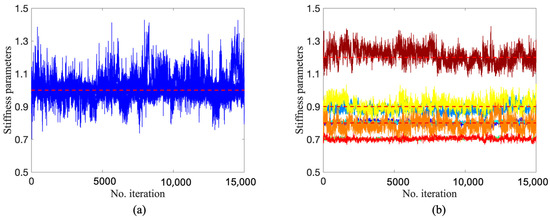
Figure 19.
Trace plots by TMCMC: (a) parameters at undamaged locations; (b) parameters at damaged locations (red dashed line is true value).
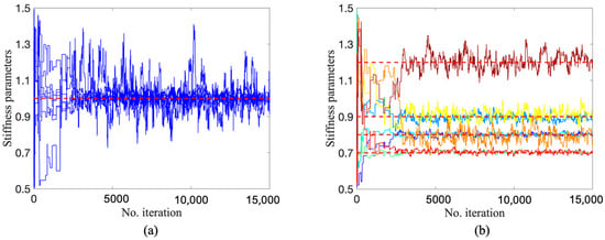
Figure 20.
Trace plots by DREAM: (a) parameters at undamaged locations; (b) parameters at damaged locations (red dashed line is true value).

Figure 21.
Trace plots of five Markov chains by DREAM: (a) ; (b) ; (c) ; (d) ; (e) ; (f) ; (g) ; (h) .
Figure 22 shows the marginal distributions of parameters at damaged substructures obtained by TMCMC and DREAM. As observed, diagonal posterior distributions of the two algorithms are well matched with each other and cover the true values, implying that both algorithms successfully achieve damage localization and quantification but also provide valuable confidence in damage detection. The estimation errors in parameter identification by DRAM, TMCMC, and DREAM are reported in Figure 23. It was found that DRAM gives completely incorrect parameter estimation due to sampling stagnation and sensitivity to initial values, resulting in incorrect damage detection. Conversely, both TMCMC and DREAM exhibit desirable damage detection, probably because of the lower number of to-be-updated parameters compared to previous examples where DREAM always performs best. DREAM slightly outperforms TMCMC; e.g., it has a maximum error of 2% and 6%, respectively. Regarding the computational costs, DRAM only takes around 4 min for sampling but fails to correctly identify parameters. TMCMC takes around 25 min, and DREAM takes the longest, at around 30 min, as multiple Markov chains are concurrently running on the samples.
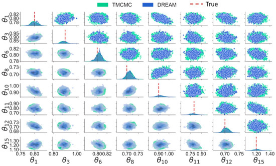
Figure 22.
Marginal distributions of model parameters.
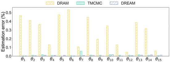
Figure 23.
Estimation error by DRAM, TMCMC, and DREAM.
Table 4 presents a comparative analysis of DRAM, TMCMC, and DREAM and evaluates their performances in terms of accuracy, computational cost, and complexity across a shear building, continuous beam, and pedestrian bridge. In terms of accuracy, DRAM exhibits the lowest values across all cases, indicating that while it may be efficient, it struggles with accurate damage detection and parameter estimation. TMCMC provides medium accuracy, suggesting it offers a balanced approach. While there are noticeable errors between the estimated and true parameters, the level of damage detection remains acceptable. DREAM achieves the highest accuracy, excelling in both damage detection and parameter estimation, offering the precise identification of structural damage. Regarding computational cost, DRAM is the most computationally efficient, requiring the least amount of time. However, this efficiency comes at the cost of lower accuracy. TMCMC falls in the middle regarding computational cost. It strikes a balance between accuracy and computational efficiency. DREAM is the most computationally costly. This higher computational cost correlates with its superior accuracy.
Table 4.
Comparison among DRAM, TMCMC, and DREAM.
The complexity of the algorithms also plays a significant role in their performance. Both DRAM and TMCMC operate using a single chain for sampling, which contributes to their lower computational cost but limits their accuracy. DREAM, on the other hand, utilizes multiple chains, enhancing accuracy but also increasing computational cost. The use of multiple chains allows DREAM to explore the parameter space more thoroughly. Each chain can sample from different regions of the parameter space, reducing the risk of becoming trapped in local optima and increasing the chance of finding the global optimum. This thorough exploration leads to higher accuracy in damage detection and parameter estimation. However, running multiple chains simultaneously requires significantly more computational resources, resulting in higher computational costs.
4.4. Discussion
Three MCMC algorithms are applied to three engineering structures with increasing complexity. This Section discusses the performance of each algorithm in the context of damage detection based on a comparative study.
DRAM has a very easy-to-understand algorithm mechanism and a relatively simpler implementation compared to TMCMC and DREAM, leading to the least computational cost. The settings for implementation include the design of the DR stage, e.g., scaling factor and number of the DR stage, and the design of the AM stage, e.g., a non-adaptation period, as well as initial samples. Through all application cases, it can be seen that DRAM is ineffective in sampling (e.g., sampling stagnation) for high-dimensional problems, mainly owing to the random walk principle. The DRAM would encounter arduous convergence challenges for the target posteriors with complex geometry. DRAM’s capability is greatly limited by the choice of DR and AM or other tuning parameters. A more appropriate DR and AM strategy design would be more beneficial to parameter estimation. Unfortunately, to the best of the authors’ knowledge, there are no comprehensive guidelines for DR and AM. A possible remedy is to tune the DR and AM processes in a trial-and-error manner with user interaction in practice. In addition, it was observed that the selection of initial samples significantly affects the DRAM’s performance on parameter estimation, as shown in Figure 3 and Figure 11. One solution for this shortcoming is to determine better initial samples using global optimization methods, e.g., heuristic optimization [80].
TMCMC generates samples from a series of transitional distributions and has better capabilities for effectively sampling from high-dimensional posteriors compared to DRAM. For moderately high dimensions, e.g., 15 dimensions in Section 4.3, the accuracy of damage detection is acceptable. Nevertheless, for a higher dimensional problem, e.g., 40 dimensions in Section 4.1, its accuracy substantially degrades, even providing misguiding results for damage detection. Among the three sampling algorithms, TMCMC has the fastest convergence speed. In other words, the dropping burn-in period is not an issue in TMCMC. This is attributed to the fact that the initial sample pool in the TMCMC algorithm is directly built based on the prior distribution of model parameters, which bypasses sampling from outside the posteriors. However, the burn-in period may occur in some situations in which the target posterior is very complex and high-dimensional or is distributed over a relatively narrower region [34]. The disadvantages of TMCMC mainly lie in algorithm complexity. The computational cost required in the entire sampling process is more expensive than the process using DRAM. TMCMC does not generate samples from the target posteriors but from intermediate distributions, which means that more parameters at each iteration, e.g., mean and covariance matrix in Equation (22), need to be iteratively tuned. Another problem in TMCMC is the selection of the scaling parameter which is not universal, although it has been suggested as 0.2 in [19]. However, a value of 0.2 may not be optimal and applicable for all cases. A remedial option is to adaptively tune based on the comparison between the mean acceptance rate and target acceptance rate [34].
DREAM employed multiple Markov chains in parallel and differential evolutions as well as randomized subspace strategies in order to sample the posterior distributions. As observed in all demonstration examples, DREAM exhibits the most accurate and reliable performance of damage detection among all algorithms. DREAM allows the sharing of information from each Markov chain. The information fusion by DREAM’s collective power significantly enhances the convergence accuracy and quality of the posterior samples, leading to the best ability in estimating parameters for high-dimensional problems. The main input required to implement DREAM is a number of Markov chains. Other inputs have been elaborately investigated and are recommended by Vrugt et al. [50]. It was found that default algorithm settings work very well for the presented engineering examples. Another key strength is that the issue of initial values is less of a concern in DREAM, as the initial samples are generated using Latin hypercube samples with a physical parameter bound. However, DREAM’s outstanding capability for approximating complex and high-dimensional posteriors comes at the expense of needing to generate samples from different Markov chains. The sample size is much larger than in DRAM and TMCMC, undoubtedly increasing the computational time for damage detection. The time required by DREAM was consistently the highest among the three sampling algorithms. To alleviate the computational burden, one can turn to the parallel computing of Markov chains. Previous studies have demonstrated the feasibility of the parallel computing of MCMC [81].
4.5. Practical Aspect
In terms of selecting the three advanced MCMC methods for practical application, we suggest employing a sequential implementation strategy for posterior investigation and cross-validation. Begin with the DRAM algorithm. DRAM is advantageous for its computational efficiency and straightforward implementation, making it ideal for preliminary parameter estimation and damage detection. It serves as an excellent starting point, allowing for quick and efficient initial assessments. Following the preliminary assessment with DRAM, we advise transitioning to TMCMC or DREAM for further refinement and validation. TMCMC is recommended for its balanced approach, offering a moderate level of accuracy with reasonable computational costs, thereby serving as an effective means to verify and build upon the initial DRAM results. On the other hand, DREAM should be employed when the highest level of accuracy is required. Although DREAM is computationally intensive, its use of multiple chains enables the thorough exploration of the parameter space, ensuring precise damage detection and parameter estimation, which is particularly beneficial for complex structural analyses.
In summary, initiate the process with DRAM for rapid and efficient preliminary analysis. Then, proceed with TMCMC or DREAM to achieve more detailed and accurate validation. This sequential approach ensures a robust and comprehensive examination of posterior distributions, ultimately providing reliable and precise damage detection results.
It is worth mentioning that the scalability of the discussed MCMC techniques was investigated in three different structural types with increasing complexity, ranging from a 40-DOF shear building to a 274-DOF pedestrian bridge. The computational times for each method are all less than an hour. However, for real-world large-scale engineering structures, FE models typically involve hundreds of thousands of elements and nodes. Evaluating such forward models or likelihood functions can become computationally intensive, with each model potentially taking several minutes to run. Given that MCMC methods typically require around 104 evaluations to ensure convergence, the direct application of Bayesian model updating for these large-scale structures becomes computationally prohibitive.
To address these challenges, developing surrogate models of the expensive forward model presents a viable solution. Surrogate models, such as Kriging models [82], polynomial chaos expansions [83], and neural networks [84], can approximate the behavior of the forward model with significantly reduced computational cost. By employing these surrogate models, the evaluation process is accelerated, making the application of Bayesian model updating in large-scale structures both feasible and practical. While the scalability of MCMC techniques is limited by computational resources and time in the context of large-scale systems, the integration of surrogate models offers a promising pathway to overcome these limitations and facilitate efficient Bayesian model updating for complex engineering structures.
5. Conclusions
Bayesian model updating is well-known for parameter estimation and structural damage detection in engineering structures, as confidence in damage detection can be directly and reasonably provided given the posterior distributions. In Bayesian model updating, MCMC algorithms are used as computational tools to sample from the target posteriors. The performance of MCMC algorithms heavily relies on their own mechanisms. Various MCMC algorithms have been developed and prospered to enhance the accuracy and reliability of the sampling process.
In this comparative study paper, three advanced MCMC algorithms, namely, DRAM, TMCMC, and DREAM, were reviewed and compared. Their concepts and basic mechanisms were introduced, and a comparative study of the damage detection of three different engineering structures with increasing complexity was also thoroughly investigated. DRAM takes advantage of DR and AM strategies, but its effectiveness is still restricted to high-dimensional problems and its strong dependence on the initial values. Of all the examples in this study, DRAM performs most poorly in regard to damage detection. The concept in TMCMC is that a series of intermediate distributions is used to sample from the posterior rather than directly sampling. The results show TMCMC that enables the achievement of desirable parameter estimation for moderate-dimensional problems, e.g., 15 dimensions, while, from the application examples presented, it can be seen that DREAM has the strongest capability in estimating parameters, given that it consistently sampled the target posteriors in the 15, 30, and 40 dimensions at a fairly accurate level. This is attributed to the interactions between Markov chains and randomized subspace sampling. However, it comes with a trade-off between sampling efficiency and computational cost.
The results highlight that DRAM, while computationally efficient, struggles with high-dimensional posteriors due to sampling stagnation and sensitivity to initial samples, making it less suitable for complex structural models. TMCMC performs better in moderately high dimensions but degrades in accuracy for very high-dimensional problems, which can lead to misleading damage detection results. DREAM, on the other hand, consistently provides the most accurate and reliable results, particularly for high-dimensional problems, thanks to its use of multiple Markov chains and differential evolution. In addition, DREAM’s higher computational cost, due to the large sample size required, can be mitigated through parallel computing.
In conclusion, the study’s results suggest that while DRAM and TMCMC offer certain advantages in computational efficiency and simplicity, DREAM stands out for its ability to handle complex, high-dimensional posteriors more reliably. This makes it a strong candidate for use in Bayesian model updating and structural damage detection where precision and robustness are critical. Future work could explore optimizing computational efficiency in DREAM through parallelization or other advanced techniques, making it more applicable to real-world scenarios where high dimensionality is common.
It should be noted that, in this study, all the application examples are numerical, with the final example involving a benchmark study of a steel pedestrian bridge. We simulate realistic measurement conditions by incorporating aspects such as limited data and measurement noise when performing Bayesian model updating and damage detection. As this paper serves as a tutorial on Bayesian model updating with different MCMC methods, our primary focus is on numerically demonstrating Bayesian model updating across different structural types. In future studies, we plan to extend this work by applying Bayesian model updating to practical cases through experimental tests, as part of our ongoing research.
Current Bayesian model updating relies heavily on the evaluation of the likelihood function. However, for complex models, such as multi-level models that embed sub-models, the likelihood function is often intractable and not available in a closed form. Likelihood-free inference (LFI) offers a viable alternative to traditional Bayesian model updating by bypassing the need for explicit likelihood calculations. Emerging techniques like Generative Adversarial Networks [85] and normalizing flows [86,87] can further improve Bayesian model updating and structural damage detection by providing more accurate and computationally efficient approximations of the posterior distributions. Future research will focus on advancing LFI methods and integrating machine learning techniques to overcome the limitations of traditional Bayesian model updating, thereby improving structural damage detection and model updating in complex, large-scale systems.
Author Contributions
Conceptualization, J.Z.; Methodology, L.L., H.C. and J.Z.; Software, H.C. and J.Z.; Validation, H.C. and S.W.; Formal analysis, L.L. and J.Z.; Writing—original draft, L.L. and J.Z.; Writing—review & editing, H.C., S.W. and J.Z.; Funding acquisition, L.L. All authors have read and agreed to the published version of the manuscript.
Funding
Funding for this work was provided by the Scientific Research Project of the Hubei Provincial Department of Education (No. B2022490 and No. B2022491). The support is gratefully acknowledged.
Institutional Review Board Statement
Not applicable.
Informed Consent Statement
Not applicable.
Data Availability Statement
The data and codes used in this study are publicly available and can be accessed at https://github.com/Jice1991 (accessed on 19 September 2024).
Conflicts of Interest
The authors declare that they have no known competing financial interests or personal relationships that could have appeared to influence the work reported in this paper.
References
- Ozcelik, O.; Misir, I.S.; Yucel, U.; Durmazgezer, E.; Yucel, G.; Amaddeo, C. Model updating of Masonry courtyard walls of the historical Isabey mosque using ambient vibration measurements. J. Civ. Struct. Health Monit. 2022, 12, 1157–1172. [Google Scholar] [CrossRef]
- Li, Y.; Tian, K.; Hao, P.; Wang, B.; Wu, H.; Wang, B. Finite element model updating for repeated eigenvalue structures via the reduced-order model using incomplete measured modes. Mech. Syst. Signal Process. 2020, 142, 106748. [Google Scholar] [CrossRef]
- Alkayem, N.F.; Cao, M.; Zhang, Y.; Bayat, M.; Su, Z. Structural damage detection using finite element model updating with evolutionary algorithms: A survey. Neural. Comput. Appl. 2018, 30, 389–411. [Google Scholar] [CrossRef] [PubMed]
- Razavi, M.; Hadidi, A. Structural damage identification through sensitivity-based finite element model updating and wavelet packet transform component energy. In Structures; Elsevier: Amsterdam, The Netherlands, 2021. [Google Scholar]
- Hu, S.-L.J.; Li, H.; Wang, S. Cross-model cross-mode method for model updating. Mech. Syst. Signal Process. 2007, 21, 1690–1703. [Google Scholar] [CrossRef]
- Carvalho, J.; Datta, B.N.; Gupta, A.; Lagadapati, M. A direct method for model updating with incomplete measured data and without spurious modes. Mech. Syst. Signal Process. 2007, 21, 2715–2731. [Google Scholar] [CrossRef]
- Rezaiee-Pajand, M.; Entezami, A.; Sarmadi, H. A sensitivity-based finite element model updating based on unconstrained optimization problem and regularized solution methods. Struct. Control. Health Monit. 2020, 27, e2481. [Google Scholar] [CrossRef]
- Zhu, H.; Li, J.; Tian, W.; Weng, S.; Peng, Y.; Zhang, Z.; Chen, Z. An enhanced substructure-based response sensitivity method for finite element model updating of large-scale structures. Mech. Syst. Signal Process. 2021, 154, 107359. [Google Scholar] [CrossRef]
- Guedria, N.B. An accelerated differential evolution algorithm with new operators for multi-damage detection in plate-like structures. Appl. Math. Model. 2020, 80, 366–383. [Google Scholar] [CrossRef]
- Ghahremani, B.; Bitaraf, M.; Rahami, H. A fast-convergent approach for damage assessment using CMA-ES optimization algorithm and modal parameters. J. Civ. Struct. Health Monit. 2020, 10, 497–511. [Google Scholar] [CrossRef]
- Mares, C.; Mottershead, J.; Friswell, M. Stochastic model updating: Part 1—Theory and simulated example. Mech. Syst. Signal Process. 2006, 20, 1674–1695. [Google Scholar] [CrossRef]
- Katafygiotis, L.S.; Beck, J.L. Updating models and their uncertainties. II: Model identifiability. J. Eng. Mech. 1998, 124, 463–467. [Google Scholar] [CrossRef]
- Liu, P.; Huang, S.; Song, M.; Yang, W. Bayesian model updating of a twin-tower masonry structure through subset simulation optimization using ambient vibration data. J. Civ. Struct. Health Monit. 2021, 11, 129–148. [Google Scholar] [CrossRef]
- Chib, S.; Jeliazkov, I. Accept–reject Metropolis–Hastings sampling and marginal likelihood estimation. Stat. Neerl. 2005, 59, 30–44. [Google Scholar] [CrossRef]
- Cheung, S.H.; Beck, J.L. Bayesian Model Updating Using Hybrid Monte Carlo Simulation with Application to Structural Dynamic Models with Many Uncertain Parameters. J. Eng. Mech. 2009, 135, 243–255. [Google Scholar] [CrossRef]
- Beck, J.L.; Au, S.-K. Bayesian Updating of Structural Models and Reliability using Markov Chain Monte Carlo Simulation. J. Eng. Mech. 2002, 128, 380–391. [Google Scholar] [CrossRef]
- Liang, F.; Liu, C.; Carroll, R. Advanced Markov Chain Monte Carlo Methods: Learning from Past Samples; John Wiley & Sons: Hoboken, NJ, USA, 2011. [Google Scholar]
- Haario, H.; Laine, M.; Mira, A.; Saksman, E. DRAM: Efficient adaptive MCMC. Stat. Comput. 2006, 16, 339–354. [Google Scholar] [CrossRef]
- Ching, J.; Chen, Y.-C. Transitional Markov chain Monte Carlo method for Bayesian model updating, model class selection, and model averaging. J. Eng. Mech. 2007, 133, 816–832. [Google Scholar] [CrossRef]
- Wang, X.; Hou, R.; Xia, Y.; Zhou, X. Structural damage detection based on variational Bayesian inference and delayed rejection adaptive Metropolis algorithm. Struct. Health Monit. 2021, 20, 1518–1535. [Google Scholar] [CrossRef]
- García-Macías, E.; Ubertini, F. Real-time Bayesian damage identification enabled by sparse PCE-Kriging meta-modelling for continuous SHM of large-scale civil engineering structures. J. Build. Eng. 2022, 59, 105004. [Google Scholar] [CrossRef]
- Ding, Y.-J.; Wang, Z.-C.; Chen, G.; Ren, W.-X.; Xin, Y. Markov Chain Monte Carlo-based Bayesian method for nonlinear stochastic model updating. J. Sound Vib. 2022, 520, 116595. [Google Scholar] [CrossRef]
- Yan, W.-J.; Chronopoulos, D.; Papadimitriou, C.; Cantero-Chinchilla, S.; Zhu, G.-S. Bayesian inference for damage identification based on analytical probabilistic model of scattering coefficient estimators and ultrafast wave scattering simulation scheme. J. Sound Vib. 2020, 468, 115083. [Google Scholar] [CrossRef]
- Zhou, X.; Kim, C.-W.; Zhang, F.-L.; Chang, K.-C. Vibration-based Bayesian model updating of an actual steel truss bridge subjected to incremental damage. Eng. Struct. 2022, 260, 114226. [Google Scholar] [CrossRef]
- Vrugt, J.A. Markov chain Monte Carlo simulation using the DREAM software package: Theory, concepts, and MATLAB implementation. Environ. Model. Softw. 2016, 75, 273–316. [Google Scholar] [CrossRef]
- Vrugt, J.A.; Gupta, H.V.; Bouten, W.; Sorooshian, S. A Shuffled Complex Evolution Metropolis algorithm for optimization and uncertainty assessment of hydrologic model parameters. Water Resour. Res. 2003, 39, 1201. [Google Scholar] [CrossRef]
- Ter Braak, C.J. A Markov Chain Monte Carlo version of the genetic algorithm Differential Evolution: Easy Bayesian computing for real parameter spaces. Stat. Comput. 2006, 16, 239–249. [Google Scholar] [CrossRef]
- Calderhead, B.; Girolami, M. Estimating Bayes factors via thermodynamic integration and population MCMC. Comput. Stat. Data Anal. 2009, 53, 4028–4045. [Google Scholar] [CrossRef]
- Laloy, E.; Vrugt, J.A. High-dimensional posterior exploration of hydrologic models using multiple-try DREAM (ZS) and high-performance computing. Water Resour. Res. 2012, 48, W01526. [Google Scholar] [CrossRef]
- Zhou, K.; Tang, J. Computational inference of vibratory system with incomplete modal information using parallel, interactive and adaptive Markov chains. J. Sound Vib. 2021, 511, 116331. [Google Scholar] [CrossRef]
- Zeng, J.; Kim, Y.H. Probabilistic Damage Detection and Identification of Coupled Structural Parameters using Bayesian Model Updating with Added Mass. J. Sound Vib. 2022, 539, 117275. [Google Scholar] [CrossRef]
- Nichols, J.; Moore, E.; Murphy, K. Bayesian identification of a cracked plate using a population-based Markov Chain Monte Carlo method. Comput. Struct. 2011, 89, 1323–1332. [Google Scholar] [CrossRef]
- Wan, H.-P.; Ren, W.-X. Stochastic model updating utilizing Bayesian approach and Gaussian process model. Mech. Syst. Signal Process. 2016, 70–71, 245–268. [Google Scholar] [CrossRef]
- Lye, A.; Cicirello, A.; Patelli, E. Sampling methods for solving Bayesian model updating problems: A tutorial. Mech. Syst. Signal Process. 2021, 159, 107760. [Google Scholar] [CrossRef]
- Der Kiureghian, A.; Ditlevsen, O. Aleatory or epistemic? Does it matter? Struct. Saf. 2009, 31, 105–112. [Google Scholar] [CrossRef]
- Yuen, K.-V. Bayesian Methods for Structural Dynamics and Civil Engineering; John Wiley Sons: Hoboken, NJ, USA, 2010. [Google Scholar]
- Mustafa, S.; Matsumoto, Y. Bayesian Model Updating and Its Limitations for Detecting Local Damage of an Existing Truss Bridge. J. Bridge Eng. 2017, 22, 04017019. [Google Scholar] [CrossRef]
- Sedehi, O.; Papadimitriou, C.; Katafygiotis, L.S. Probabilistic hierarchical Bayesian framework for time-domain model updating and robust predictions. Mech. Syst. Signal Process. 2019, 123, 648–673. [Google Scholar] [CrossRef]
- Das, S.; Saha, P.; Patro, S. Vibration-based damage detection techniques used for health monitoring of structures: A review. J. Civ. Struct. Health Monit. 2016, 6, 477–507. [Google Scholar] [CrossRef]
- Yuen, K.-V. Recent developments of Bayesian model class selection and applications in civil engineering. Struct. Saf. 2010, 32, 338–346. [Google Scholar] [CrossRef]
- Jaynes, E. The relation of Bayesian and maximum entropy methods. In Maximum-Entropy and Bayesian Methods in Science and Engineering; Springer: Berlin/Heidelberg, Germany, 1988; pp. 25–29. [Google Scholar]
- Jaishi, B.; Ren, W.-X. Structural finite element model updating using ambient vibration test results. J. Struct. Eng. 2005, 131, 617–628. [Google Scholar] [CrossRef]
- Jin, S.-S.; Cho, S.; Jung, H.-J.; Lee, J.-J.; Yun, C.-B. A new multi-objective approach to finite element model updating. J. Sound Vib. 2014, 333, 2323–2338. [Google Scholar] [CrossRef]
- Brincker, R.; Ventura, C. Introduction to Operational Modal Analysis; John Wiley & Sons: Hoboken, NJ, USA, 2015. [Google Scholar]
- Green, P.J.; Mira, A. Delayed rejection in reversible jump Metropolis–Hastings. Biome 2001, 88, 1035–1053. [Google Scholar] [CrossRef]
- Haario, H.; Saksman, E.; Tamminen, J. An adaptive Metropolis algorithm. Bernoulli 2001, 7, 223–242. [Google Scholar] [CrossRef]
- Yang, X.-S. Introduction to Algorithms for Data Mining and Machine Learning; Academic Press: Cambridge, MA, USA, 2019. [Google Scholar]
- Lye, A.; Cicirello, A.; Patelli, E. An efficient and robust sampler for Bayesian inference: Transitional Ensemble Markov Chain Monte Carlo. Mech. Syst. Signal Process. 2022, 167, 108471. [Google Scholar] [CrossRef]
- Betz, W.; Papaioannou, I.; Straub, D. Transitional markov chain monte carlo: Observations and improvements. J. Eng. Mech. 2016, 142, 04016016. [Google Scholar] [CrossRef]
- Vrugt, J.A.; Ter Braak, C.; Diks, C.; Robinson, B.A.; Hyman, J.M.; Higdon, D. Accelerating Markov chain Monte Carlo simulation by differential evolution with self-adaptive randomized subspace sampling. Int. J. Nonlinear Sci. Numer. Simul. 2009, 10, 273–290. [Google Scholar] [CrossRef]
- Gelman, A.; Rubin, D.B. Inference from iterative simulation using multiple sequences. Stat. Sci. 1992, 7, 457–472. [Google Scholar] [CrossRef]
- Gelman, A.; Carlin, J.B.; Stern, H.S.; Rubin, D.B. Bayesian Data Analysis; Chapman and Hall/CRC: Boca Raton, FL, USA, 1995. [Google Scholar]
- Vats, D.; Knudson, C. Revisiting the gelman–rubin diagnostic. Stat. Sci. 2021, 36, 518–529. [Google Scholar] [CrossRef]
- Vehtari, A.; Gelman, A.; Simpson, D.; Carpenter, B.; Bürkner, P.-C. Rank-normalization, folding, and localization: An improved R^ for assessing convergence of MCMC (with discussion). Bayesian Anal. 2021, 16, 667–718. [Google Scholar] [CrossRef]
- Du, H.; Ke, Z.; Jiang, G.; Huang, S. The Performances of Gelman-Rubin and Geweke’s Convergence Diagnostics of Monte Carlo Markov Chains in Bayesian Analysis. J. Behav. Data Sci. 2022, 2, 47–72. [Google Scholar] [CrossRef]
- Pasarica, C.; Gelman, A. Adaptively scaling the Metropolis algorithm using expected squared jumped distance. Stat. Sin. 2010, 20, 343–364. [Google Scholar]
- Zitzmann, S.; Weirich, S.; Hecht, M. Using the effective sample size as the stopping criterion in Markov chain Monte Carlo with the Bayes Module in M plus. Psych 2021, 3, 336–347. [Google Scholar] [CrossRef]
- Zitzmann, S.; Hecht, M. Going beyond convergence in Bayesian estimation: Why precision matters too and how to assess it. Struct. Equ. Model. A Multidiscip. J. 2019, 26, 646–661. [Google Scholar] [CrossRef]
- Lombaert, G.; Moaveni, B.; He, X.; Conte, J. Damage identification of a seven-story reinforced concrete shear wall building using Bayesian model updating. In Proceedings of the IMAC-XXVII, Orlando, FL, USA, 9–12 February 2009. [Google Scholar]
- Zhu, D.; Dong, X.; Wang, Y. Substructure stiffness and mass updating through minimization of modal dynamic residuals. J. Eng. Mech. 2016, 142, 04016013. [Google Scholar] [CrossRef]
- Otsuki, Y.; Lander, P.; Dong, X.; Wang, Y. Formulation and application of SMU: An open-source MATLAB package for structural model updating. Adv. Struct. Eng. 2022, 25, 698–715. [Google Scholar] [CrossRef]
- Zhang, Z.; Sun, C.; Guo, B. Transfer-learning guided Bayesian model updating for damage identification considering modeling uncertainty. Mech. Syst. Signal Process. 2022, 166, 108426. [Google Scholar] [CrossRef]
- Fathi, A.; Esfandiari, A.; Fadavie, M.; Mojtahedi, A. Damage detection in an offshore platform using incomplete noisy FRF data by a novel Bayesian model updating method. Ocean. Eng. 2020, 217, 108023. [Google Scholar] [CrossRef]
- Ni, P.; Li, J.; Hao, H.; Han, Q.; Du, X. Probabilistic model updating via variational Bayesian inference and adaptive Gaussian process modeling. Comput. Methods Appl. Mech. Eng. 2021, 383, 113915. [Google Scholar] [CrossRef]
- Yin, T.; Jiang, Q.-H.; Yuen, K.-V. Vibration-based damage detection for structural connections using incomplete modal data by Bayesian approach and model reduction technique. Eng. Struct. 2017, 132, 260–277. [Google Scholar] [CrossRef]
- Zeng, J.; Kim, Y.H. Identification of Structural Stiffness and Mass using Bayesian Model Updating Approach with Known Added Mass: Numerical Investigation. Int. J. Struct. Stab. Dyn. 2020, 20, 2050123. [Google Scholar] [CrossRef]
- Zeng, J.; Xie, Y.-L.; Kim, Y.H.; Wang, J. Automation in Bayesian operational modal analysis using clustering-based interpretation of stabilization diagram. J. Civ. Struct. Health Monit. 2022, 13, 443–467. [Google Scholar] [CrossRef]
- Zeng, J.; Kim, Y.H. A two-stage framework for automated operational modal identification. Struct. Infrastruct. Eng. 2021, 19, 1–20. [Google Scholar] [CrossRef]
- Au, S.-K. Assembling mode shapes by least squares. Mech. Syst. Signal Process. 2011, 25, 163–179. [Google Scholar] [CrossRef]
- Jin, S.-S.; Ju, H.; Jung, H.-J. Adaptive Markov chain Monte Carlo algorithms for Bayesian inference: Recent advances and comparative study. Struct. Infrastruct. Eng. 2019, 15, 1548–1565. [Google Scholar] [CrossRef]
- Wu, Z.; Huang, B.; Chen, H.; Zhang, H. A new homotopy approach for stochastic static model updating with large uncertain measurement errors. Appl. Math. Model. 2021, 98, 758–782. [Google Scholar] [CrossRef]
- Wang, D.; Chen, Z.; Xiang, W.; Zhu, H. Experimental investigation of damage identification in beam structures based on the strain statistical moment. Adv. Struct. Eng. 2017, 20, 747–758. [Google Scholar] [CrossRef]
- Wang, D.; Xiang, W.; Zhu, H. Damage identification in beam type structures based on statistical moment using a two step method. J. Sound Vib. 2014, 333, 745–760. [Google Scholar] [CrossRef]
- Dong, X.; Wang, Y. Formulation and Optimization Algorithm Comparison for the FE Model Updating of Large-Scale Models. 2019. Available online: https://api.semanticscholar.org/CorpusID:174778013 (accessed on 19 September 2024).
- Dong, X.; Wang, Y. Finite element model updating of a steel pedestrian bridge model. In Computing in Civil Engineering 2019: Smart Cities, Sustainability, and Resilience; American Society of Civil Engineers: Reston, VA, USA, 2019; pp. 397–404. [Google Scholar]
- Yin, T.; Zhu, H.-p. Probabilistic damage detection of a steel truss bridge model by optimally designed Bayesian neural network. Sensors 2018, 18, 3371. [Google Scholar] [CrossRef]
- Mousavi, A.A.; Zhang, C.; Masri, S.F.; Gholipour, G. Structural damage detection method based on the complete ensemble empirical mode decomposition with adaptive noise: A model steel truss bridge case study. Struct. Health Monit. 2022, 21, 887–912. [Google Scholar] [CrossRef]
- Li, D.; Zhang, J. Finite element model updating through derivative-free optimization algorithm. Mech. Syst. Signal Process. 2023, 185, 109726. [Google Scholar] [CrossRef]
- Otsuki, Y.; Wang, Y. Finite Element Model Updating of Non-Proportional and Exponential Non-Viscous Damping Systems using Complex Eigenvalues and Eigenvectors. J. Sound Vib. 2024, 589, 118589. [Google Scholar] [CrossRef]
- Rardin, R.L.; Uzsoy, R. Experimental evaluation of heuristic optimization algorithms: A tutorial. JHeu 2001, 7, 261–304. [Google Scholar]
- Yan, W.-J.; Cao, S.-Z.; Ren, W.-X.; Yuen, K.-V.; Li, D.; Katafygiotis, L. Vectorization and distributed parallelization of Bayesian model updating based on a multivariate complex-valued probabilistic model of frequency response functions. Mech. Syst. Signal Process. 2021, 156, 107615. [Google Scholar] [CrossRef]
- Zeng, J.; Kim, Y.H.; Qin, S. Bayesian Model Updating for Structural Dynamic Applications Combing Differential Evolution Adaptive Metropolis and Kriging Model. J. Struct. Eng. 2023, 149, 04023070. [Google Scholar] [CrossRef]
- Novak, L.; Novak, D. Polynomial chaos expansion for surrogate modelling: Theory and software. Beton-Und Stahlbetonbau 2018, 113, 27–32. [Google Scholar] [CrossRef]
- Papadopoulos, V.; Soimiris, G.; Giovanis, D.; Papadrakakis, M. A neural network-based surrogate model for carbon nanotubes with geometric nonlinearities. Comput. Methods Appl. Mech. Eng. 2018, 328, 411–430. [Google Scholar] [CrossRef]
- Creswell, A.; White, T.; Dumoulin, V.; Arulkumaran, K.; Sengupta, B.; Bharath, A.A. Generative adversarial networks: An overview. IEEE Signal Process. Mag. 2018, 35, 53–65. [Google Scholar] [CrossRef]
- Zeng, J.; Todd, M.D.; Hu, Z. A recursive inference method based on invertible neural network for multi-level model updating using video monitoring data. Mech. Syst. Signal Process. 2023, 203, 110736. [Google Scholar] [CrossRef]
- Zeng, J.; Todd, M.D.; Hu, Z. Probabilistic damage detection using a new likelihood-free Bayesian inference method. J. Civ. Struct. Health Monit. 2022, 13, 319–341. [Google Scholar] [CrossRef]
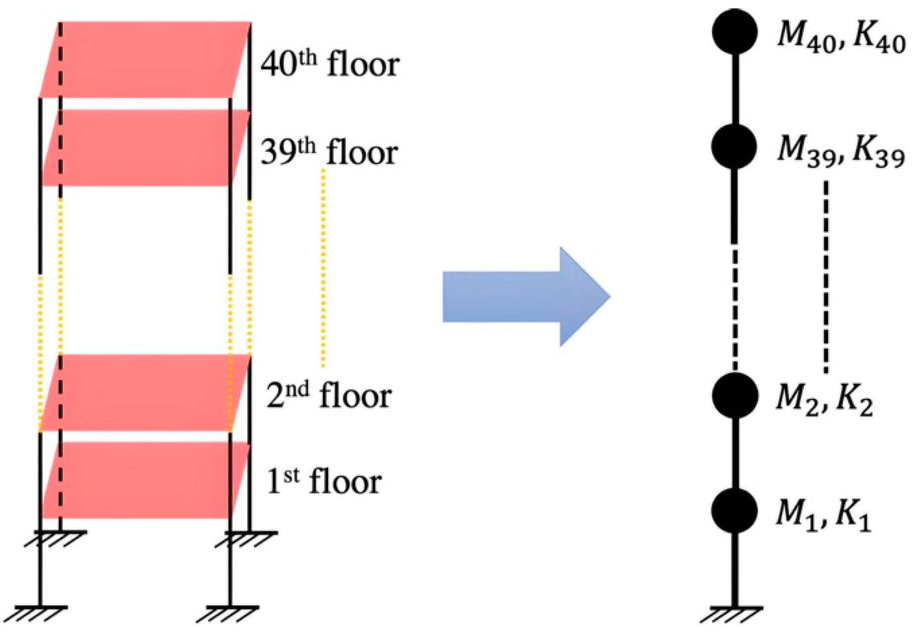
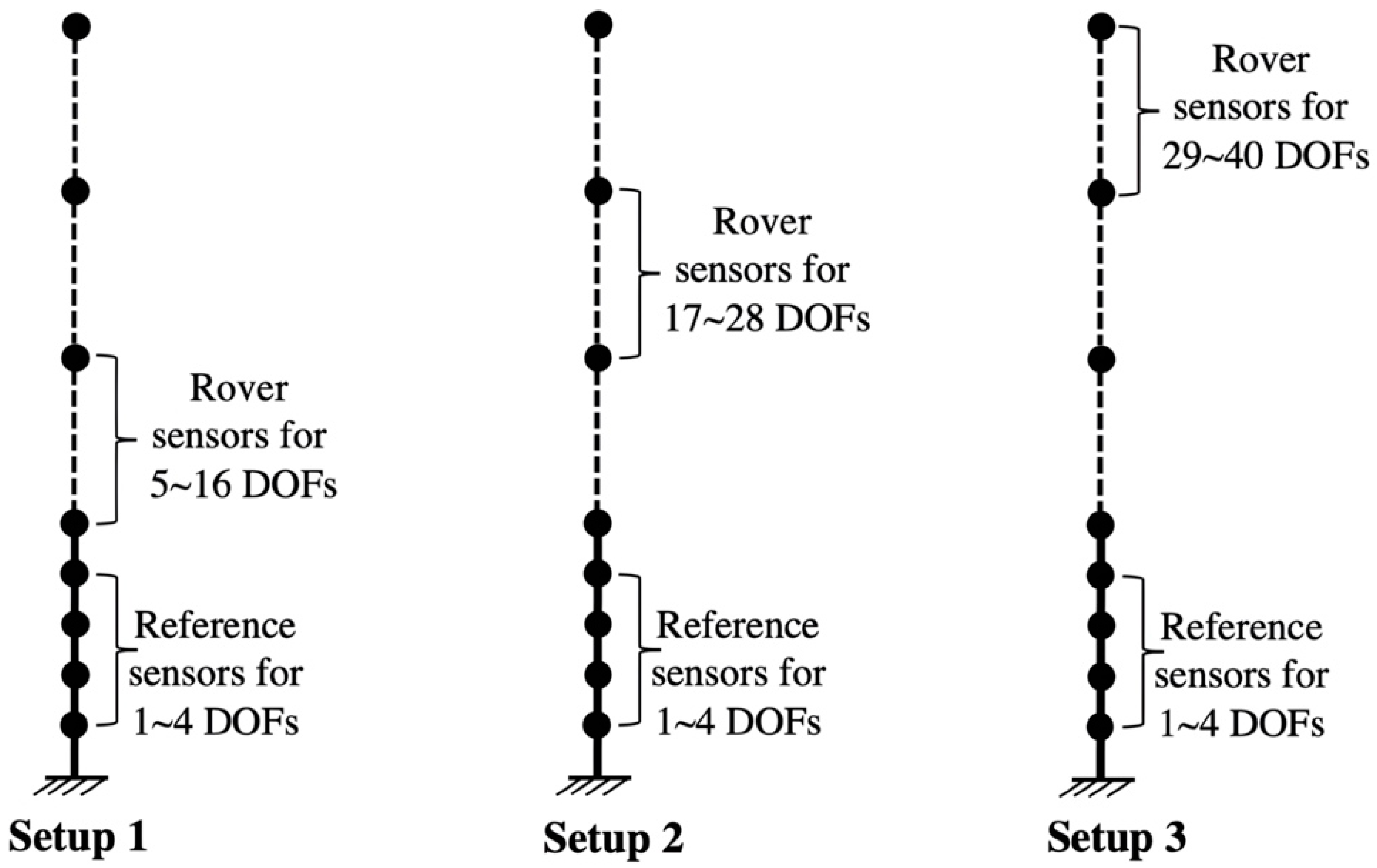
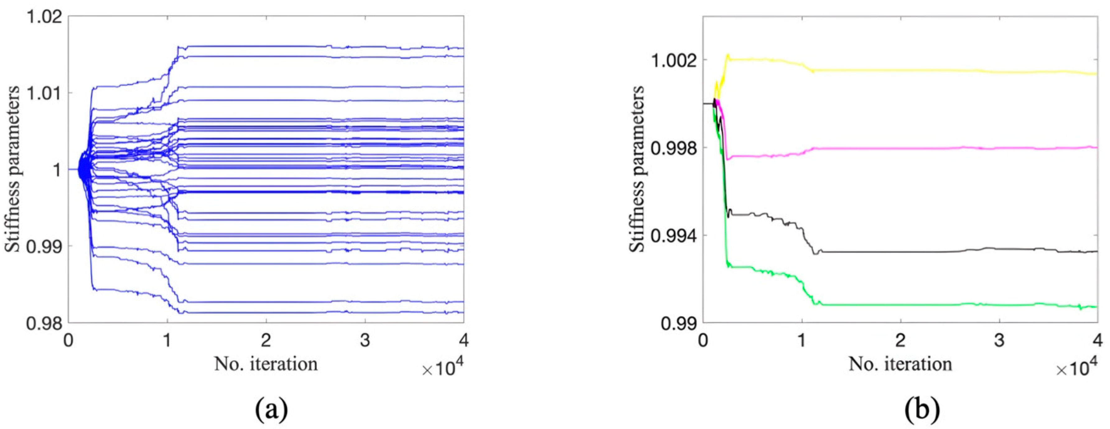
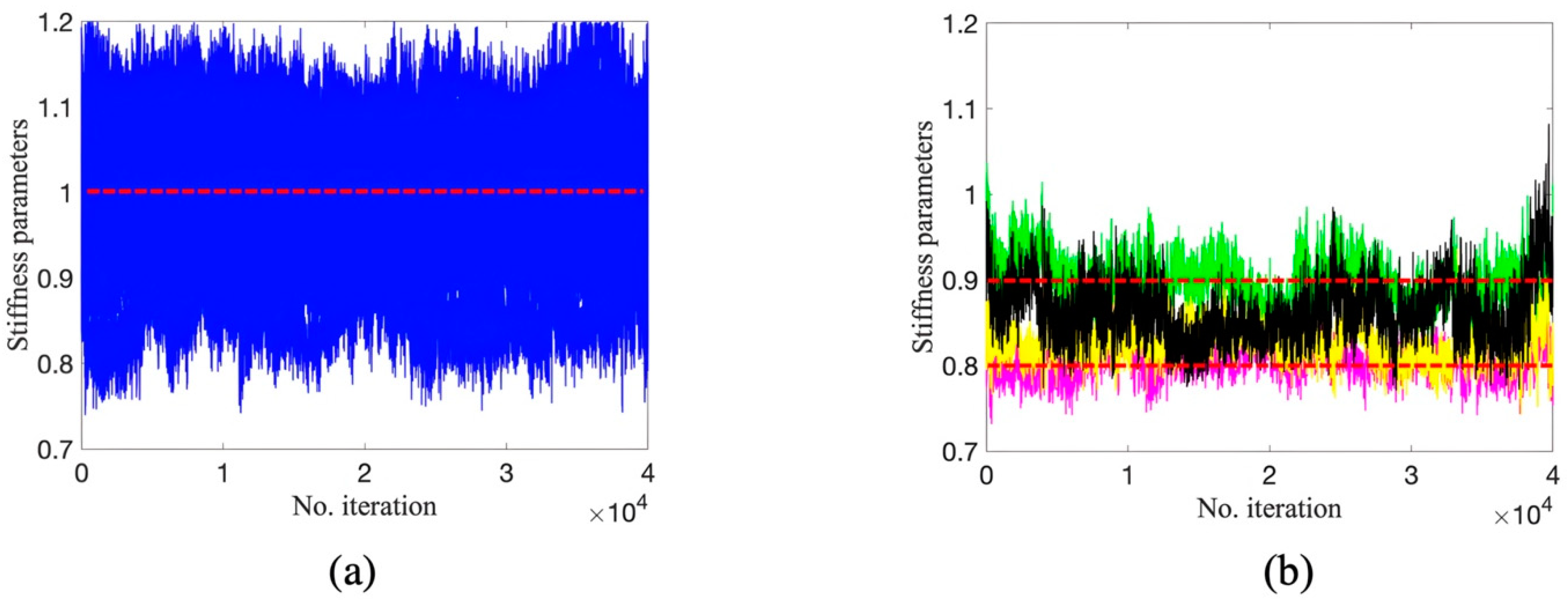
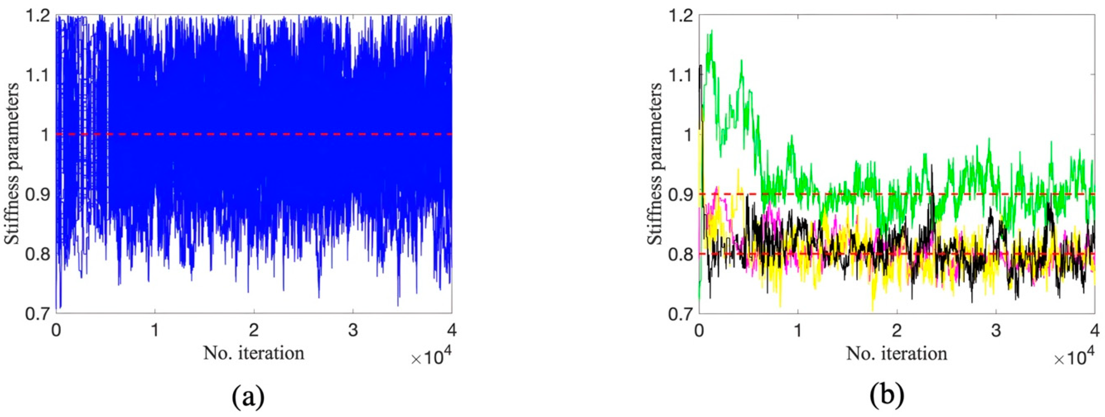
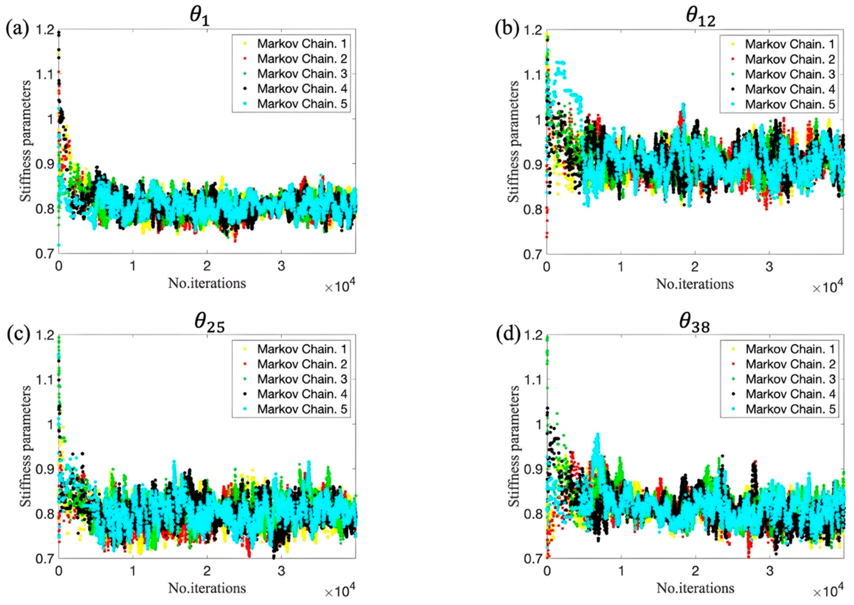


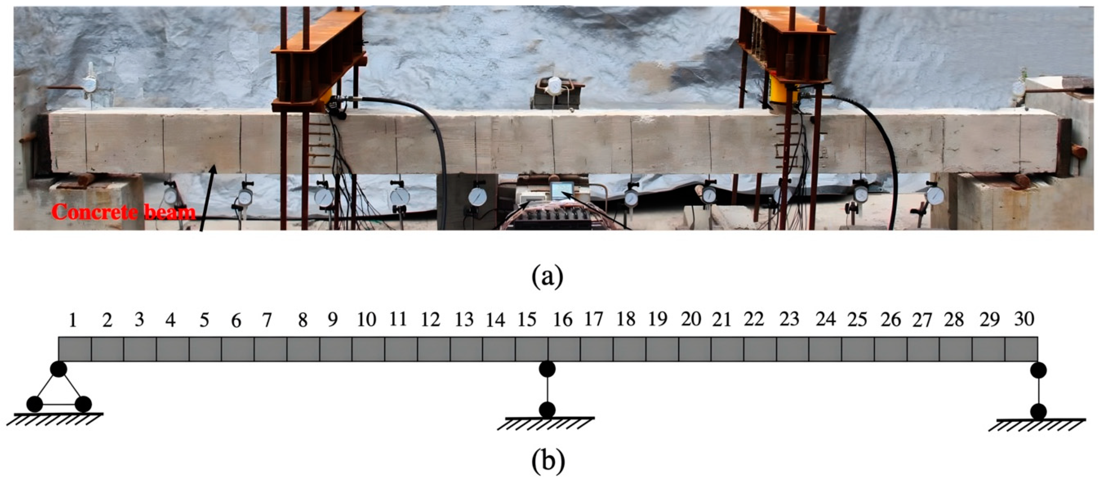
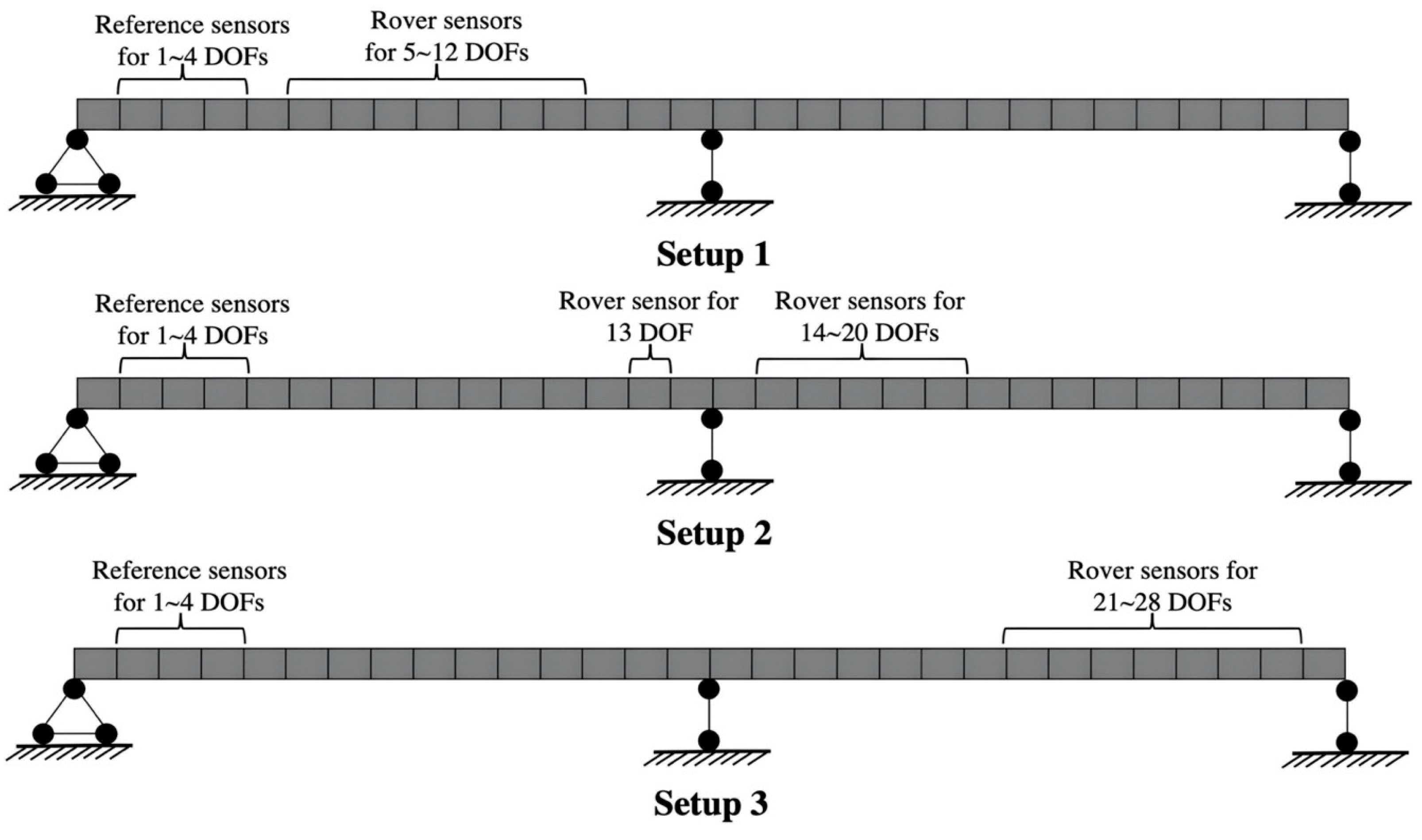
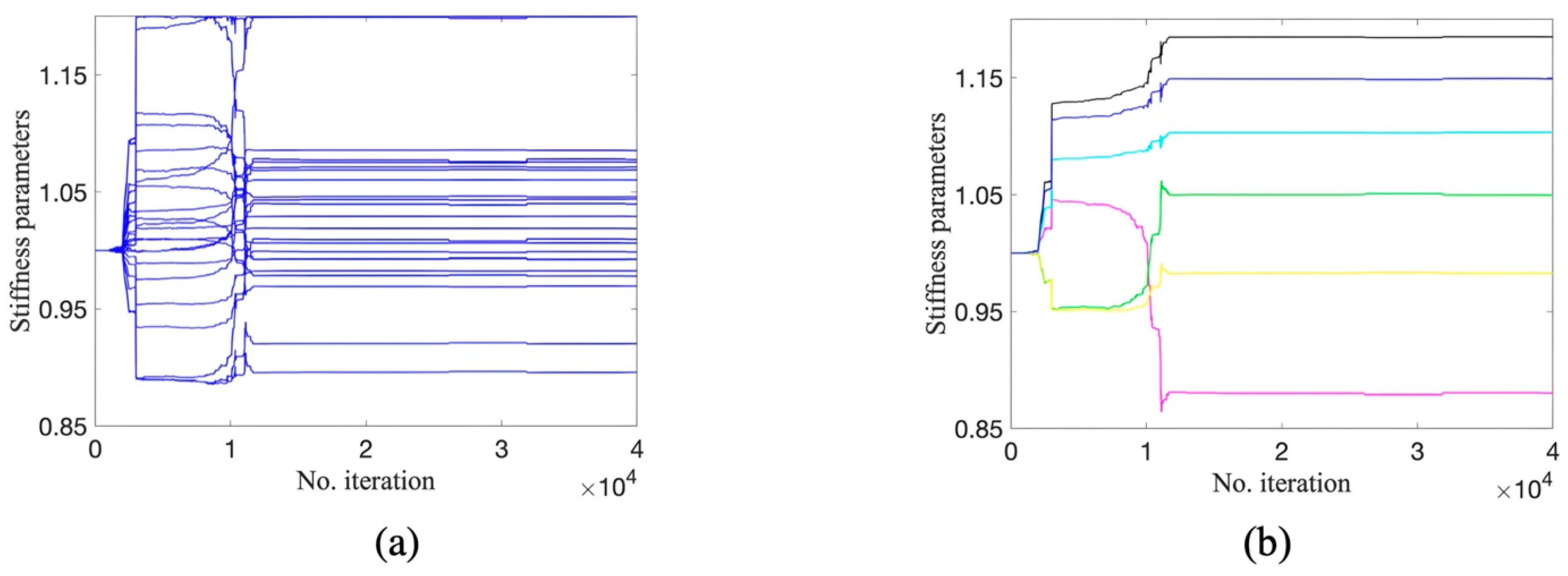
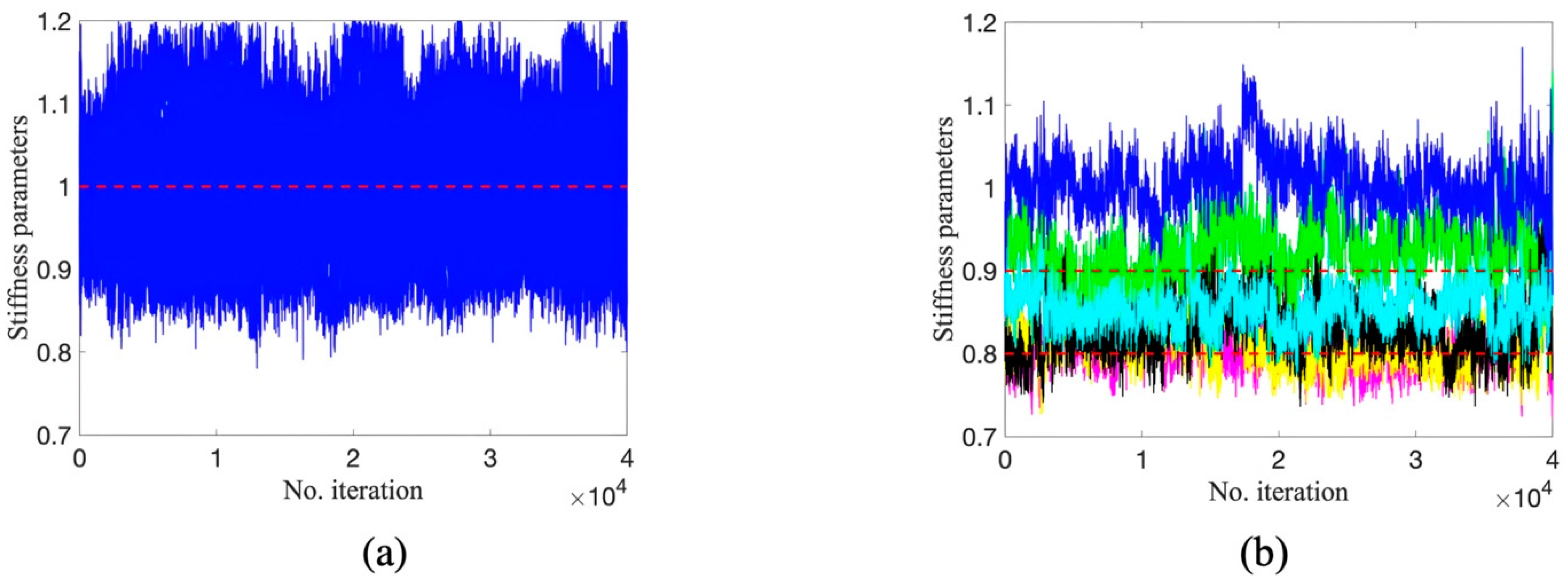
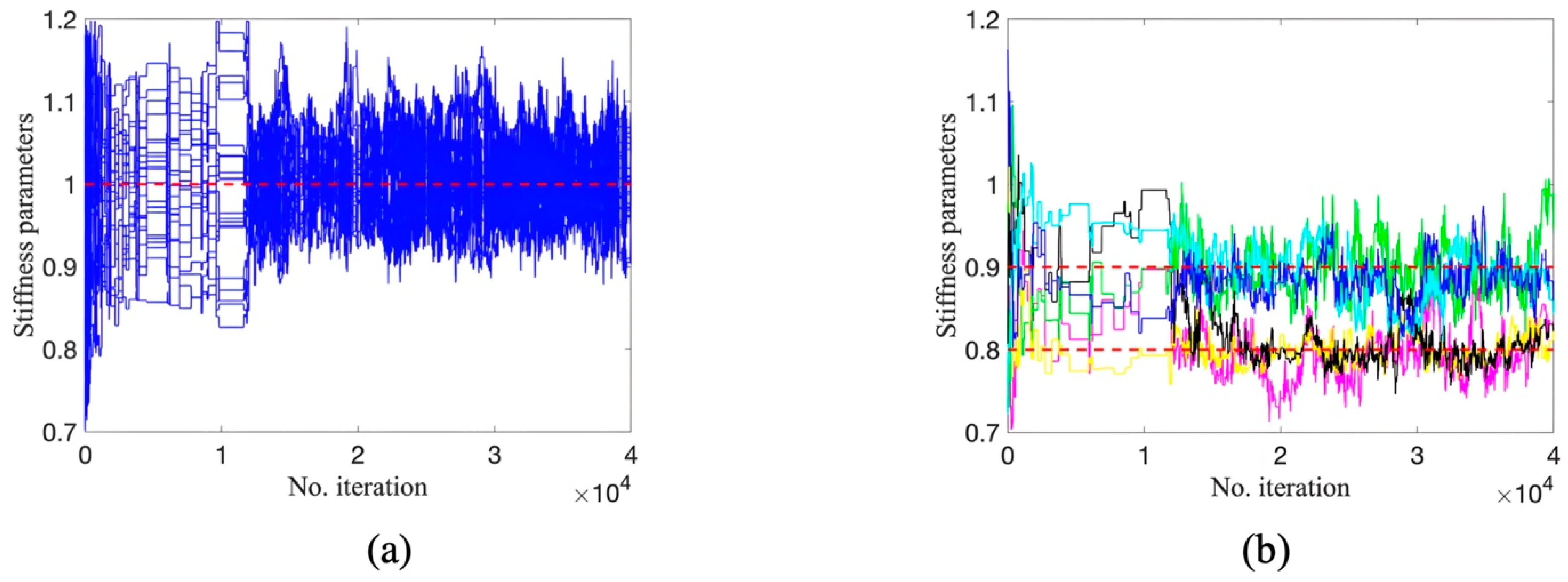
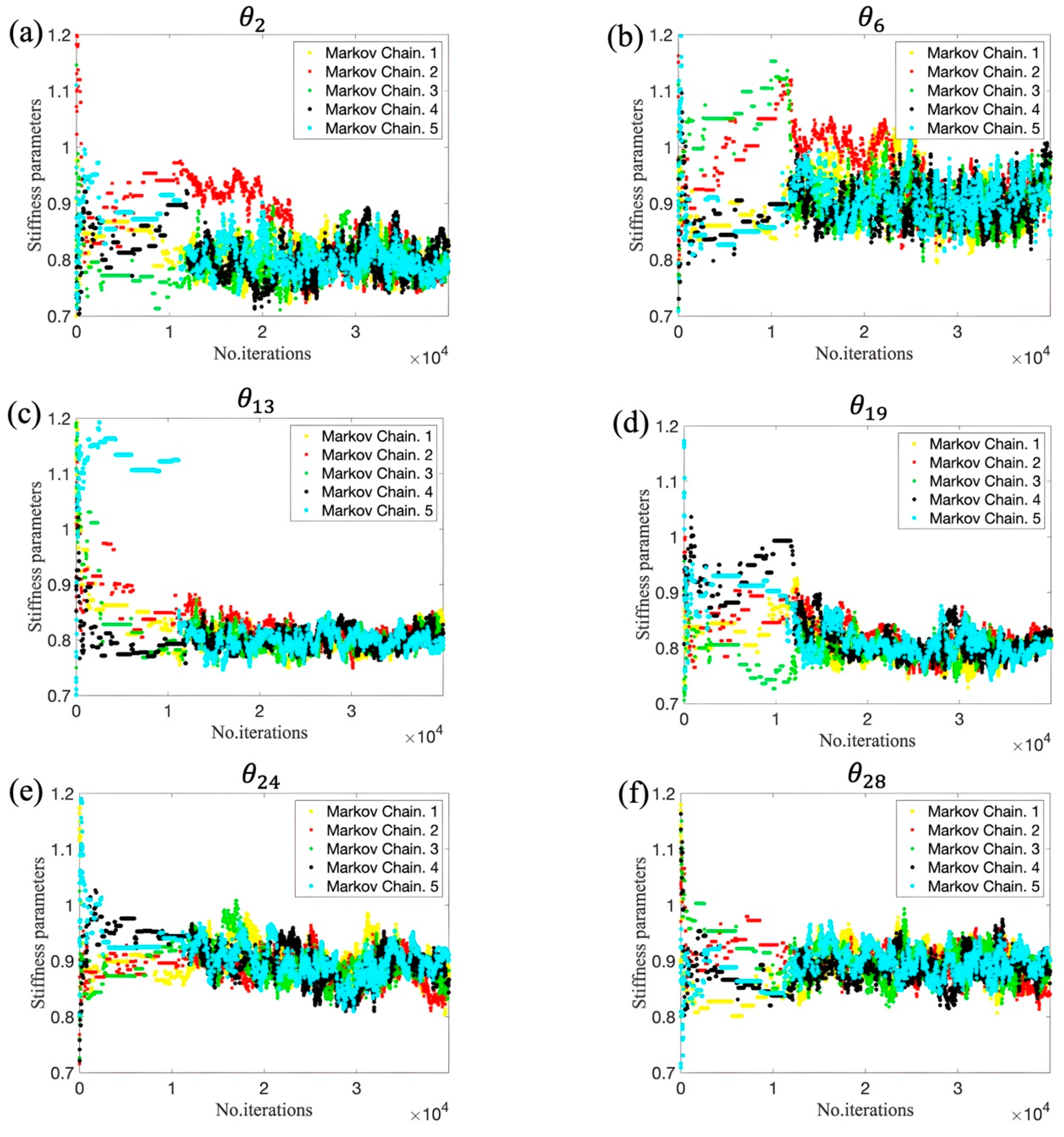

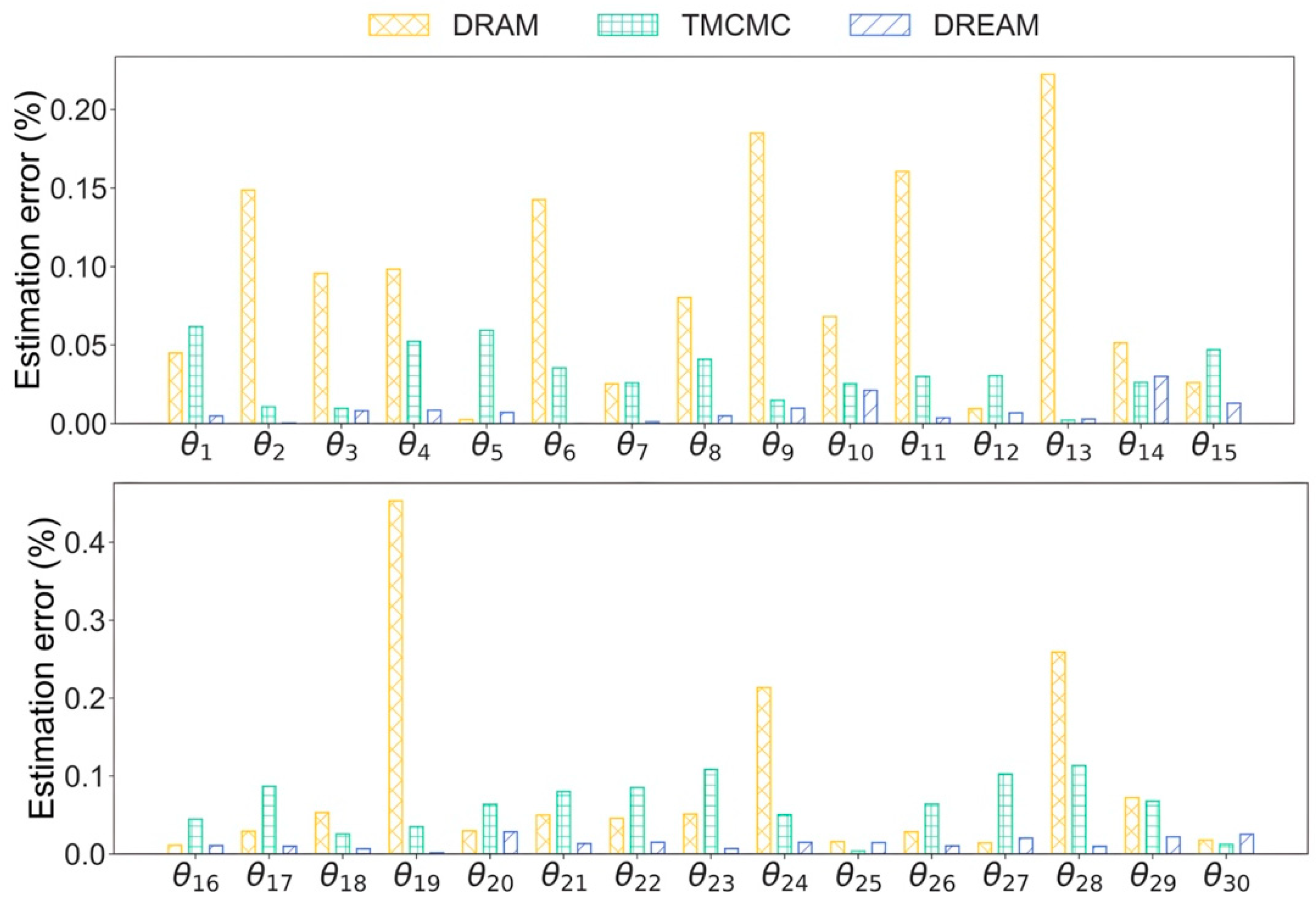

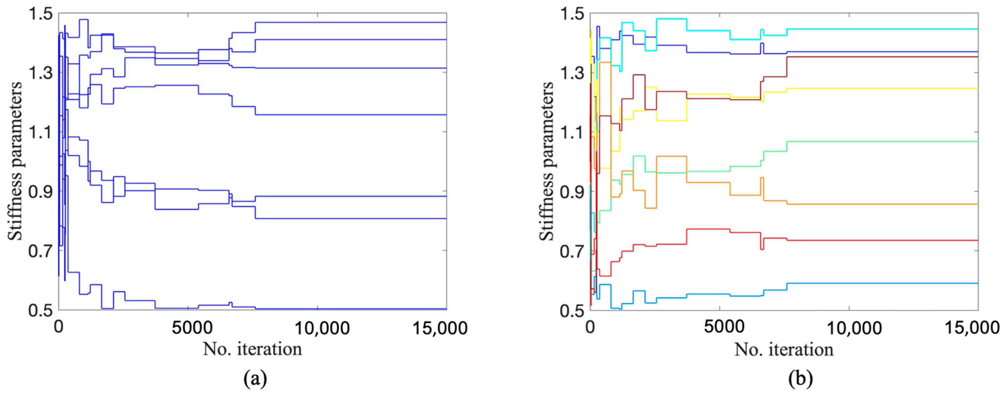
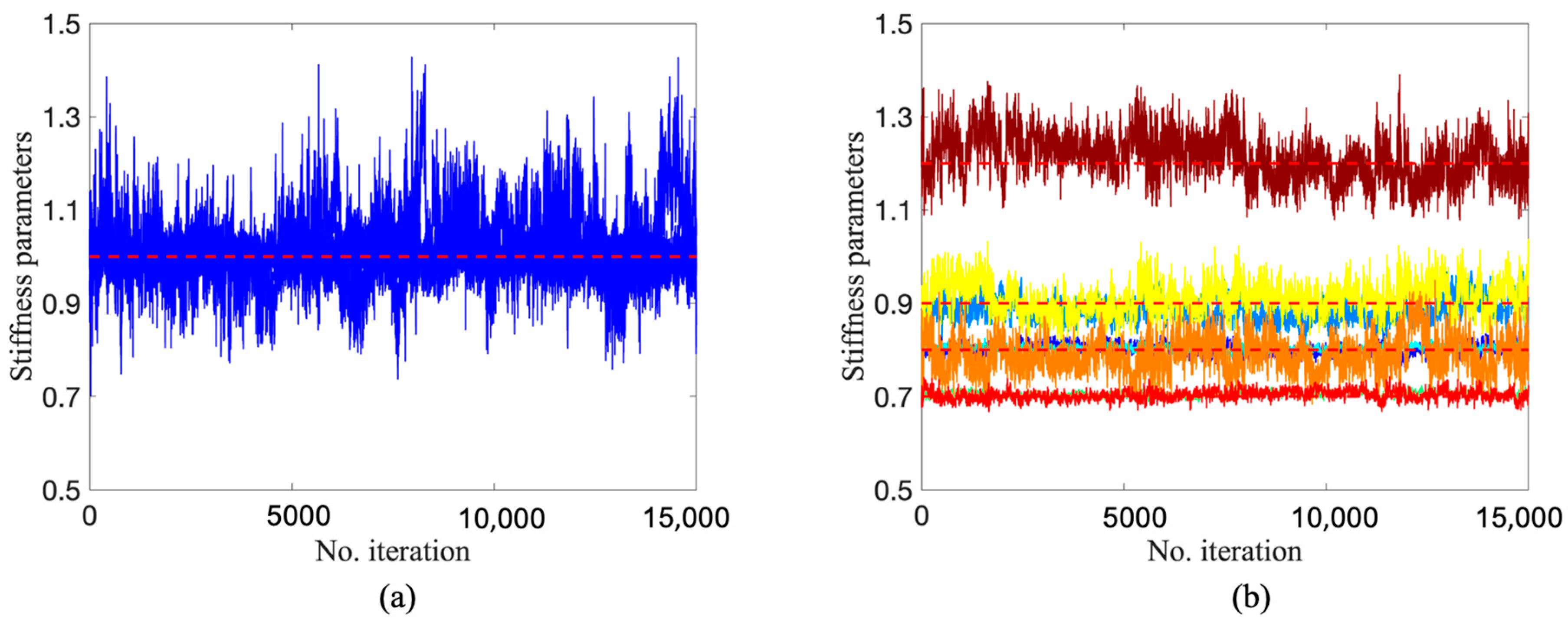
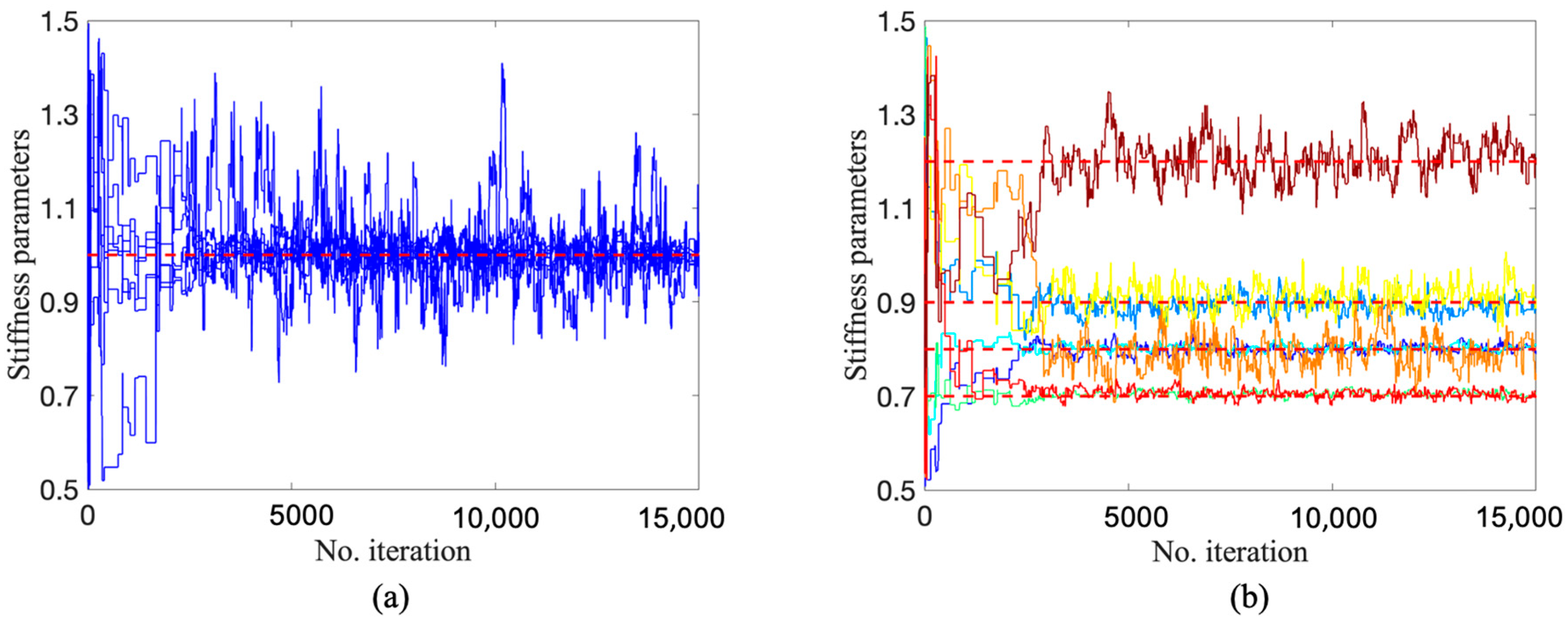
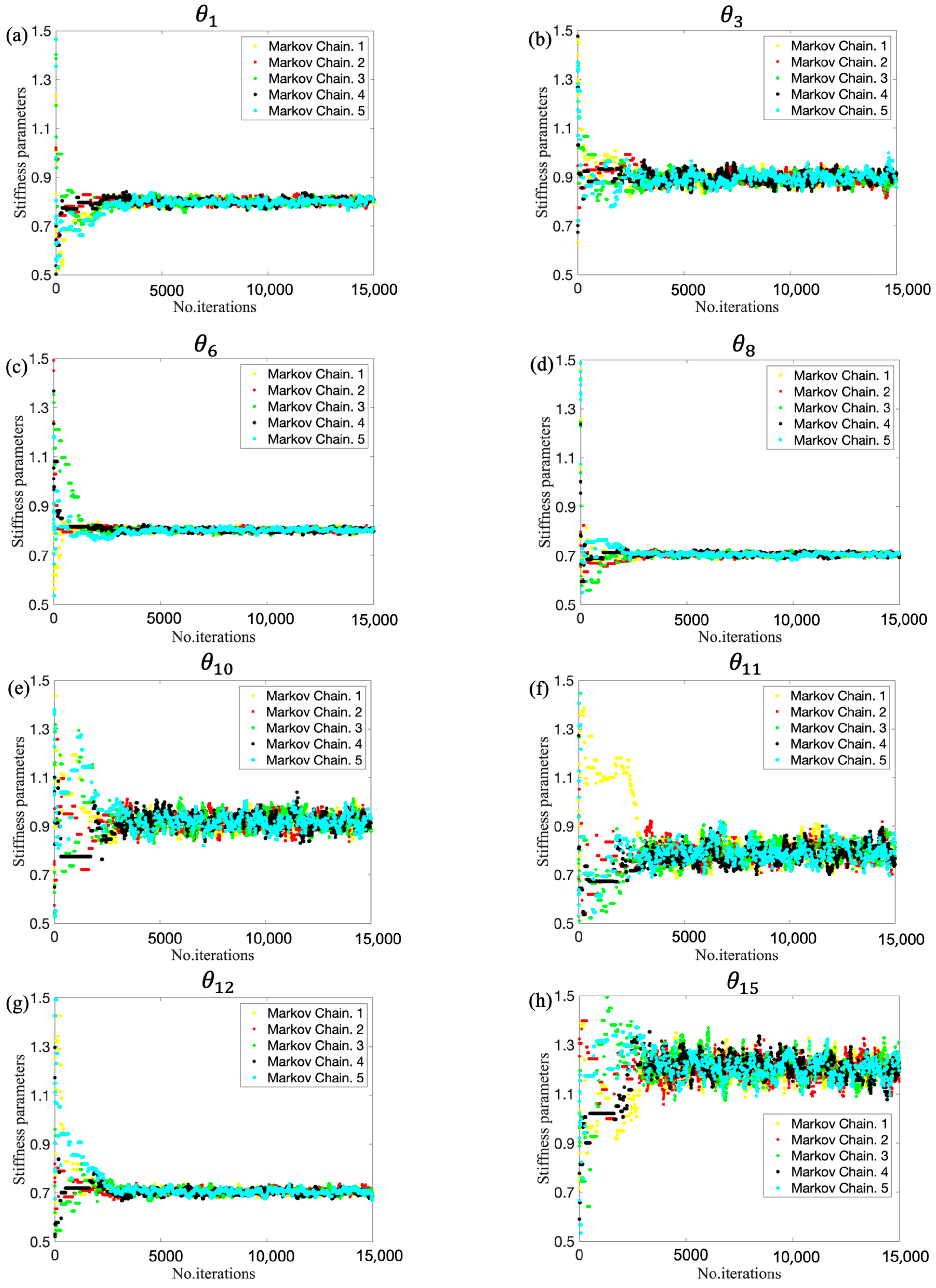
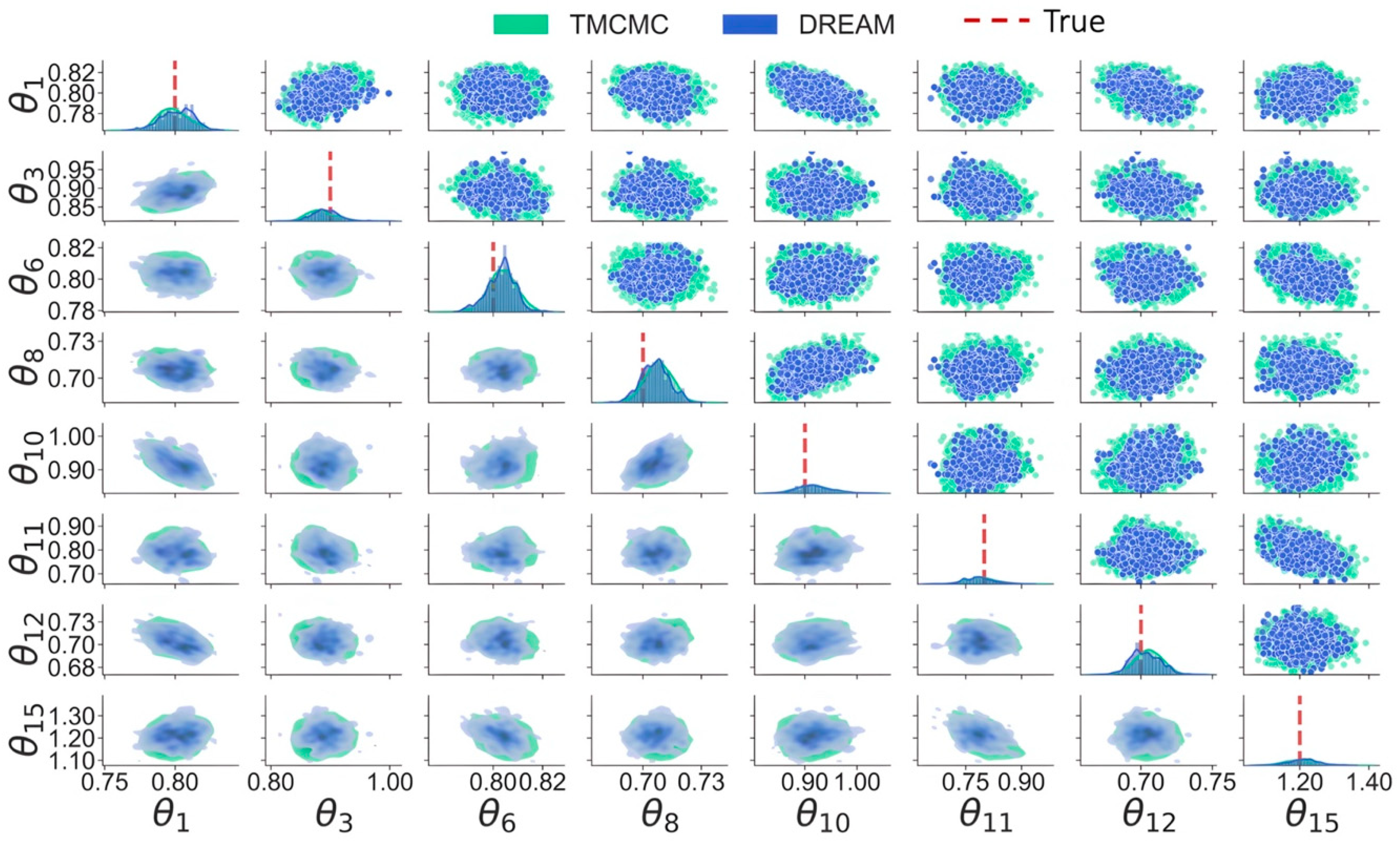
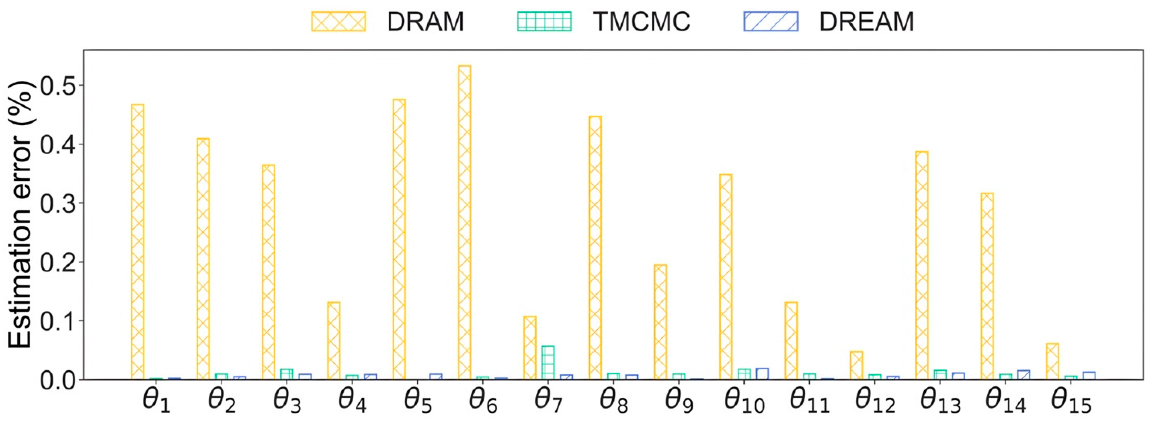
Disclaimer/Publisher’s Note: The statements, opinions and data contained in all publications are solely those of the individual author(s) and contributor(s) and not of MDPI and/or the editor(s). MDPI and/or the editor(s) disclaim responsibility for any injury to people or property resulting from any ideas, methods, instructions or products referred to in the content. |
© 2024 by the authors. Licensee MDPI, Basel, Switzerland. This article is an open access article distributed under the terms and conditions of the Creative Commons Attribution (CC BY) license (https://creativecommons.org/licenses/by/4.0/).