Method of Multi-Label Visual Emotion Recognition Fusing Fore-Background Features

Abstract

This paper proposes a method for multi-label visual emotion recognition that fuses fore-background features to address the following issues that visual-based multi-label emotion recognition often overlooks: the impacts of the background that the person is placed in and the foreground, such as social interactions between different individuals on emotion recognition; the simplification of multi-label recognition tasks into multiple binary classification tasks; and it ignores the global correlations between different emotion labels. First, a fore-background-aware emotion recognition model (FB-ER) is proposed, which is a three-branch multi-feature hybrid fusion network. It efficiently extracts body features by designing a core region unit (CR-Unit) that represents background features as background keywords and extracts depth map information to model social interactions between different individuals as foreground features. These three features are fused at both the feature and decision levels. Second, a multi-label emotion recognition classifier (ML-ERC) is proposed, which captures the relationship between different emotion labels by designing a label co-occurrence probability matrix and cosine similarity matrix, and uses graph convolutional networks to learn correlations between different emotion labels to generate a classifier that considers emotion correlations. Finally, the visual features are combined with the object classifier to enable the multi-label recognition of 26 different emotions. The proposed method was evaluated on the Emotic dataset, and the results show an improvement of 0.732% in the mAP and 0.007 in the Jaccard’s coefficient compared with the state-of-the-art method.

1. Introduction

Emotion recognition has become increasingly integrated into various aspects of daily life and social activities, such as monitoring student learning states [1], enhancing human–computer interaction [2], driver monitoring [3], and lie detection [4].

In visual-based emotion recognition research, facial expressions have traditionally been regarded as the most effective features [5]. The field has seen rapid advancements in facial expression analysis, thus leading to significant progress. However, in real-world scenarios, individuals are often engaged in diverse social activities within varied environments, which makes it challenging to accurately capture facial information due to factors such as head tilts, occlusions, and uneven lighting. Beyond facial expressions, recent studies began to explore additional visual cues. For instance, Aviezer et al. [6] and Martinez [7] conducted psychological experiments in silent environments where participants’ faces were obscured. Their findings revealed that observers could accurately infer emotions through body posture and environmental context, thus suggesting that these factors are also valuable for emotion recognition. Additionally, there has been limited exploration of foreground information, such as social interactions between individuals, which can offer insights into behaviors through features like distance and proximity, thereby enhancing the emotion recognition accuracy.

Most current research on emotion recognition [8,9,10] focuses on the single-label recognition of a few common emotions, such as happiness, sadness, surprise, neutrality, and anger. However, human emotions are inherently complex and multidimensional, and single-label classification falls short of capturing the full spectrum of emotional expression. Emotion datasets [11] encompass 26 fine-grained emotion categories, and multi-label recognition of these categories can provide a more nuanced and comprehensive description of an individual’s emotional state. In multi-label emotion recognition, some studies [12] overlook the relationships between different emotions, often decomposing the task into independent binary classification tasks, which fails to account for the global correlations between all emotion labels and leads to reduced recognition accuracy. Traditional multi-label classification methods, such as ML-KNN [13] and ML-RBF [14], attempt to learn label correlations through kernel functions, loss functions, and association rules. However, these methods are often inefficient and primarily capture local correlations. The self-attention mechanism in Transformer architectures was also employed for modeling label correlations [15,16], but it is more suited for long sequence data and demands substantial computational resources. Graph-based approaches can model label correlations as well, but the construction of the adjacency matrix is crucial. Consequently, developing a multi-label classifier that effectively captures the global correlations of emotions remains a significant challenge.

To address the above issues, this paper proposes a method of multi-label visual emotion recognition that fuses fore-background features. The contributions of this approach are highlighted in three key aspects as follows:

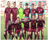
• A fore-background-aware emotion recognition model (FB-ER) is proposed. The background in which the person is placed and the foreground, such as interactions between different individuals, provide beneficial visual cues for emotion recognition, as shown in Figure 1. FB-ER is a three-branch multi-feature hybrid fusion network. It designs a core region unit (CR-Unit) to effectively extract body features, represents background features as background keywords to help the model understand emotion expressions in specific contexts through semantic data, and captures depth map information to better simulate interactions between different individuals as foreground features. These three types of features are fused both at the feature level and the decision level.
• A multi-label emotion recognition classifier model (ML-ERC) is introduced, which utilizes graph convolutional networks (GCNs) to capture label correlations. The nodes in the graph are represented by word-embedding vectors associated with different emotion labels. The edge weights are determined by considering both the label co-occurrence probability matrix, as shown in Figure 2, and the cosine similarity matrix. Information is propagated between nodes by the GCN, which enables the classifier to learn the inter-relational information between emotional labels.
• An end-to-end network architecture that combines FB-ER and ML-ERC was designed for the multi-label recognition of 26 distinct emotions. This architecture demonstrates generalizability across various environments and emotion categories.

The rest of this paper is organized as follows: Section 2 describes the current related work of visual emotion recognition and multi-label emotion classification. Section 3 gives a description of the proposed FB-ER and ML-ERC. Section 4 introduces the experimental designation and verifies the performance of the proposed method. Finally, Section 5 concludes this paper.

2. Related Work

2.1. Visual Emotion Recognition

Significant progress has been made in the study of facial emotions in recent years. These methods have achieved superior performance by developing effective facial feature extraction networks. Siqueira et al. [8] and Karani et al. [10] optimized their CNN models for computational efficiency, which resulted in models with both high computational efficiency and accuracy. Liao et al. [9] enhanced emotion recognition by incorporating facial optical flow information, while Arabian et al. [17] constructed a facial key point grid and utilized GCN for emotion classification. Kim et al. [18] adopted the designs of VGG, Inception-v1, ResNet, and Xception to propose the CVGG-19 architecture for classifying driver emotions, which offers the advantages of high accuracy and low cost. Oh et al. [19] investigated the impact of noise in image data on classification accuracy and proposed a deep learning model to enhance robustness against noise. Khan et al. [20] proposed a novel temporal shifting approach for a frame-wise transformer-based model using multi-head self/cross-attention (MSCA) to reduce the computational cost of emotion recognition. However, these methods focus solely on the facial region and do not consider other visual information beyond the face.

Several studies [11,21,22,23,24] explored the use of visual information beyond facial features. For instance, Mou et al. [21] employed a dual-stream network, where one branch extracted body features and the other extracted environmental features using a k-NN classifier to independently identify arousal and valence from these feature sets. However, due to the simplicity of the feature extraction network, it could not fully capture the necessary features. Additionally, the fusion of the two branches’ outputs occurred at the decision level, without accounting for the influence of environmental features on emotion recognition. Building on this work, Kosti et al. [11], Lee et al. [22], and Zhang et al. [23] concatenated different visual features for emotion classification. Nonetheless, the recognition accuracy varied greatly across different emotions, particularly those that are more difficult to classify. Ilyes et al. [24] proposed a multi-label focal loss function to address the issue of imbalanced emotion categories, which led to improved emotion recognition performance. However, the networks used in these studies exhibited limited feature extraction capabilities, underutilized background features, and relied on the simple concatenation of features without considering their complementarity. Furthermore, foreground information, such as social interactions between individuals, which can provide valuable insights into behavioral characteristics and enhance emotion recognition accuracy, remains underexplored in the current literature.

2.2. Multi-Label Emotion Classification

Multi-label classification methods can be categorized into three strategies: first order, second order, and high order [12]. The first-order strategy decomposes multi-label classification into multiple independent binary classification tasks while neglecting correlations between labels. The second-order strategy considers pairwise label relationships and distinguishes between related and unrelated labels. However, in real-world scenarios, label dependencies often exceed the limitations of second-order correlations. The high-order strategy addresses the associations between multiple labels and the influence of each label on all others, thus providing a more robust framework for modeling label correlations. Traditional high-order methods include ML-KNN [13], ML-RBF [14], BPMLL [25], and MLC-ARM [26]. ML-KNN [13] generates predictions by considering the relevance of local samples, but it fails to capture the global correlations across all labels. ML-RBF [14] employs a kernel function in feature space to account for label dependencies, while BPMLL [25] introduces a ranking loss function to minimize the dissimilarity between labels. However, as data correlations exceed the second-order level, the effectiveness of both ML-RBF and BPMLL becomes constrained. MLC-ARM [26] leverages association rules mined from sample correlations to perform multi-label classification, but its efficiency is hampered by the high computational costs involved.

In recent years, several approaches adapted modified Transformer architectures to learn correlations between different labels. For instance, methods like Q2L [15], ML-Decoder [16], and SAML [27] utilize enhanced Transformer models and the self-attention mechanism to capture inter-label correlations. However, these methods are better suited for capturing correlations in long sequence data and may not perform optimally when modeling label correlations in image data. Additionally, they demand significant computational resources and storage capacity.

In the field of object detection, several studies [28,29,30,31] constructed simple graph structures to represent the relationships between different objects within a single image, where an edge with a value of 0 denotes that two labels are unrelated, and an edge with a value of 1 indicates that they are related. Graph convolutional networks (GCNs) are then employed to learn local correlations across different images. However, these methods fail to account for the varying strengths of label correlations and overlook the global relationships between labels, and the application of GCNs for modeling correlations has seldom been explored in the domain of emotion recognition.

3. Approach

3.1. Fore-Background-Aware Emotion Recognition (FB-ER)

3.1.1. Relationship between Fore-Background and Emotions

Table 1. Example table of correlations between background and emotions.

Index	Description	Approximate Proportion in the Dataset	Original Figure	Emotion (without Background)	Background Heat Map	Background Semantics	Emotion (with Background Information)
No. 1	Completely lacking facial information.	16.7%		-		Beach, water park, sunny, boating, swimming	[“Anticipation”, “Engagement”, “Happiness”, “Pleasure”]
				-		Physics, chemistry lab, working, competing, stressful	[“Fatigue”, “Suffering”]
				-		Ski, mountain, snowy, cold, sunny, far-away horizon	[“Engagement”, “Excitement”]
No. 2	Partial facial information.	45%		Neutral		Ballroom, legislative, beauty salon, socializing, congregating	[“Affection”, “Esteem”, “Happiness”]
				Neutral		Bedroom, enclosed area, cloth, warm, dry	[“Peace”, “Happiness”]
No.3	When facial information is complete, the same facial expression can be observed in different backgrounds.	38.3%		Pain		Hospital, operating, working, stressful, medical activity	[“Pain”, “Sadness”, “Suffering”]
				Pain		Martial gym, competing, sports, exercise, congregating	[“Disquiet”, “Engagement”, “Excitement”]

presents three different scenarios (derived from the Emotic dataset [11] and Google images): First, facial and postural cues are entirely obscured, which makes it impossible to use these features for emotion recognition. In such cases, the background context becomes crucial for inferring emotions. For example, in Scenario 1, individuals are shown sunbathing; although their faces are not visible, elements like clear water and a bright sky suggest a happy mood. Second, as illustrated in Scenario 2, faces and postures are partially covered. In these instances, emotions are often classified as neutral, which implies neither happiness nor sadness. However, by considering the background, alternative interpretations may arise. For instance, in a wedding setting, more fitting emotions could include affection, esteem, or happiness. Third, when facial expressions are fully visible, as shown in Scenario 3, the same expression can convey different emotions depending on the background context. For example, both expressions in Scenario 3 were initially classified as pain. Yet, with background consideration, one image set in a hospital and the other in a sports stadium, the latter scenario might more accurately reflect emotions such as disquiet, engagement, or excitement.

Next, the relationships between the foreground and emotions are examined. In this context, the foreground refers to the interactions between individuals within the image. These interactions can be divided into two scenarios, as depicted in

Table 2. Example table of correlations between foreground and emotions.

Index	Description	Approximate Proportion in the Dataset	Original Figure	Depth Map	Emotions of Character A	Emotions of Character B
No. 1	Interaction occurs when individuals share a common identity or mutual familiarity.	10.4%			[“Affection”, “Happiness”]	[“Affection”, “Happiness”]
					[“Confidence”, “Engagement”]	[“Confidence”, “Engagement”]
No. 2	Having different identities or being unfamiliar with one another.	19.6%			[“Engagement”]	[“Anticipation”, “Esteem”]
					[“Anticipation”, “Confidence”, “Excitement”]	[“Peace”, “Engagement”]

(using images from the Emotic dataset [11] and Google): First, when individuals share a common identity or are familiar with one another, their emotional tendencies often converge, as illustrated in Scenario 1. Second, when individuals possess different identities or are unfamiliar with each other, their emotional tendencies may diverge, as shown in Scenario 2. This suggests that emotions can spread rapidly through social interactions, and an individual’s emotional state is significantly influenced by their interactions with others.

3.1.2. Emotion Recognition Fusing Fore-Background Features

FB-ER consists of three sub-network branches, as depicted in Figure 3. The first branch is dedicated to the human body, where it extracts essential cues, such as facial expressions and body postures. To achieve this, ResNet18 [32] is utilized as the backbone network for feature extraction. Transfer learning is employed to fine-tune the pre-trained model developed by Krizhevsky et al. [33]. Following the extraction of the body features, a CR-Unit is introduced to emphasize regions that contribute the most to emotion recognition. The structure of the CR-Unit is presented in Figure 4, with its mathematical formulation detailed in Equations (1)–(3):

$$f\left(F_{body},nu{m}_1\right)=BatchNorm\left(Linea{r}_1\left(F_{body},nu{m}_1\right)\right)$$

(1)

$$Core\_weights=Adaptive\left[\sigma \left(Linea{r}_2\left(nu{m}_1,nu{m}_2\right)\right)\right]$$

(2)

$$F_{core}=\mathrm{diag}\left[dot\left(F_{body},Attention\_weights\right)\right]$$

(3)

In Equation (1), $F_{body}$ represents the body features, which are mapped to length $nu{m}_1$ through $Linea{r}_1$, followed by $BatchNorm$. In Equation (2), the features are mapped from length $nu{m}_1$ to length $nu{m}_2$ by $Linea{r}_2$, and then $Core\_weights$ of the same length as $F_{body}$ is obtained using $Sigmoid$ and $Adaptive$. In Equation (3), $dot$ denotes the dot product operation, and $diag$ represents the extraction of diagonal elements, thus ultimately yielding $F_{core}$. $F_{core}$ focuses more on the regions of $F_{body}$ that are beneficial for emotion classification, thus effectively enhancing the model’s ability to recognize the important parts of the $F_{body}$.

The second sub-network branch was designed for background feature extraction, which provides useful information for understanding the emotions of individuals in the image. The background can be considered as a set of keywords associated with objects and ongoing activities within a scene. To evaluate the scene comprehension, the Places365 model [34] was utilized. The results presented in

Table 3. Background semantic recognition.

Original Figure	Heat Map	Recognition Results
		Outdoors, cliff, natural, sunny, climbing, rugged scene, far away horizon
		Indoors, office, working, studying, enclosed area, no horizon

exhibit two different scenes: outdoors and indoors. For the outdoor scene, the recognition keywords include “outdoor”, “cliff”, “climbing”, and “sunny”. For the indoor scene, the keywords include “indoor”, “office”, “working”, and “closed area”. ResNet18 was also employed for extracting background features. Transfer learning techniques were used to fine-tune the pre-trained weights of the Places365 model in this study.

The third sub-network branch was designed for foreground feature extraction, which primarily includes the interactions between different individuals. These interactions are valuable for emotion evaluation. This study adopted a method based on depth map extraction to simulate the interaction and proximity between different individuals. The steps are organized as follows:

Step 1—Data preprocessing: all images in the dataset are normalized to RGB three channels.

Step 2—Depth map extraction: MegaDepth [35] is a powerful tool for depth map extraction that was designed to generate depth information from single-view images using advanced stereo matching techniques. Its pre-trained models exhibit a high accuracy and reliability, which enables precise depth map extraction across diverse scenes, lighting conditions, and viewpoints. Therefore, we utilized the MegaDepth pre-trained model to obtain depth maps from the original images.

Step 3—Color rendering: color rendering is applied to the acquired depth map to enhance the visual effect, as illustrated in Figure 5.

Step 4—Depth matrix calculation: The depth matrix information D of the depth map is calculated using Equation (4) presented below:

$$D=\left[\left(\begin{array}{cccc}D\left(1,1\right)& D\left(1,2\right)& ....& D\left(1,N\right)\\ D\left(2,1\right)& D\left(2,2\right)& ....& D\left(2,N\right)\\ ....& ....& ....& ....\\ D\left(M,1\right)& D\left(M,2\right)& ....& D\left(M,N\right)\end{array}\right)\right]$$

(4)

where D represents a matrix of dimensions $M\times N$, and $D\left(i,j\right)$ denotes the depth value corresponding to column j in row i within the depth map. The third sub-network branch comprises three convolutional layers, three pooling layers, and three fully connected layers, which collectively extracts distinctive features from the depth map.

By extracting the aforementioned features and performing shape adjustment, the following features are obtained: core feature $F_{core}$, background feature $F_{back}$, foreground feature $F_{fore}$, and fusion feature $F_{mix}$:

$$\left\{\begin{array}{c}{F}_{core}\to batchsize\times d_1\hfill \\ F_{back}\to batchsize\times d_2\hfill \\ F_{fore}\to batchsize\times d_3\hfill \end{array}\right.$$

(5)

$$\left\{\begin{array}{c}{F}_{mix}=F_{core}\left|\right|F_{back}\left|\right|F_{fore}\hfill \\ F_{mix}\to batchsize\times \left(d_1+d_2+d_3\right)\hfill \end{array}\right.$$

(6)

where $d_i$ represents the vector length and $\left|\right|$ denotes the concatenation operation. Subsequently, $F_{core}$, $F_{back}$, and $F_{mix}$ are combined with the multi-label object classifier to perform emotion recognition for 26 different types of emotions. The optimal weights of the three emotion recognition results are obtained through training, and different weights are assigned to represent the relative importances of $F_{core}$, $F_{back}$, and $F_{mix}$.

3.2. Multi-Label Emotion Recognition Classifier (ML-ERC)

3.2.1. The Design of the Label Co-Occurrence Probability Matrix

$G=\left\{N,E\right\}$ represents a global label correlation graph structure, where N represents all nodes and E represents all edges within the graph, as illustrated in Equations (7) and (8):

$$\left\{\begin{array}{c}N=\left\{n_1,n_2,n_3,\dots \dots ,n_m\right\}\hfill \\ n_{k\in \left[1,m\right]}=R_k^{\omega }\Rightarrow N={\mathbb{R}}^{m\times \omega }\hfill \\ N={\mathbb{R}}^{m\times \omega }=\left\{R_1^{\omega },R_2^{\omega },R_3^{\omega },\dots \dots ,R_m^{\omega }\right\}\hfill \end{array}\right.$$

(7)

$$\left\{\begin{array}{c}E=\left\{e_{ij}{|}_{i,j\in \mathsf{\Omega }}\right\}\hfill \\ {\left(e_{ij}\right)}_{i,j\in \mathsf{\Omega }}={\left({\theta }_{ij}\right)}_{i,j\in \mathsf{\Omega }}\hfill \end{array}\right.$$

(8)

In Equation (7), each graph node, as denoted by $n_k$, corresponds to an emotion type, where $k\in \left[1,m\right]$, with m representing the number of emotion categories. Each node is represented by a word-embedding vector $R_k^{\omega }$ with a length of $\omega$ using Word2Vec and GloVe. Consequently, all the nodes in the graph structure can be represented as ${\mathbb{R}}^{m\times \omega }$. In Equation (8), $e_{ij}$ represents the edge between node i and node j, Ω represents the set of all edges in the graph structure, and ${\theta }_{ij}$ denotes the weight of the edge between node i and node j. A larger value of ${\theta }_{ij}$ indicates a stronger association between nodes i and j.

In this study, the correlation between different emotions was determined by analyzing the co-occurrence patterns of labels. A represents the label co-occurrence probability matrix, which can be constructed as follows:

Step 1: Compute the co-occurrence count $C{\left(i,j\right)}_{i,j\in \left[1,m\right]}$ of each pair of emotion labels i and j statistically from the dataset.

Step 2: Compute the conditional probability $P\left(i|j\right)$ for each pair of emotion labels in Equation (9):

$$P\left(i|j\right)={\displaystyle \frac{P\left(ij\right)}{P\left(j\right)}}={\displaystyle \frac{C{\left(i,j\right)}_{i,j\in \left[1,m\right]}}{C{\left(j\right)}_{j\in \left[1,m\right]}}}$$

(9)

$C{\left(j\right)}_{j\in \left[1,m\right]}$ represents the frequency of occurrence of emotion label j, while $C{\left(i,j\right)}_{i,j\in \left[1,m\right]}$ represents the frequency of co-occurrence of emotion labels i and j.

Step 3: Construct the conditional probability matrix P:

$$P=\left[\begin{array}{cccc}1& P\left(2|1\right)& \dots & P\left(m|1\right)\\ P\left(1|2\right)& 1& \dots & P\left(m|2\right)\\ \dots & \dots & \dots & \dots \\ P\left(1|m\right)& P\left(2|m\right)& \dots & 1\end{array}\right]$$

(10)

Step 4: According to Equation (11), a judgment is made on whether there is a correlation between different emotional labels. $\tau$ represents the empirical threshold, which indicates the degree of correlation between i and j. Values lower than $\tau$ indicate a weaker correlation and should be ignored. After many experimental verifications, $\tau$ was set to 0.2.

$$\widehat{P}=\left\{\begin{array}{c}0,ifP\left(j|i\right)<\tau \hfill \\ 1,ifP\left(j|i\right)\ge \tau \hfill \end{array}\right.$$

(11)

Step 5: The normalization operation in Equation (12) is used to balance the connection weights between different nodes. The parameter $\lambda$ was set to $1\times {10}^{-6}$, which was used to prevent the denominator from being zero.

$${\tilde{P}}_{ij}=\left\{\begin{array}{c}{\displaystyle \frac{{\widehat{P}}_{ij}}{\lambda +{\sum }_{i=1}^m{\widehat{P}}_{ij}}},i\ne j\hfill \\ 1,i=j\hfill \end{array}\right.$$

(12)

Step 6: To ensure more balanced and stable feature updates in the GCN and improve the model’s performance, further normalization of ${\tilde{P}}_{ij}$ is applied using Equations (13)–(15) based on the normalized Laplacian matrix principle. $D_{ij}$ represents the degree matrix, and A represents the label co-occurrence probability matrix.

$$D_{ij}=\left\{\begin{array}{c}{\sum }_{j=1}^m{\tilde{P}}_{ij},i=j\hfill \\ 0,i\ne j\hfill \end{array}\right.$$

(13)

$${\tilde{D}}_{ij}=D_{ij}^{-{\displaystyle \frac{1}{2}}}$$

(14)

$$A=\left\{\begin{array}{c}{\tilde{D}}_{ij}\tilde{P}{\tilde{D}}_{ij},i\ne j\hfill \\ 1,i=j\hfill \end{array}\right.$$

(15)

3.2.2. The Design of the Cosine Similarity Matrix

Continuous convolution in GCNs reduces the similarity of node representations in the original feature space, as illustrated in Figure 6a,b. Figure 6a shows the Isomap [36] dimensionality reduction plot of the initial node semantic features ${\mathbb{R}}^{m\times \omega }$, where semantically similar emotions are closely positioned, such as “Excitement, Happiness, Pleasure”, “Anger, Annoyance, Aversion”, and “Suffering, Pain”. Figure 6b shows the Isomap dimensionality reduction plot of the node semantic features ${\mathbb{R}}^{m\times \omega }$ after two layers of convolution, where the similarity of node semantic features is disrupted, with semantically similar emotions positioned far apart and dissimilar emotions positioned close together.

To prevent consecutive convolution operations from disrupting the similarity of node features, a cosine similarity matrix C is introduced to ensure that the semantic similarity of nodes remains unchanged after each convolution. The construction is organized as follows:

Step 1: Obtain the initial cosine similarity matrix $C_{ij}$ according to Equation (16):

$$C_{ij}={\displaystyle \frac{R_i^{\omega }·R_j^{\omega }}{\left|\right|R_i^{\omega }\left|\right|\left|\right|R_j^{\omega }\left|\right|}}$$

(16)

where $\left|\right|\dots \left|\right|$ represents the $L_2$ norm.

Step 2: To ensure that similarity values between different emotion categories are on the same scale, eliminate dimensional discrepancies, and reduce the impact of extreme values, normalize $C_{ij}$ by the Z-score to obtain the cosine similarity matrix C. Figure 7b illustrates the resulting C using ${\mathbb{R}}^{m\times \omega }{|}_{Glove}$ as an example.

3.2.3. Label Correlation Emotion Classifier

Under the dual constraints of co-occurrence probability matrix A and cosine similarity matrix C, the GCN aggregates each label node to update its representation, thus effectively capturing inter-label association information. This approach results in an object classifier capable of learning the correlations between emotion labels.

The input to the GCN includes the word-embedding vectors of all nodes ${\mathbb{R}}^{m\times \omega }$, the label co-occurrence probability matrix A, and the label cosine similarity matrix C. By stacking multiple GCN layers, the network is able to learn and model the complex relationships between nodes, as described in Equation (17):

$${\left({\mathbb{R}}^{m\times \omega }\right)}^{l+1}=\sigma \left({\displaystyle \frac{A{\left({\mathbb{R}}^{m\times \omega }\right)}^l{W}_a^l+C{\left({\mathbb{R}}^{m\times \omega }\right)}^l{W}_c^l}{2}}\right)$$

(17)

l represents the l-th layer of the GCN, while $W_a^l$ and $W_c^l$ are the weight matrices that need to be learned. Each layer takes the input from the previous layer and updates the output according to Equation (17).

The final output of each GCN node is a classifier $h_i$ for the corresponding emotion label, as shown in Equation (18):

$$H={\left\{h_i\right\}}_{i=1}^m={\left({\mathbb{R}}^{m\times \omega }\right)}^L,h_i={\left(R_i^{\omega }\right)}^L$$

(18)

The final emotion prediction score is denoted as $\widehat{y}$, as shown in Equation (19):

$$\left\{\begin{array}{c}\widehat{y}={\eta }_1{F}_{core}{H}^T+{\eta }_2{F}_{back}{H}^T+{\eta }_3{F}_{mix}{H}^T\hfill \\ {\eta }_1+{\eta }_2+{\eta }_3=1\hfill \end{array}\right.$$

(19)

where $F_{core}$, $F_{back}$, and $F_{mix}$ denote the features of the body’s core region, background features, and fused features mentioned earlier, respectively. ${\eta }_i$ represents the trainable coefficient, which indicates the relative importances of $F_{core}$, $F_{back}$, and $F_{mix}$. Initially, the values were assigned as ${\eta }_1=0.333$, ${\eta }_2=0.333$, and ${\eta }_3=0.333$. After several epochs of iteration, the optimal predictive performance of the model was achieved when ${\eta }_1=0.3$, ${\eta }_2=0.2$, and ${\eta }_3=0.5$. $H^T$ denotes the transpose operation of H. Both feature-level fusion and decision-level fusion are employed for the final emotion identification.

4. Experimental Section

4.1. Dataset

The Emotic dataset [11] was employed in the experiment due to its comprehensive annotations across 26 different emotion categories. The images in this dataset feature complex backgrounds that encompass diverse environments, times, locations, camera viewpoints, and lighting conditions. Therefore, the proposed method demonstrates generalizability across different environments and emotion categories. These inherent characteristics provide the dataset with remarkable diversity, which made the experimental task significantly more challenging.

The dataset was divided into four subsets: Ade20k, Emodb-small, Framesdb, and Mscoco. The sample distribution within the dataset was imbalanced, with varying quantities for each type of emotion. Positive emotions were more prevalent, while negative emotions were less represented. During the experiments, the dataset was partitioned into training, validation, and test sets, as shown in

Table 4. Dataset statistics.

Data Distribution	-	Quantity
Sub-dataset distribution	Ade20k	432
	Emodb-small	1374
	Framesdb	4869
	Mscoco	16,510
Sample distribution	Affection	1063
	Anger	209
	Annoyance	368
	Anticipation	5335
	Aversion	168
	Confidence	4059
	Disapproval	659
	Disconnection	325
	Disquietment	1462
	Doubt/Confusion	479
	Embarrassment	152
	Engagement	12,814
	Esteem	851
	Excitment	4394
	Fatigue	538
	Fear	177
	Happiness	5630
	Pain	188
	Peace	1691
	Pleasure	2103
	Sadness	405
	Sensitivity	360
	Suffering	260
	Surprise	417
	Sympathy	718
	Yearning	668
Data partition	Training	23,265
	Validation	3314
	Test	7202

.

4.2. Loss Function and Evaluation Metrics

Due to the imbalanced sample distribution in the Emotic dataset, we utilized the multi-label focal loss [24] as the loss function in this study, which is expressed as Equation (20):

$$MF{L}_{\alpha ,\gamma }\left(y,\widehat{y}\right)=-\sum _{i=1}^{26}[\alpha {\left(1-{\widehat{y}}_i\right)}^{\gamma }{y}_{i}log\left({\widehat{y}}_i\right)+\left(1-\alpha \right){\left({\widehat{y}}_i\right)}^{\gamma }\left(1-y_i\right)log\left(1-{\widehat{y}}_i\right)]$$

(20)

where ${\widehat{y}}_i$ represents the predicted label of the i-th category, $y_i$ represents the true label of the i-th category, and $\alpha$ and $\gamma$ are two hyperparameters. The balance factor $\alpha$ effectively balances the overall contributions of the positive and negative samples, while the focusing parameter $\gamma$ adjusts the weights of the easy and hard samples. The optimal recognition performance of the model was achieved when $\alpha =0.5$ and $\gamma =0.3$ through multiple experiments.

The evaluation metrics were the average precision (AP), mean average precision (mAP), Jaccard coefficient (JC), total parameters (Params), and floating point operations (FLOPs). mAP and JC are defined as follows in Equations (21) and (22):

$$mAP={\displaystyle \frac{{\sum }_{i=1}^{m}A{P}_i}{m}}$$

(21)

$$JC={\displaystyle \frac{\left|y\cap \widehat{y}\right|}{\left|y\cup \widehat{y}\right|}}$$

(22)

The AP is an approximation of the area under the precision–recall curve and assesses the model’s average precision at all recall levels. In Equation (21), i represents different emotion categories, and m represents the total number of emotion categories. mAP is a global metric that evaluates the average performance of the model across all categories. In Equation (22), y represents the true labels, $\widehat{y}$ represents the predicted results, and the JC measures the degree of overlap between the predicted results and the true labels. The model’s predictive performance value ranged between 0 and 1, with a higher value indicating better performance.

4.3. Comparative Experiments

The methods proposed in this paper were compared with several existing approaches, namely, ML-KNN [13], ML-RBF [14], Kosti et al. [11], Lee et al. [22], Zhang et al. [23], ML-GCN [28], ESRs [8], Ilyes et al. [24], Q2L [15], LGLM [29], RCL-Net [9], ML-Decoder [17], SAML [27], FLNet [30], BHARAT [10], and LFPLM [17]. The emotion precision of these methods is shown in

Table A1. Category precisions of different models.

Emotions	Average Precision (%)
	Kosti [11]	Lee [22]	Zhang [23]	Ilyes [24]	ESRs [8]	RCL-Net [9]	BHARAT [10]	LFPLM [17]	Ours
Affection	27.851	18.960	46.895	31.926	27.426	27.887	32.940	30.098	34.056
Anger	9.489	6.251	10.876	13.942	8.973	16.827	14.318	12.449	17.688
Annoyance	14.062	8.713	11.271	17.424	14.897	10.115	18.386	17.344	22.384
Anticipation	58.641	50.019	62.648	57.735	59.022	60.102	94.231	94.848	95.201
Aversion	7.477	4.975	5.935	8.192	7.305	3.236	12.913	15.767	19.033
Confidence	78.352	58.476	72.497	75.295	76.188	60.213	77.074	68.449	76.165
Disapproval	14.971	7.408	11.283	14.884	14.969	9.988	14.908	17.008	19.566
Disconnection	21.320	19.200	26.916	28.323	21.698	20.064	30.400	32.162	40.001
Disquiet	16.886	13.841	16.942	19.724	18.552	10.005	18.640	20.285	22.863
Doubt/Confusion	29.627	14.802	18.684	23.115	29.264	20.012	24.765	18.835	21.362
Embarrassment	3.182	3.445	2.010	2.847	5.616	5.553	9.827	10.769	11.255
Engagement	87.531	77.633	88.562	85.838	87.611	80.125	99.510	95.060	97.264
Esteem	17.730	13.066	13.338	16.725	17.829	17.893	26.357	28.092	35.431
Excitement	77.157	58.581	71.891	70.436	79.252	62.316	76.246	66.464	79.018
Fatigue	9.700	6.432	13.263	14.434	9.783	9.942	12.089	13.114	13.463
Fear	14.144	4.732	5.687	8.277	14.248	3.883	14.098	11.934	13.527
Happiness	58.261	56.927	73.265	76.626	59.335	56.833	73.658	75.718	72.648
Pain	8.942	7.960	3.527	9.385	8.666	8.001	14.887	12.365	19.556
Peace	21.588	18.071	32.852	24.318	21.968	22.013	30.914	26.157	32.432
Pleasure	45.462	35.300	57.466	46.893	46.380	39.976	50.756	41.873	52.363
Sadness	19.661	9.588	10.388	23.946	19.524	13.273	22.279	13.355	28.674
Sensitivity	9.280	4.414	4.976	6.286	9.331	3.439	9.344	9.609	9.721
Suffering	18.839	8.372	4.477	26.245	19.527	10.018	21.585	12.628	18.568
Surprise	18.810	10.265	9.024	10.110	18.224	10.258	19.050	17.025	26.387
Sympathy	14.711	10.781	17.536	13.984	13.422	10.523	30.965	30.423	34.255
Yearning	8.343	7.046	10.559	9.717	8.652	7.100	22.157	19.486	22.524
mAP(%)	27.384	20.587	27.030	28.332	27.602	23.061	33.549	31.205	35.977

in Appendix A. The comparison results of the mAP and JC are shown in

Table 5. The mAP and JC of different methods. The bold parts represent the optimal values of the model.

Experiment	mAP (%)	JC	Params (M)	FLOPs (G)
ML-KNN [13] (2007)	32.531	0.400	11.704	10.240
ML-RBF [14] (2011)	23.665	0.399	11.926	10.470
Kosti et al. [11] (2019)	27.384	0.349	44.820	7.803
Lee et al. [22] (2019)	20.587	0.269	16.010	9.207
Zhang et al. [23] (2019)	27.030	0.353	30.582	9.553
ML-GCN [28] (2019)	35.245	0.372	46.960	8.410
ESRs [8] (2020)	27.602	0.355	20.330	9.436
Ilyes et al. [24] (2020)	28.332	0.360	39.400	23.400
Q2L [15] (2021)	34.243	0.416	18.013	8.310
LGLM [29] (2022)	29.494	0.275	20.956	8.414
RCL-Net [9] (2023)	23.061	0.295	54.881	9.410
ML-Decoder [16] (2023)	35.204	0.386	35.024	8.511
SAML [27] (2023)	34.490	0.443	33.614	6.660
FLNet [30] (2023)	29.026	0.365	35.750	7.440
BHARAT [10] (2024)	33.549	0.418	37.769	3.216
LFPLM [17] (2024)	31.205	0.402	12.810	4.326
Ours	35.977	0.450	33.500	5.500

and Figure 8. The results indicate that the methods proposed in this paper achieved the best performance in terms of the mAP and JC, with the mAP exceeding the state-of-the-art by 0.732% and the JC by 0.007, and there was no significant increase in the model total parameters and FLOPs.

4.4. Ablation Experiments

4.4.1. Ablation Experiments of FB-ER and ML-ERC

To validate the effectiveness of FB-ER and ML-ERC, three ablation experiments were conducted. In the first experiment, only FB-ER was retained, without the inclusion of ML-ERC. In the second experiment, only ML-ERC was used and FB-ER was omitted. In the third experiment, both FB-ER and ML-ERC were utilized. The results of these experiments are presented in Figure 9. The findings demonstrate that both components of the proposed method contributed significantly to its overall effectiveness.

4.4.2. Ablation Experiments of FB-ER

Four experiments were conducted using different combinations of branches while keeping all other experimental parameters constant. In the first experiment, only the body information was utilized. The second experiment combined the body information with the background information. The third experiment integrated the body information with the foreground information, and the fourth experiment fused the body information with both the foreground and background information. The resulting average precision is depicted in Figure 10, while the mAP and JC values are shown in

Table 6. Ablation results of mAP and JC on FB-ER model. The bold parts represent the optimal values of the model.

Ablation Types	Experiment	mAP (%)	JC
Different combinations of branches	Body	27.056	0.324
	Body + background	32.238	0.370
	Body + foreground	30.712	0.362
	Body + fore-background	35.977	0.450
Different fusion strategies	Feature-level fusion	33.577	0.416
	Decision-level fusion	31.066	0.364
	Mixed-level fusion	35.977	0.450
With or without CR-Unit	Without CR-Unit	34.150	0.420
	With CR-Unit	35.977	0.450

. It can be concluded that the mAP improved by approximately 8.9% and the JC increased by 0.126 when the fore-background information was incorporated.

The ablation experiments with different fusion strategies were conducted to evaluate their effectiveness. The first experiment utilized feature-level fusion, the second employed decision-level fusion, and the third implemented mixed-level fusion. The results for the mAP and JC are presented in Table 6. It can be concluded that compared with feature-level fusion and decision-level fusion, mixed-level fusion improved the mAPs by approximately 2.3% and 4.9%, respectively, and the JCs by approximately 0.034 and 0.066, respectively.

To test the performance of the CR-Unit applied to body features, two ablation experiments were conducted. In the first experiment, the CR-Unit was not incorporated, whereas in the second experiment, the CR-Unit was incorporated. The results for the mAP and JC are presented in Table 6. It can be seen that incorporating the CR-Unit led to an improvement of 1.8% in the mAP and 0.03 in the JC.

4.4.3. Ablation Experiments of ML-ERC

Matrices A and C were applied in the multi-label emotion recognition classifier (ML-ERC) as introduced in Section 3.2.1 and Section 3.2.2. To evaluate their effects, four ablation experiments were conducted. In the first experiment, a traditional threshold decision classifier was used. In the second experiment, only the label co-occurrence probability matrix A was used. In the third experiment, only the cosine similarity matrix C was used. In the fourth experiment, a combination of the label co-occurrence probability matrix A and the cosine similarity matrix C was used. The category precision results are shown in Figure 11, and the mAP and JC results are presented in

Table 7. Ablation results of mAP and JC on ML-ERC model. The bold parts represent the optimal values of the model.

Ablation Types	Experiment	mAP (%)	JC
Different combinations of matrices	Traditional threshold decision classifier	32.517	0.378
	A	35.367	0.425
	C	33.136	0.386
	$A+C$	35.977	0.450
Different word embedding vectors	GloVe	35.976	0.450
	Word2Vec	35.957	0.450
	Fasttext	35.977	0.447
	Elmo	35.975	0.449

. The results demonstrate that the utilization of ML-ERC led to an mAP improvement of 3.5% and an increase in the JC by 0.082.

This study investigated the impacts of four distinct word-embedding vectors (GloVe [37], Word2Vec [38], FastText [39], and ELMo [40]) on the performance of the model. The experimental results are presented in Table 7. Based on these results, it can be observed that the mAP and the JC obtained using the four different word-embedding vectors were approximately 35.9% and 0.450, respectively.

4.5. Parameter Experiments

To explore the impact of different thresholds $\tau$ on model performance, the experimental results are shown in

Table 8. The impact of different τ values on the mAP. The bold parts represent the optimal values of the model.

$\mathit{\tau }$	A	mAP (%)	JC Graph	JC
$\tau =0.1$		33.16		0.422
$\tau =0.2$		35.977		0.450
$\tau =0.3$		35.96		0.413
$\tau =0.4$		33.85		0.415
$\tau =0.5$		32.31		0.401
$\tau =0.6$		32.39		0.384
$\tau =\left\{\begin{array}{c}\hfill 0.7\hfill \\ \hfill 0.8\hfill \\ \hfill 0.9\hfill \end{array}\right.$		31.98		0.384

. According to the experiments, the highest mAP and JC were observed when $\tau =0.2$. However, when $\tau =0.1$, the mAP and JC did not reach their optimal state, possibly because the $\tau$ value was set too low, which introduced weakly correlated data and caused interference. Additionally, when $\tau \ge 0.5$, both the mAP and JC decreased, possibly because the $\tau$ value was set too high, which resulted in the exclusion of some relevant information.

4.6. Experimental Visualization Results

The visual results of the ablation experiments for different branch combinations are presented in Figure 12. The visualization in Figure 12 demonstrates that the FB-ER model significantly outperformed the baseline in emotion recognition. It accurately predicted a substantial number of emotional categories, with only a minimal number of incorrect predictions and unpredicted categories.

Figure 13 shows the visual results of the ablation experiments on the ML-ERC model. Based on the visualization in Figure 13, it could be concluded that the application of the ML-ERC model led to an increase in correct predictions, while the number of incorrect predictions and unpredicted emotional categories decreased.

5. Conclusions

This paper proposes a method of multi-label visual emotion recognition that fuses fore-background features to address the following issues: multi-label visual emotion recognition overlooks the influence of fore-background features and fails to exploit the correlations between different emotion labels. First, the fore-background-aware emotion recognition model (FB-ER) is proposed to extract human, background, and foreground features. Then, it generates combined features using CR-Unit and hybrid level fusion. Second, multi-label emotion recognition classifier (ML-ERC) is proposed to construct an emotion label graph using the co-occurrence probability matrix and cosine similarity matrix to represent the edges and word-embedding vectors as nodes. The model employs a graph convolutional network to learn the correlations between emotions and obtain a classifier containing the labeled correlations. Finally, visual features are combined with the classifier to achieve multi-label recognition for 26 emotions. To validate this method, detailed ablation and comparative experiments were conducted. The results showed that compared with the state-of-the-art methods, the mAP increased by 0.732% and the JC increased by 0.007.

However, there were still some problems that need to be improved in further studies:

(1) The proposed method exhibited relatively low precision in recognizing difficult-to-identify emotions, such as embarrassment, confusion, and sensitivity.

(2) The use of a static approach to construct the correlation matrix reduced the model’s generalization ability. Future work will consider employing dynamic methods to calculate emotional correlations.

References

1. Long, T.D.; Tung, T.T.; Dung, T.T. A facial expression recognition model using lightweight dense-connectivity neural networks for monitoring online learning activities. Int. J. Mod. Educ. Comput. Sci. (IJMECS) 2022, 14, 53–64. [Google Scholar] [CrossRef]
2. Xian, N.Z.; Ying, Y.; Yong, B. Application of human-computer interaction system based on machine learning algorithm in artistic visual communication. Soft Comput. 2023, 27, 10199–10211. [Google Scholar]
3. Feng, L.J.; Guang, L.; Yan, Z.J.; Dun, L.L.; Bing, C.C.; Fei, Y.H. Research on fatigue driving monitoring model and key technologies based on multi-input deep learning. J. Phys. Conf. Ser. 2020, 1648, 022112. [Google Scholar]
4. Jordan, S.; Brimbal, L.; Wallace, B.D.; Kassin, S.M.; Hartwig, M.; Chris, N.H. A test of the micro-expressions training tool: Does it improve lie detection? J. Investig. Psychol. Offender Profiling 2019, 16, 222–235. [Google Scholar]
5. Yacine, Y. An efficient facial expression recognition system with appearance-based fused descriptors. Intell. Syst. Appl. 2023, 17, 200166. [Google Scholar] [CrossRef]
6. Aviezer, H.; Trope, Y.; Todorov, A. Body cues, not facial expressions, discriminate between intense positive and negative emotions. Science 2012, 338, 1225–1229. [Google Scholar]
7. Martinez, A.M. Context may reveal how you feel. Proc. Natl. Acad. Sci. USA 2019, 116, 7169–7171. [Google Scholar] [CrossRef]
8. Siqueira, H.; Magg, S.; Wermter, S. Efficient Facial Feature Learning with Wide Ensemble-Based Convolutional Neural Networks. Proc. AAAI Conf. Artif. Intell. 2020, 34, 5800–5809. [Google Scholar]
9. Jun, L.; Chang, L.Y.; Yun, M.T.; Ying, H.S.; Fang, L.X.; Tian, H.G. Facial expression recognition methods in the wild based on fusion feature of attention mechanism and LBP. Sensors 2023, 23, 4204. [Google Scholar] [CrossRef]
10. Karani, R.; Jani, J.; Desai, S. FER-BHARAT: A lightweight deep learning network for efficient unimodal facial emotion recognition in Indian context. Discov. Artif. Intell. 2024, 4, 35. [Google Scholar] [CrossRef]
11. Kosti, R.; Alvarez, J.M.; Recasens, A.; Lapedriza, A. Context based emotion recognition using EMOTIC dataset. IEEE Trans. Pattern Anal. Mach. Intell. 2019, 42, 2755–2766. [Google Scholar]
12. Ling, Z.M.; Hua, Z.Z. A Review on Multi-Label Learning Algorithms. IEEE Trans. Knowl. Data Eng. 2014, 26, 1819–1837. [Google Scholar]
13. Ling, Z.M.; Hua, Z.Z. ML-KNN: A lazy learning approach to multi-label learning. Pattern Recognit. 2007, 40, 2038–2048. [Google Scholar]
14. Ling, Z.M. Ml-rbf: RBF Neural Networks for Multi-Label Learning. Neural Process. Lett. 2009, 29, 61–74. [Google Scholar]
15. Liu, S.; Zhang, L.; Yang, X.; Su, H.; Zhu, J. Query2Label: A Simple Transformer Way to Multi-Label Classification. arXiv 2021, arXiv:2107.10834. [Google Scholar]
16. Ridnik, T.; Sharir, G.; Cohen, A.B.; Baruch, B.E.; Noy, A. ML-Decoder: Scalable and Versatile Classification Head. In Proceedings of the 2023 IEEE/CVF Winter Conference on Applications of Computer Vision (WACV), Waikoloa, HI, USA, 2–7 January 2023; pp. 32–41. [Google Scholar]
17. Arabian, H.; Alshirbaji, A.T.; Chase, G.J.; Moeller, K. Emotion Recognition beyond Pixels: Leveraging Facial Point Landmark Meshes. Appl. Sci. 2024, 14, 3358. [Google Scholar] [CrossRef]
18. Kim, J.H.; Poulose, A.; Han, D.S. CVGG-19: Customized Visual Geometry Group Deep Learning Architecture for Facial Emotion Recognition. IEEE Access 2024, 12, 41557–41578. [Google Scholar]
19. Oh, S.; Kim, D.-K. Noise-Robust Deep Learning Model for Emotion Classification using Facial Expressions. IEEE Access 2024. [Google Scholar] [CrossRef]
20. Khan, M.; Saddik, A.E.; Deriche, M.; Gueaieb, W. STT-Net: Simplified Temporal Transformer for Emotion Recognition. IEEE Access 2024, 12, 86220–86231. [Google Scholar]
21. Xuan, M.W.; Celiktutan, O.; Gunes, H. Group-level arousal and valence recognition in static images: Face, body and context. In Proceedings of the 11th IEEE International Conference and Workshops on Automatic Face and Gesture Recognition (FG), Ljubljana, Slovenia, 4–8 May 2015; pp. 1–6. [Google Scholar]
22. Lee, J.; Kim, S.; Park, J.; Sohn, K. Contextaware emotion recognition networks. In Proceedings of the 2019 IEEE/CVF International Conference on Computer Vision (ICCV), Seoul, Republic of Korea, 27 October–2 November 2019; pp. 10142–10151. [Google Scholar]
23. Hui, Z.M.; Meng, L.Y.; Dong, M.H. Context-Aware Affective Graph Reasoning for Emotion Recognition. In Proceedings of the IEEE International Conference on Multimedia and Expo (ICME), Shanghai, China, 8–12 July 2019; pp. 151–156. [Google Scholar]
24. Ilyes, B.; Frederic, V.; Denis, H.; Fadi, D. Multi-label, multi-task CNN approach for context-based emotion recognition. Inf. Fusion 2020, 76, 422–428. [Google Scholar]
25. Ling, Z.M.; Hua, Z.Z. Multi-label neural networks with applications to functional genomics and text categorization. IEEE Trans. Knowl. Data Eng. 2006, 18, 1338–1351. [Google Scholar]
26. Yu, L.J.; Yi, J.X. Multi-Label Classification Algorithm Based on Association Rule Mining. J. Softw. 2017, 28, 2865–2878. [Google Scholar]
27. Kun, W.P.; Wu, L. Image-Based Self-attentive Multi-label Weather Classification Network. In Proceedings of the International Conference on Image, Vision and Intelligent Systems 2022 (ICIVIS 2022), Jinan, China, 15–17 August 2022; Springer: Singapore, 2023; Volume 1019, pp. 497–504. [Google Scholar]
28. Min, C.Z.; Shen, W.X.; Peng, W.; Wen, G.Y. Multi-Label Image Recognition with Graph Convolutional Networks. CVPR 2019, 5172–5181. [Google Scholar] [CrossRef]
29. Zhao, X.Y.; Tao, W.Y.; Yu, L.; Ke, Z. Label graph learning for multi-label image recognition with cross-modal fusion. Multimed. Tools Appl. 2022, 81, 25363–25381. [Google Scholar]
30. Di, S.D.; Lei, M.L.; Lian, D.Z.; Bin, L. An Attention-Driven Multi-label Image Classification with Semantic Embedding and Graph Convolutional Networks. Cogn. Comput. 2023, 15, 1308–1319. [Google Scholar]
31. Tao, W.Y.; Zhao, X.Y.; Sheng, F.L.; Xing, H.G. Stmg: Swin transformer for multi-label image recognition with graph convolution network. Neural Comput. Appl. 2022, 34, 10051–10063. [Google Scholar]
32. Ming, H.K.; Yu, Z.X.; Qing, R.S.; Jian, S. Deep Residual Learning for Image Recognition. In Proceedings of the 2016 IEEE Conference on Computer Vision and Pattern Recognition (CVPR), Las Vegas, NV, USA, 27–30 June 2016; pp. 770–778. [Google Scholar]
33. Krizhevsky, A.; Sutskever, I.; Hinton, E.G. ImageNet classification with deep convolutional neural networks. Commun. ACM 2017, 60, 84–90. [Google Scholar]
34. Bolei, Z.; Agata, L.; Antonio, T.; Antonio, T.; Aude, O. Places: An image database for deep scene understanding. J. Vis. 2017, 17, 296. [Google Scholar]
35. Qi, L.Z.; Snavely, N. MegaDepth: Learning single-view depth prediction from internet photos. In Proceedings of the IEEE/CVF Conference on Computer Vision and Pattern Recognition, Salt Lake City, UT, USA, 18–23 June 2018; pp. 2041–2050. [Google Scholar]
36. Tenenbaum, J.B.; Silva, V.; Langford, J. A Global Geometric Framework for Nonlinear Dimensionality Reduction. Science 2000, 290, 2319–2323. [Google Scholar] [CrossRef]
37. Pennington, J.; Socher, R.; Manning, C. GloVe: Global Vectors for Word Representation. In Proceedings of the 2014 Conference on Empirical Methods in Natural Language Processing (EMNLP), Doha, Qatar, 25–29 October 2014; pp. 1532–1543. [Google Scholar]
38. Mikolov, T.; Chen, K.; Corrado, G.; Dean, J. Efficient Estimation of Word Representations in Vector Space. arXiv 2013, arXiv:1301.3781. [Google Scholar]
39. Bojanowski, P.; Grave, E.; Joulin, A.; Mikolov, T. Enriching Word Vectors with Subword Information. Trans. Assoc. Comput. Linguist. 2016, 5, 135–146. [Google Scholar]
40. Peters, M.E.; Neumann, M.; Iyyer, M.; Gardner, M.; Clark, C.; Lee, K.; Zettlemoyer, L. Deep Contextualized Word Representations. arXiv 2018, arXiv:1802.05365. [Google Scholar]
Figure 1. Fore−background features diagram.
Applsci 14 08564 g001
Figure 2. Directed graph between the first five emotions (threshold: 0.2). Dashed lines represent weak correlations, solid lines represent strong correlations.
Applsci 14 08564 g002
Figure 3. Overall architecture diagram.
Applsci 14 08564 g003
Figure 4. CR-Unit diagram.
Applsci 14 08564 g004
Figure 5. Examples of depth maps.
Applsci 14 08564 g005
Figure 6. (a) Graph of dimension reduction using initial node features with Isomap. (b) Graph of dimension reduction using Isomap with node features after two layers of GCN convolution.
Applsci 14 08564 g006
Figure 7. (a) Co−occurrence probability matrix of labels. (b) Cosine similarity matrix.
Applsci 14 08564 g007
Figure 8. JCs of different methods [8,9,10,11,13,14,15,16,17,22,23,24,27,28,29,30].
Applsci 14 08564 g008
Figure 9. Ablation results of FB-ER and ML-ERC.
Applsci 14 08564 g009
Figure 10. APs of different branch combinations.
Applsci 14 08564 g010
Figure 11. Ablation results of AP on ML-ERC.
Applsci 14 08564 g011
Figure 12. Visual display of different branch ablation experiments.
Applsci 14 08564 g012
Figure 13. Visual display of ML-ERC ablation experiment.
Applsci 14 08564 g013